Drug Resistance Prediction Using Deep Learning Techniques on HIV-1 Sequence Data
Abstract
1. Introduction
2. Methods
2.1. Data
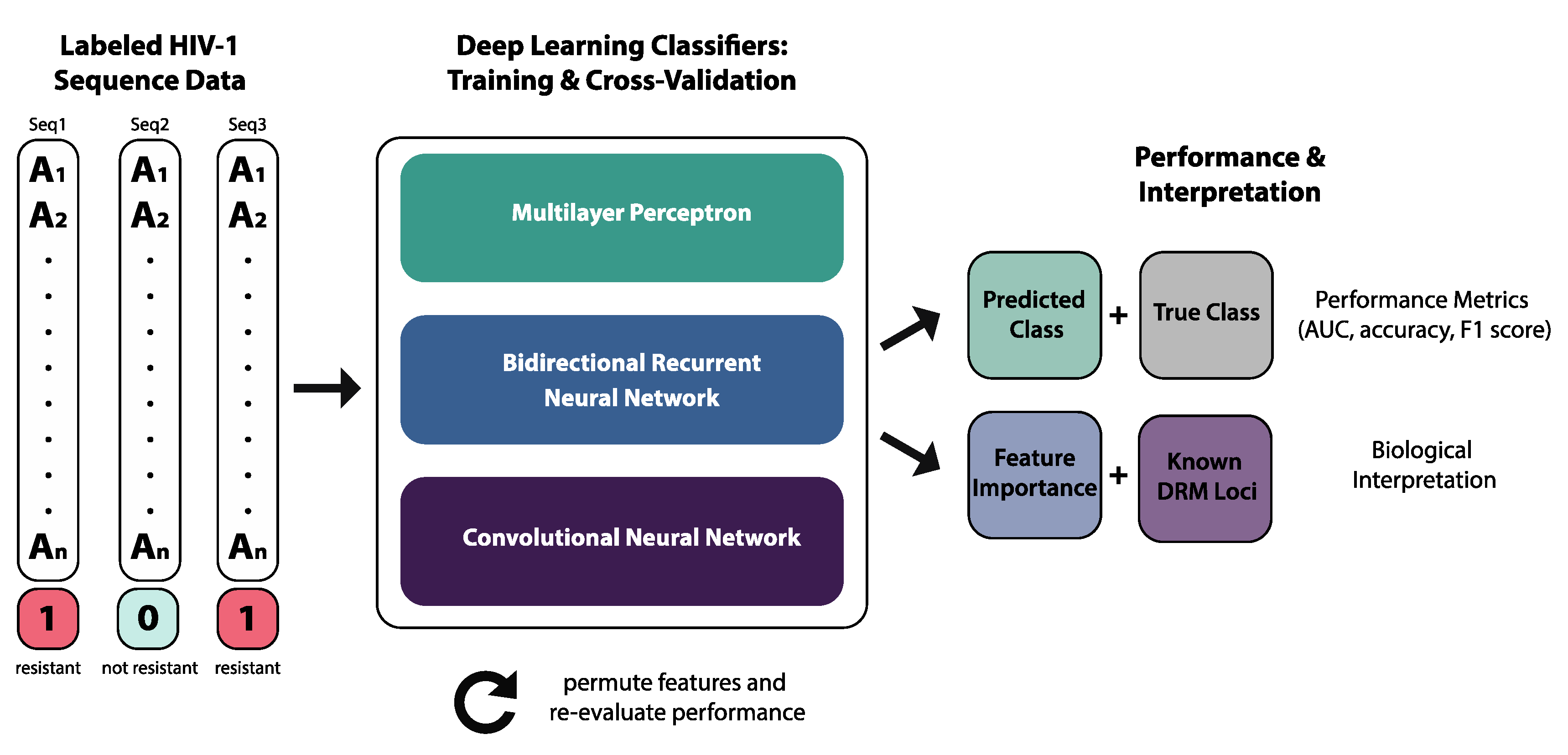
2.2. Deep Learning Classifiers
2.2.1. Multilayer Perceptron
2.2.2. Bidirectional Recurrent Neural Network
2.2.3. Convolutional Neural Network
2.3. Performance Metrics
2.4. Model Interpretation
2.5. Phylogenetics
3. Results
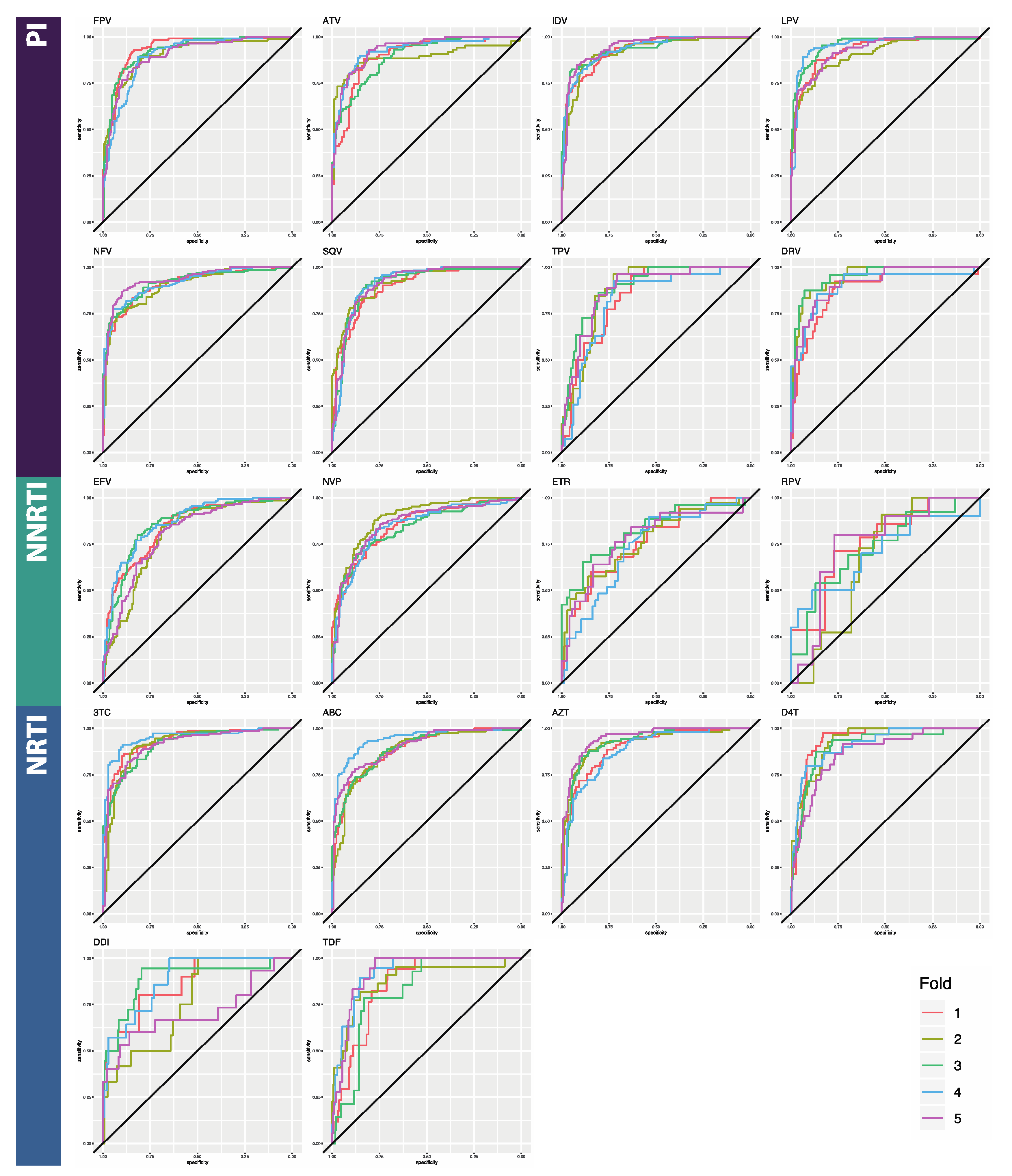
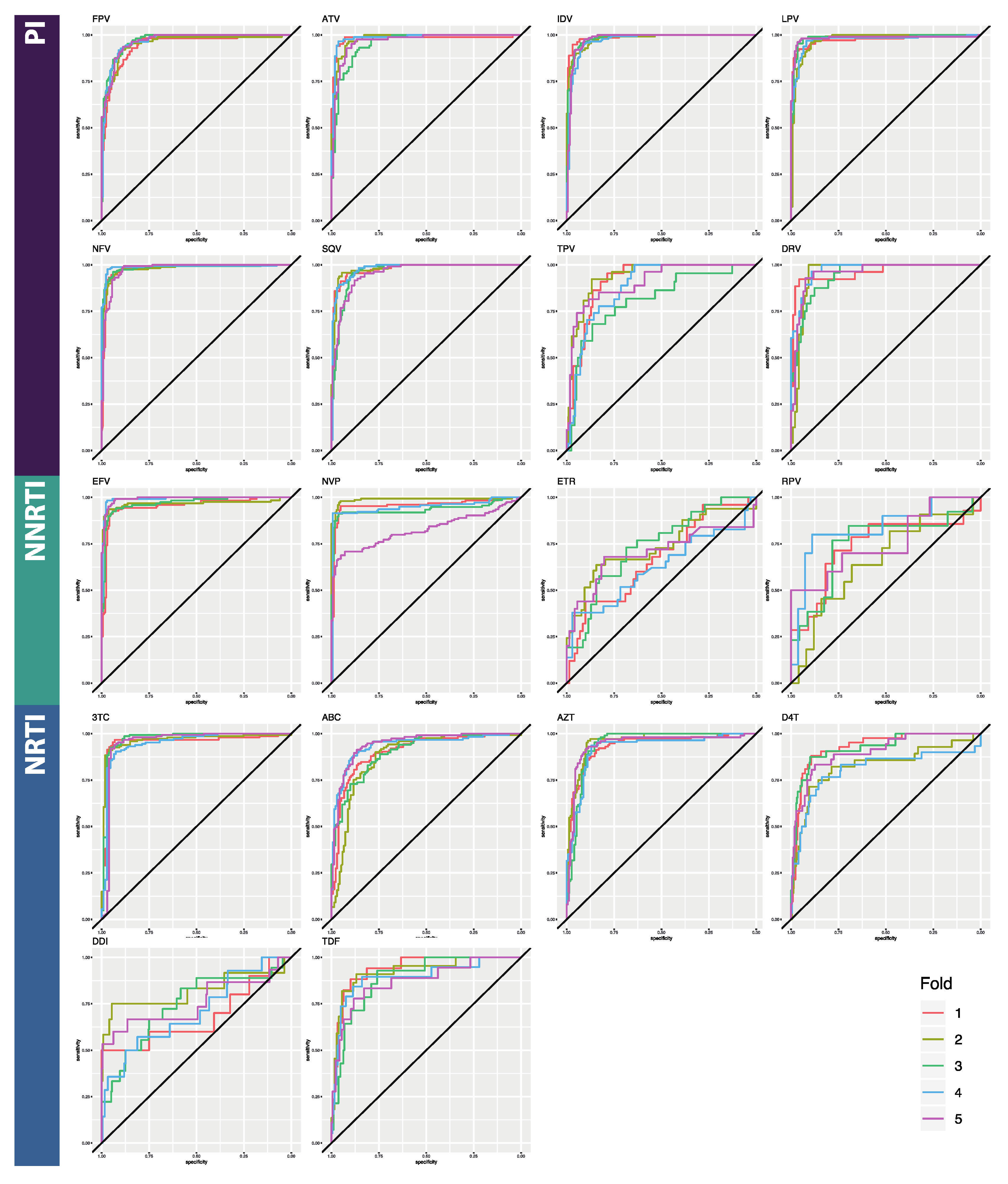
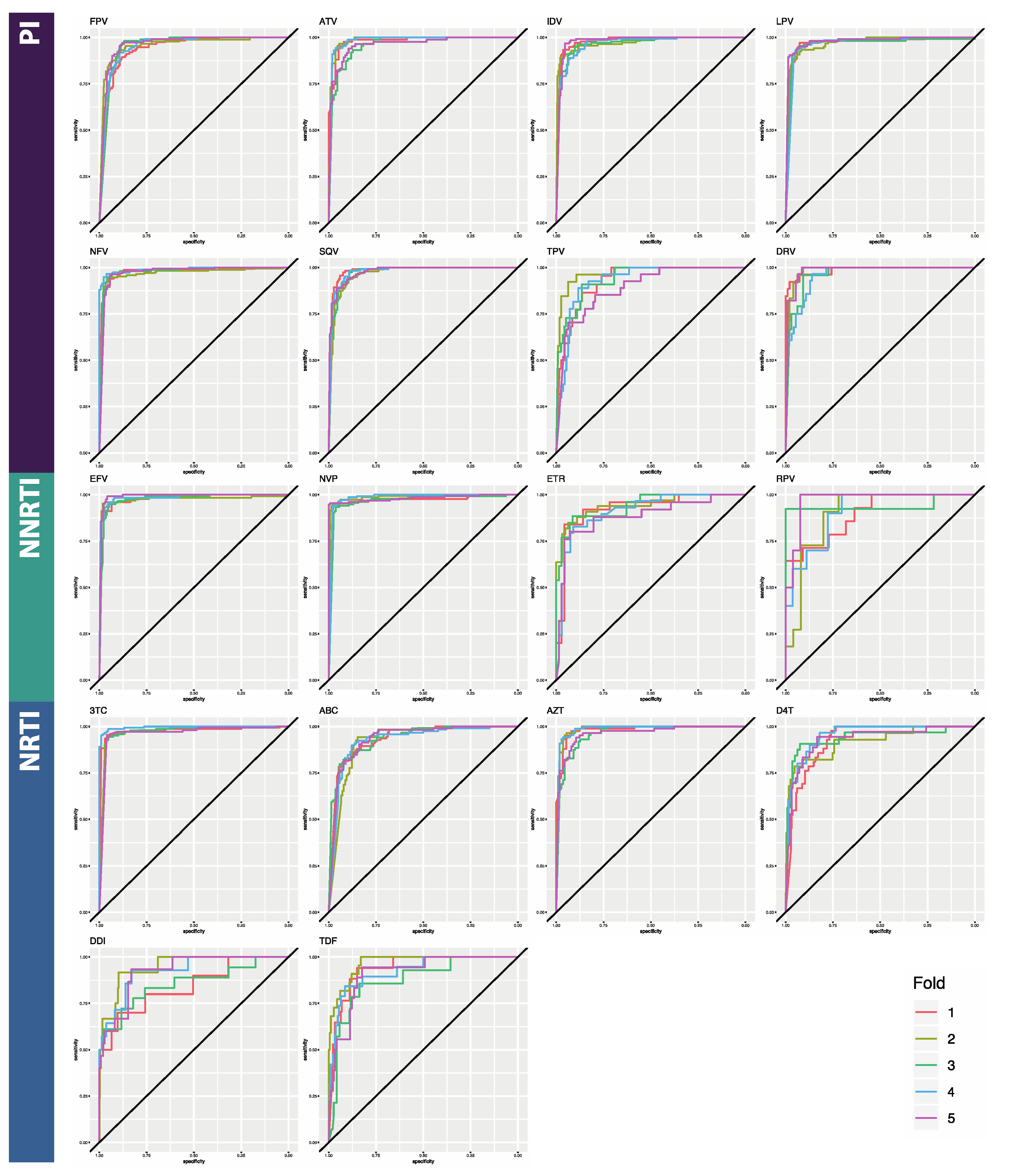
3.1. Classifier Performance
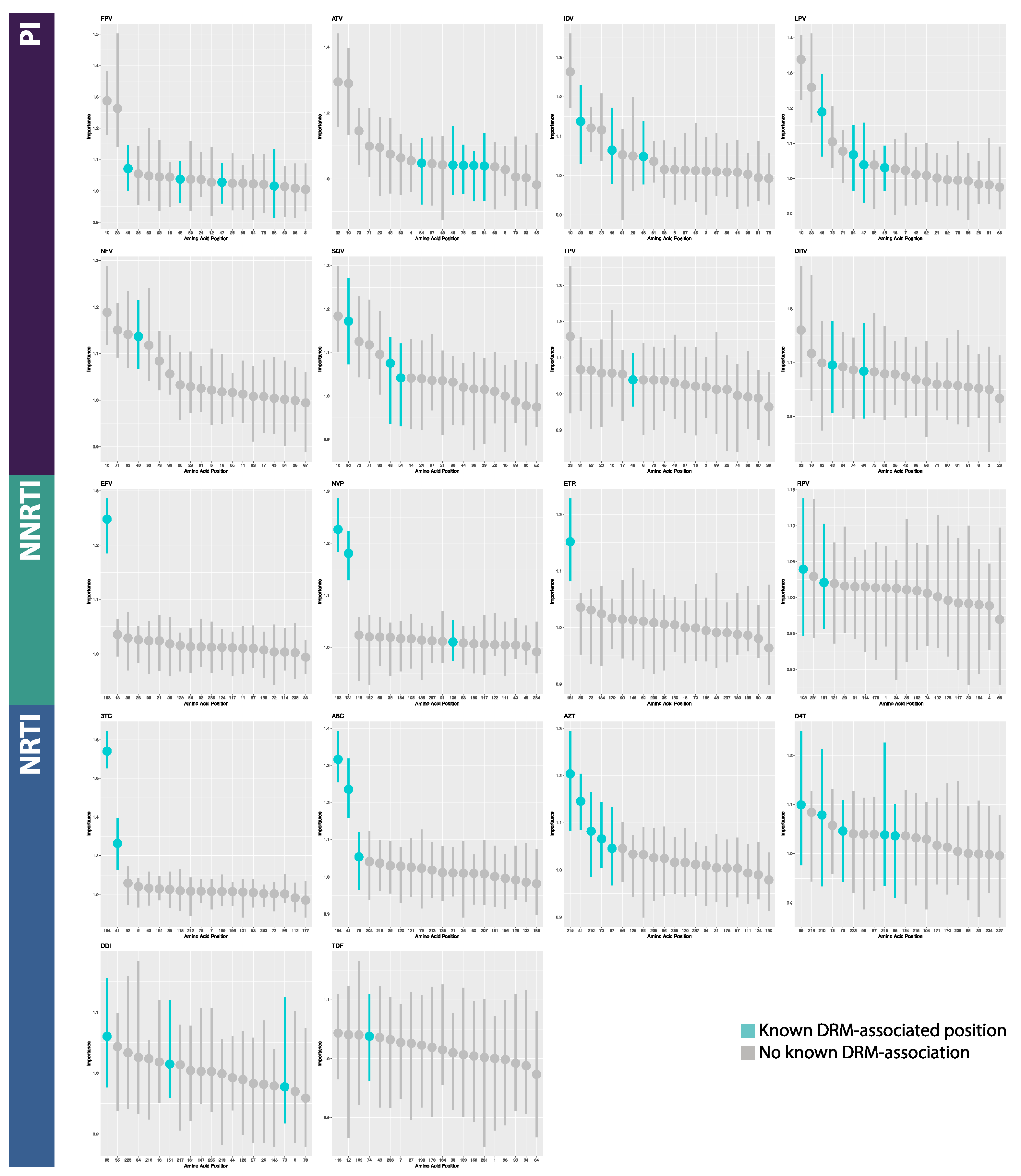
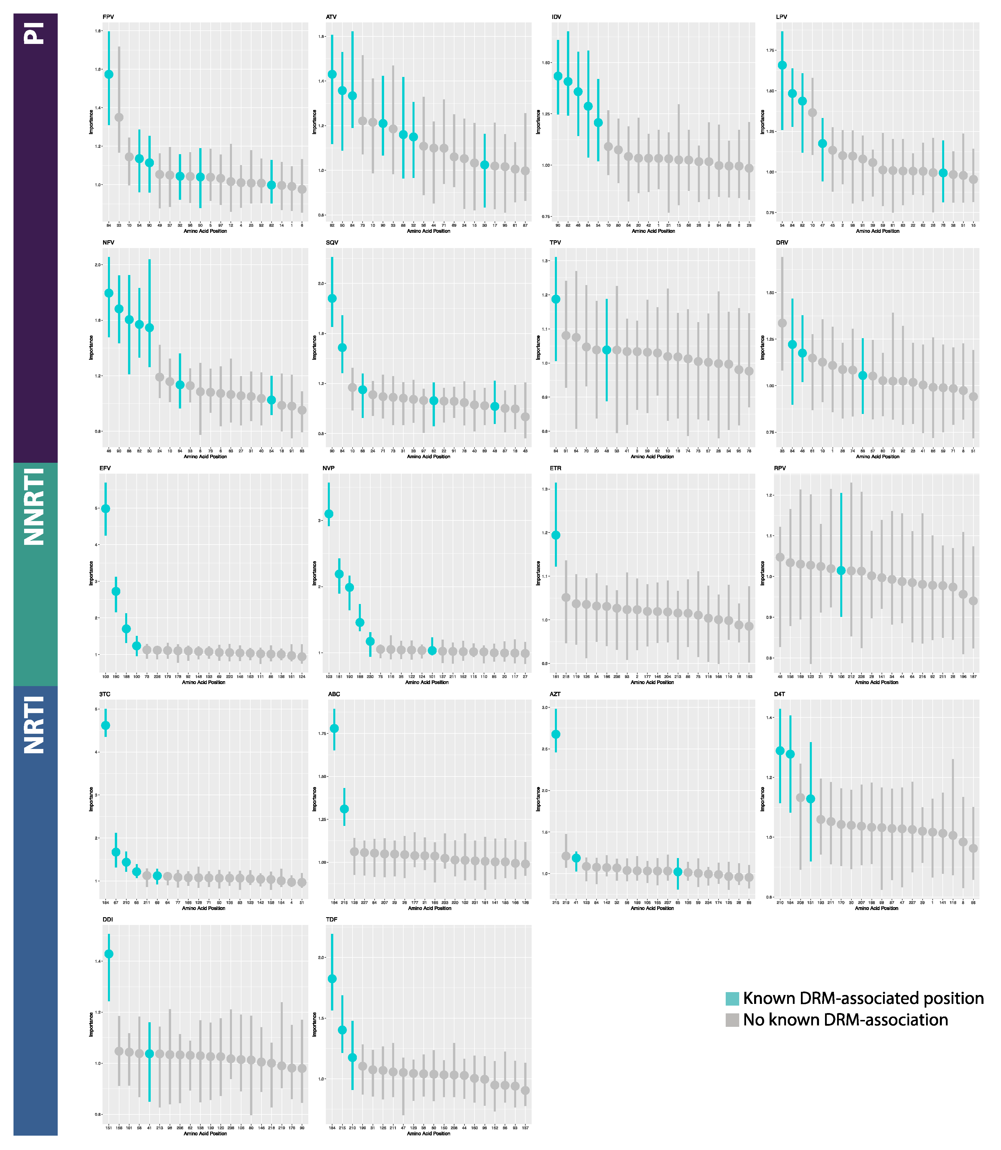
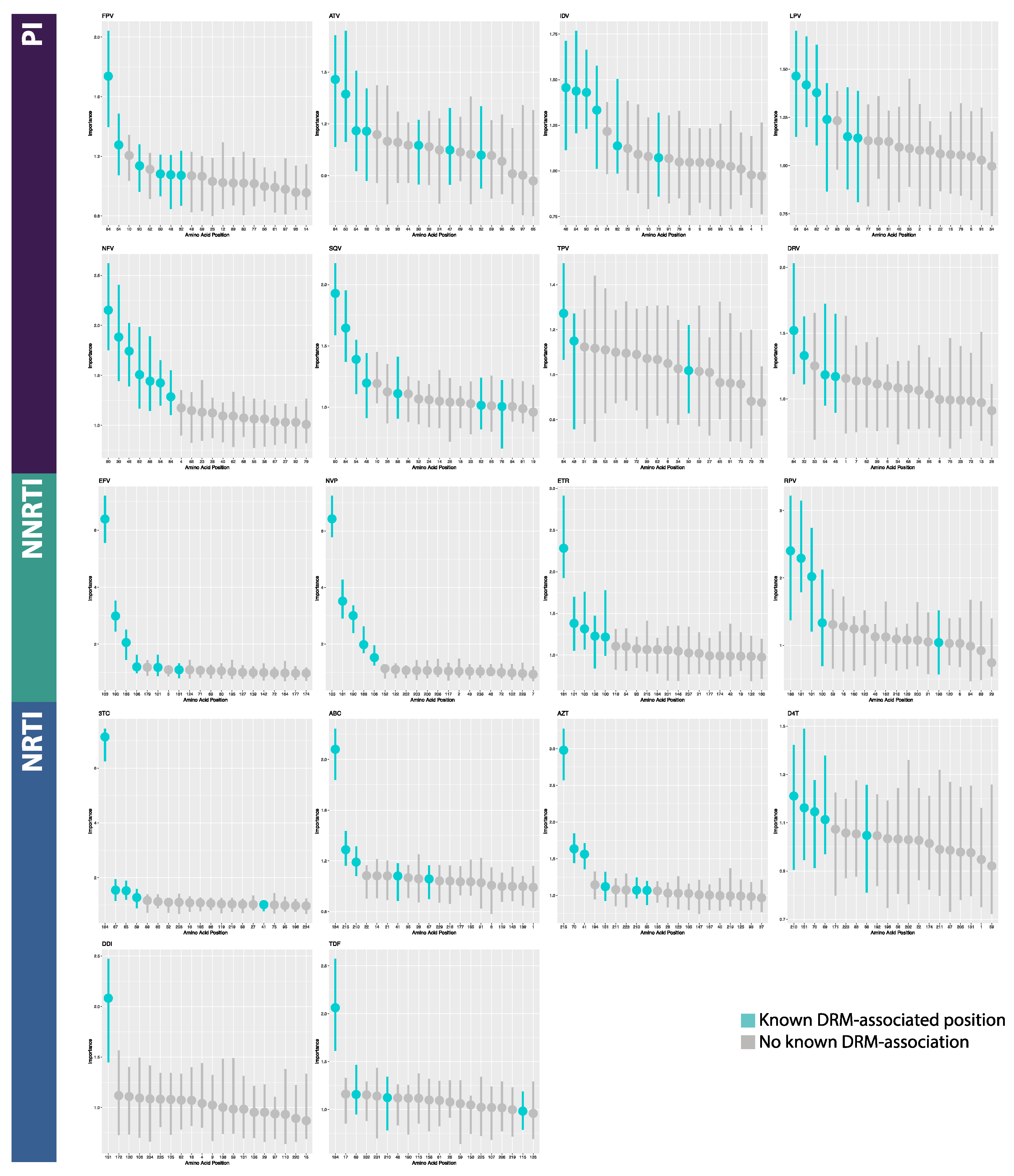
3.2. Model Interpretation
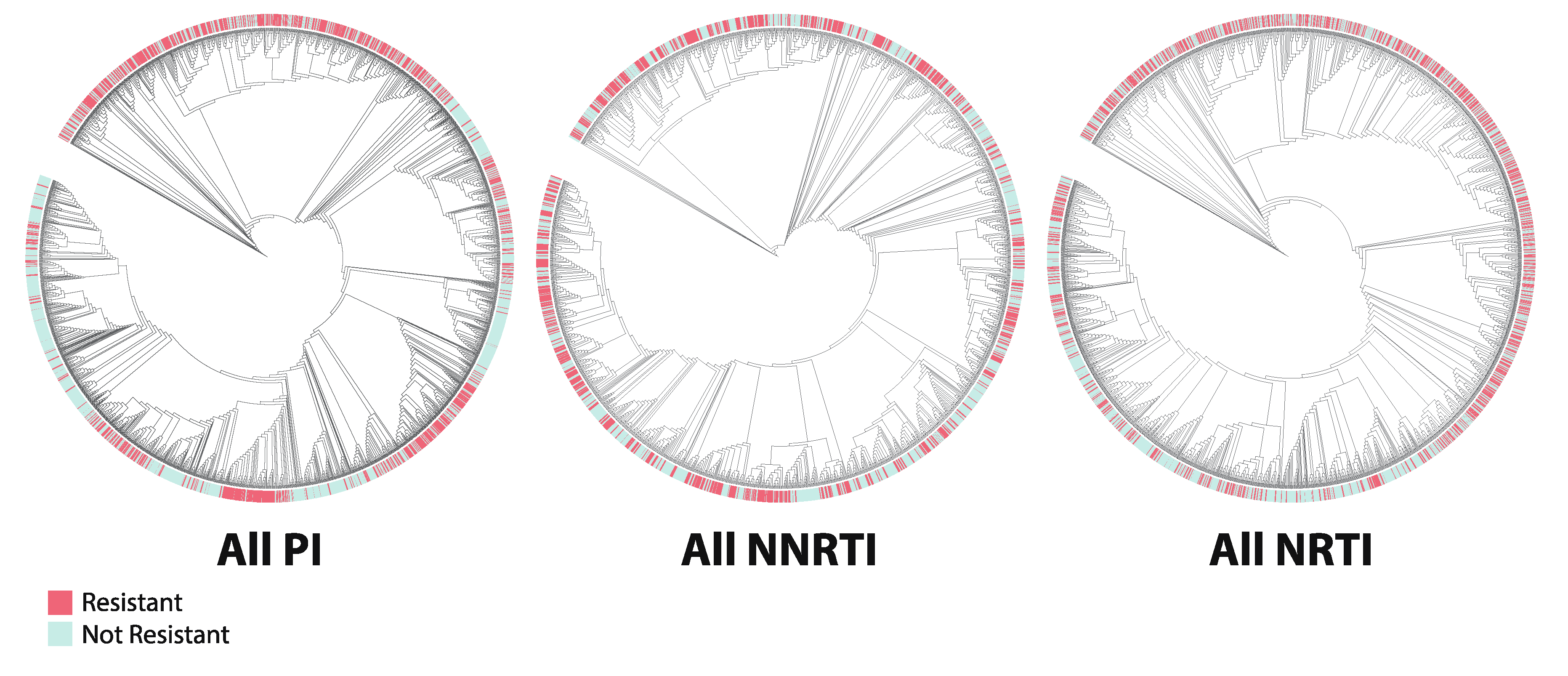
3.3. Phylogenetics
4. Discussion
4.1. Model Performance
4.2. Model Interpretation
4.3. Phylogenetics
4.4. Limitations
4.5. Future Work: Further Applications of Interpretable Deep Learning in HIV
4.5.1. Intra-Patient and Temporal Data
4.5.2. Multi-Omics Approaches
4.5.3. Applications to Other Viruses
5. Conclusions
Supplementary Materials
Author Contributions
Acknowledgments
Conflicts of Interest
Abbreviations
Appendix A
| MLP | |||||||
|---|---|---|---|---|---|---|---|
| Class | Drug | Accuracy | Loss | TPR | TNR | FPR | FNR |
| PI | FPV | 0.839 [0.029] | 0.391 [0.064] | 0.738 [0.114] | 0.895 [0.029] | 0.105 [0.029] | 0.262 [0.114] |
| PI | ATV | 0.830 [0.026] | 0.400 [0.038] | 0.862 [0.061] | 0.805 [0.075] | 0.195 [0.075] | 0.138 [0.061] |
| PI | IDV | 0.858 [0.016] | 0.360 [0.030] | 0.800 [0.063] | 0.908 [0.042] | 0.092 [0.042] | 0.200 [0.063] |
| PI | LPV | 0.852 [0.042] | 0.347 [0.055] | 0.826 [0.060] | 0.868 [0.075] | 0.132 [0.075] | 0.174 [0.060] |
| PI | NFV | 0.819 [0.020] | 0.408 [0.040] | 0.839 [0.081] | 0.799 [0.118] | 0.201 [0.118] | 0.161 [0.081] |
| PI | SQV | 0.843 [0.015] | 0.414 [0.030] | 0.850 [0.101] | 0.826 [0.061] | 0.174 [0.061] | 0.150 [0.101] |
| PI | TPV | 0.734 [0.076] | 0.539 [0.111] | 0.812 [0.169] | 0.720 [0.119] | 0.280 [0.119] | 0.188 [0.169] |
| PI | DRV | 0.835 [0.049] | 0.391 [0.073] | 0.780 [0.173] | 0.851 [0.093] | 0.149 [0.093] | 0.220 [0.173] |
| PI AVERAGE | 0.826 [0.039] | 0.406 [0.058] | 0.813 [0.041] | 0.834 [0.061] | 0.166 [0.061] | 0.187 [0.041] | |
| NNRTI | EFV | 0.709 [0.044] | 0.584 [0.060] | 0.753 [0.194] | 0.683 [0.198] | 0.317 [0.198] | 0.247 [0.194] |
| NNRTI | NVP | 0.767 [0.033] | 0.510 [0.036] | 0.816 [0.089] | 0.725 [0.108] | 0.275 [0.108] | 0.184 [0.089] |
| NNRTI | ETR | 0.659 [0.145] | 0.622 [0.164] | 0.524 [0.378] | 0.721 [0.318] | 0.279 [0.318] | 0.476 [0.378] |
| NNRTI | RPV | 0.690 [0.079] | 0.627 [0.044] | 0.554 [0.210] | 0.741 [0.149] | 0.259 [0.149] | 0.446 [0.210] |
| NNRTI AVERAGE | 0.706 [0.095] | 0.586 [0.143] | 0.662 [0.140] | 0.718 [0.105] | 0.282 [0.105] | 0.338 [0.140] | |
| NRTI | 3TC | 0.839 [0.030] | 0.368 [0.047] | 0.859 [0.072] | 0.811 [0.095] | 0.189 [0.095] | 0.141 [0.072] |
| NRTI | ABC | 0.811 [0.026] | 0.455 [0.061] | 0.742 [0.076] | 0.866 [0.107] | 0.134 [0.107] | 0.258 [0.076] |
| NRTI | AZT | 0.711 [0.173] | 0.769 [0.605] | 0.717 [0.250] | 0.716 [0.415] | 0.284 [0.415] | 0.283 [0.250] |
| NRTI | D4T | 0.867 [0.032] | 0.308 [0.078] | 0.704 [0.097] | 0.891 [0.046] | 0.109 [0.046] | 0.296 [0.097] |
| NRTI | DDI | 0.709 [0.256] | 0.572 [0.518] | 0.613 [0.301] | 0.714 [0.283] | 0.286 [0.283] | 0.387 [0.301] |
| NRTI | TDF | 0.831 [0.047] | 0.344 [0.069] | 0.717 [0.164] | 0.842 [0.061] | 0.158 [0.061] | 0.283 [0.164] |
| NRTI AVERAGE | 0.795 [0.061] | 0.470 [0.150] | 0.725 [0.112] | 0.807 [0.081] | 0.193 [0.081] | 0.275 [0.112] | |
| BRNN | |||||||
|---|---|---|---|---|---|---|---|
| Class | Drug | Accuracy | Loss | TPR | TNR | FPR | FNR |
| PI | FPV | 0.898 [0.012] | 0.298 [0.050] | 0.900 [0.024] | 0.898 [0.014] | 0.102 [0.014] | 0.100 [0.024] |
| PI | ATV | 0.925 [0.026] | 0.259 [0.102] | 0.930 [0.027] | 0.921 [0.045] | 0.079 [0.045] | 0.070 [0.027] |
| PI | IDV | 0.935 [0.011] | 0.225 [0.050] | 0.926 [0.025] | 0.940 [0.029] | 0.060 [0.029] | 0.074 [0.025] |
| PI | LPV | 0.936 [0.023] | 0.219 [0.059] | 0.919 [0.042] | 0.949 [0.020] | 0.051 [0.020] | 0.081 [0.042] |
| PI | NFV | 0.941 [0.014] | 0.208 [0.050] | 0.938 [0.017] | 0.945 [0.024] | 0.055 [0.024] | 0.062 [0.017] |
| PI | SQV | 0.918 [0.023] | 0.292 [0.091] | 0.913 [0.022] | 0.922 [0.029] | 0.078 [0.029] | 0.087 [0.022] |
| PI | TPV | 0.845 [0.021] | 0.469 [0.130] | 0.745 [0.065] | 0.865 [0.021] | 0.135 [0.021] | 0.255 [0.065] |
| PI | DRV | 0.896 [0.044] | 0.349 [0.176] | 0.851 [0.098] | 0.910 [0.070] | 0.090 [0.070] | 0.149 [0.098] |
| PI AVERAGE | 0.912 [0.032] | 0.290 [0.087] | 0.890 [0.065] | 0.919 [0.028] | 0.081 [0.028] | 0.110 [0.065] | |
| NNRTI | EFV | 0.946 [0.018] | 0.188 [0.055] | 0.925 [0.023] | 0.961 [0.022] | 0.039 [0.022] | 0.075 [0.023] |
| NNRTI | NVP | 0.917 [0.063] | 0.261 [0.122] | 0.881 [0.102] | 0.952 [0.027] | 0.048 [0.027] | 0.119 [0.102] |
| NNRTI | ETR | 0.946 [0.018] | 0.188 [0.055] | 0.925 [0.023] | 0.961 [0.022] | 0.039 [0.022] | 0.075 [0.023] |
| NNRTI | RPV | 0.729 [0.033] | 0.701 [0.192] | 0.583 [0.189] | 0.783 [0.102] | 0.217 [0.102] | 0.417 [0.189] |
| NNRTI AVERAGE | 0.884 [0.104] | 0.334 [0.247] | 0.829 [0.165] | 0.914 [0.088] | 0.086 [0.088] | 0.171 [0.165] | |
| NRTI | 3TC | 0.931 [0.013] | 0.247 [0.044] | 0.938 [0.027] | 0.923 [0.023] | 0.077 [0.023] | 0.062 [0.027] |
| NRTI | ABC | 0.842 [0.029] | 0.505 [0.139] | 0.819 [0.025] | 0.862 [0.039] | 0.138 [0.039] | 0.181 [0.025] |
| NRTI | AZT | 0.890 [0.011] | 0.407 [0.087] | 0.891 [0.037] | 0.887 [0.032] | 0.113 [0.032] | 0.109 [0.037] |
| NRTI | D4T | 0.892 [0.017] | 0.333 [0.041] | 0.705 [0.060] | 0.919 [0.018] | 0.081 [0.018] | 0.295 [0.060] |
| NRTI | DDI | 0.909 [0.025] | 0.278 [0.064] | 0.478 [0.137] | 0.935 [0.020] | 0.065 [0.020] | 0.522 [0.137] |
| NRTI | TDF | 0.911 [0.023] | 0.374 [0.085] | 0.673 [0.178] | 0.934 [0.036] | 0.066 [0.036] | 0.327 [0.178] |
| NRTI AVERAGE | 0.896 [0.030] | 0.357 [0.094] | 0.751 [0.168] | 0.910 [0.029] | 0.090 [0.029] | 0.249 [0.168] | |
| CNN | |||||||
|---|---|---|---|---|---|---|---|
| Class | Drug | Accuracy | Loss | TPR | TNR | FPR | FNR |
| PI | FPV | 0.901 [0.017] | 0.980 [0.252] | 0.879 [0.053] | 0.913 [0.027] | 0.087 [0.027] | 0.121 [0.053] |
| PI | ATV | 0.922 [0.029] | 0.610 [0.195] | 0.908 [0.043] | 0.932 [0.048] | 0.068 [0.048] | 0.092 [0.043] |
| PI | IDV | 0.932 [0.018] | 0.622 [0.134] | 0.914 [0.028] | 0.945 [0.021] | 0.055 [0.021] | 0.086 [0.028] |
| PI | LPV | 0.946 [0.007] | 0.542 [0.166] | 0.942 [0.015] | 0.951 [0.015] | 0.049 [0.015] | 0.058 [0.015] |
| PI | NFV | 0.920 [0.008] | 0.671 [0.114] | 0.880 [0.012] | 0.944 [0.013] | 0.056 [0.013] | 0.120 [0.012] |
| PI | SQV | 0.920 [0.013] | 0.671 [0.090] | 0.880 [0.038] | 0.944 [0.008] | 0.0562 [0.008] | 0.120 [0.038] |
| PI | TPV | 0.884 [0.031] | 1.133 [0.339] | 0.680 [0.106] | 0.929 [0.033] | 0.071 [0.033] | 0.320 [0.106] |
| PI | DRV | 0.927 [0.026] | 0.733 [0.353] | 0.834 [0.085] | 0.954 [0.029] | 0.046 [0.029] | 0.166 [0.085] |
| PI AVERAGE | 0.919 [0.019] | 0.745 [0.204] | 0.865 [0.081] | 0.939 [0.013] | 0.061 [0.013] | 0.135 [0.081] | |
| NNRTI | EFV | 0.951 [0.010] | 0.398 [0.107] | 0.926 [0.020] | 0.969 [0.008] | 0.0313 [0.008] | 0.074 [0.020] |
| NNRTI | NVP | 0.954 [0.011] | 0.455 [0.076] | 0.933 [0.038] | 0.971 [0.024] | 0.029 [0.024] | 0.067 [0.038] |
| NNRTI | ETR | 0.878 [0.022] | 0.777 [0.339] | 0.783 [0.056] | 0.916 [0.025] | 0.084 [0.025] | 0.217 [0.059] |
| NNRTI | RPV | 0.862 [0.076] | 0.826 [0.409] | 0.739 [0.108] | 0.924 [0.091] | 0.076 [0.091] | 0.261 [0.108] |
| NNRTI AVERAGE | 0.911 [0.048] | 0.614 [0.219] | 0.845 [0.099] | 0.945 [0.029] | 0.055 [0.029] | 0.155 [0.099] | |
| NRTI | 3TC | 0.946 [0.012] | 0.591 [0.183] | 0.945 [0.011] | 0.948 [0.030] | 0.052 [0.030] | 0.055 [0.011] |
| NRTI | ABC | 0.862 [0.007] | 1.283 [0.143] | 0.847 [0.018] | 0.874 [0.012] | 0.126 [0.012] | 0.153 [0.018] |
| NRTI | AZT | 0.901 [0.019] | 0.874 [0.278] | 0.884 [0.057] | 0.913 [0.020] | 0.087 [0.020] | 0.116 [0.057] |
| NRTI | D4T | 0.922 [0.025] | 0.785 [0.310] | 0.722 [0.071] | 0.952 [0.021] | 0.048 [0.021] | 0.278 [0.071] |
| NRTI | DDI | 0.959 [0.008] | 0.482 [0.073] | 0.497 [0.065] | 0.985 [0.014] | 0.015 [0.014] | 0.503 [0.065] |
| NRTI | TDF | 0.933 [0.016] | 0.813 [0.168] | 0.561 [0.096] | 0.968 [0.013] | 0.032 [0.013] | 0.439 [0.096] |
| NRTI AVERAGE | 0.920 [0.035] | 0.805 [0.277] | 0.743 [0.182] | 0.940 [0.040] | 0.060 [0.040] | 0.257 [0.182] | |
| Model | MLP | BRNN | CNN | |||
|---|---|---|---|---|---|---|
| AUC | F1 | AUC | F1 | AUC | F1 | |
| ATV | 0.899 [0.019] | 0.765 [0.062] | 0.980 [0.013] | 0.865 [0.018] | 0.981 [0.012] | 0.866 [0.019] |
| DRV | 0.872 [0.032] | 0.815 [0.021] | 0.960 [0.011] | 0.915 [0.027] | 0.987 [0.013] | 0.910 [0.033] |
| FPV | 0.934 [0.016] | 0.830 [0.019] | 0.945 [0.011] | 0.925 [0.016] | 0.937 [0.009] | 0.922 [0.015] |
| IDV | 0.928 [0.009] | 0.831 [0.048] | 0.988 [0.006] | 0.928 [0.024] | 0.979 [0.007] | 0.925 [0.008] |
| LPV | 0.926 [0.021] | 0.829 [0.019] | 0.975 [0.006] | 0.944 [0.014] | 0.973 [0.006] | 0.948 [0.010] |
| NFV | 0.906 [0.012] | 0.809 [0.043] | 0.979 [0.004] | 0.894 [0.027] | 0.976 [0.009] | 0.891 [0.025] |
| SQV | 0.897 [0.008] | 0.523 [0.064] | 0.976 [0.011] | 0.630 [0.065] | 0.981 [0.005] | 0.673 [0.091] |
| TPV | 0.842 [0.029] | 0.669 [0.067] | 0.916 [0.049] | 0.782 [0.077] | 0.93 [0.028] | 0.831 [0.060] |
| PI AVERAGE | 0.9 [0.009] | 0.732 [0.135] | 0.965 [0.014] | 0.860 [0.106] | 0.968 [0.007] | 0.871 [0.088] |
| EFV | 0.843 [0.033] | 0.676 [0.043] | 0.953 [0.017] | 0.934 [0.021] | 0.980 [0.007] | 0.940 [0.013] |
| ETR | 0.764 [0.032] | 0.768 [0.034] | 0.669 [0.049] | 0.910 [0.067] | 0.926 [0.023] | 0.950 [0.016] |
| NVP | 0.853 [0.022] | 0.415 [0.209] | 0.957 [0.062] | 0.934 [0.021] | 0.976 [0.008] | 0.783 [0.044] |
| RPV | 0.760 [0.037] | 0.524 [0.139] | 0.740 [0.062] | 0.567 [0.102] | 0.896 [0.032] | 0.770 [0.126] |
| NNRTI AVERAGE | 0.805 [0.006] | 0.596 [0.157] | 0.830 [0.021] | 0.836 [0.180] | 0.945 [0.012] | 0.861 [0.097] |
| ABC | 0.887 [0.025] | 0.861 [0.031] | 0.904 [0.026] | 0.941 [0.103] | 0.935 [0.007] | 0.953 [0.010] |
| AZT | 0.901 [0.025] | 0.783 [0.017] | 0.934 [0.012] | 0.828 [0.028] | 0.944 [0.012] | 0.849 [0.009] |
| DDI | 0.861 [0.081] | 0.681 [0.100] | 0.682 [0.053] | 0.871 [0.009] | 0.842 [0.047] | 0.881 [0.027] |
| DFT | 0.935 [0.025] | 0.579 [0.050] | 0.928 [0.057] | 0.625 [0.083] | 0.926 [0.013] | 0.709 [0.051] |
| TDF | 0.853 [0.044] | 0.224 [0.107] | 0.939 [0.027] | 0.362 [0.116] | 0.940 [0.034] | 0.559 [0.095] |
| TTC | 0.933 [0.017] | 0.430 [0.096] | 0.952 [0.010] | 0.564 [0.100] | 0.977 [0.013] | 0.589 [0.119] |
| NRTI AVERAGE | 0.895 [0.024] | 0.593 [0.236] | 0.89 [0.020] | 0.698 [0.220] | 0.927 [0.016] | 0.757 [0.163] |
References
- Centers for Disease Control and Prevention. HIV Surveillance Report; Centers for Disease Control and Prevention: Atlanta, GA, USA, 2018; Volume 30. [Google Scholar]
- Wandeler, G.; Johnson, L.F.; Egger, M. Trends in life expectancy of HIV-positive adults on ART across the globe: Comparisons with general population HHS Public Access. Curr. Opin. HIV AIDS 2016, 11, 492–500. [Google Scholar] [CrossRef] [PubMed]
- Das, M.; Chu, P.L.; Santos, G.M.; Scheer, S.; Vittinghoff, E.; McFarland, W.; Colfax, G.N. Decreases in community viral load are accompanied by reductions in new HIV infections in San Francisco. PLoS ONE 2010, 5, e11068. [Google Scholar] [CrossRef]
- Quinn, T.C.; Wawer, M.J.; Sewankambo, N.; Serwadda, D.; Li, C.; Wabwire-Mangen, F.; Meehan, M.O.; Lutalo, T.; Gray, R.H. Viral load and heterosexual transmission of human immunodeficiency virus type 1. N. Engl. J. Med. 2000, 342, 921–929. [Google Scholar] [CrossRef] [PubMed]
- Rambaut, A.; Posada, D.; Crandall, K.A.; Holmes, E.C. The causes and consequences of HIV evolution. Nat. Rev. Genet. 2004, 5, 52–61. [Google Scholar] [CrossRef] [PubMed]
- Crandall, K.A.; Kelsey, C.R.; Imamichi, H.; Lane, H.C.; Salzman, N.P. Parallel evolution of drug resistance in HIV: Failure of nonsynonymous/synonymous substitution rate ratio to detect selection. Mol. Biol. Evol. 1999, 16, 372–382. [Google Scholar] [CrossRef] [PubMed]
- Hirsch, M.S.; Conway, B.; D’Aquila, R.T.; Johnson, V.A.; Brun-Vézinet, F.; Clotet, B.; Demeter, L.M.; Hammer, S.M.; Jacobsen, D.M.; Kuritzkes, D.R.; et al. Antiretroviral drug resistance testing in adults with HIV infection: Implications for clinical management. J. Am. Med. Assoc. 1998, 279, 1984–1991. [Google Scholar] [CrossRef] [PubMed]
- Zhang, J.; Rhee, S.Y.; Taylor, J.; Shafer, R.W. Comparison of the precision and sensitivity of the antivirogram and PhenoSense HIV drug susceptibility assays. J. Acquir. Immune Defic. Syndr. 2005, 38, 439–444. [Google Scholar] [CrossRef]
- Rhee, S.Y.; Gonzales, M.J.; Kantor, R.; Betts, B.J.; Ravela, J.; Shafer, R.W. Human immunodeficiency virus reverse transcriptase and protease sequence database. Nucleic Acids Res. 2003, 31, 298–303. [Google Scholar] [CrossRef]
- Bonet, I.; García, M.M.; Saeys, Y.; Van De Peer, Y.; Grau, R. Predicting human immunodeficiency virus (HIV) drug resistance using recurrent neural networks. In Proceedings of the IWINAC 2007, La Manga del Mar Menor, Spain, 18–21 June 2007; Volume 4527, pp. 234–243. [Google Scholar]
- Liu, T.; Shafer, R. Web Resources for HIV type 1 Genotypic-Resistance Test Interpretation. Clin. Infect. Dis. 2006, 42, 1608–1618. [Google Scholar] [CrossRef]
- Jensen, M.A.; Coetzer, M.; van ’t Wout, A.B.; Morris, L.; Mullins, J.I. A Reliable Phenotype Predictor for Human Immunodeficiency Virus Type 1 Subtype C Based on Envelope V3 Sequences. J. Virol. 2006, 80, 4698–4704. [Google Scholar] [CrossRef]
- Beerenwinkel, N.; Däumer, M.; Oette, M.; Korn, K.; Hoffmann, D.; Kaiser, R.; Lengauer, T.; Selbig, J.; Walter, H. Geno2pheno: Estimating phenotypic drug resistance from HIV-1 genotypes. Nucleic Acids Res. 2003, 31, 3850–3855. [Google Scholar] [CrossRef]
- Riemenschneider, M.; Hummel, T.; Heider, D. SHIVA—A web application for drug resistance and tropism testing in HIV. BMC Bioinform. 2016, 17, 314. [Google Scholar] [CrossRef] [PubMed]
- Riemenschneider, M.; Cashin, K.Y.; Budeus, B.; Sierra, S.; Shirvani-Dastgerdi, E.; Bayanolhagh, S.; Kaiser, R.; Gorry, P.R.; Heider, D. Genotypic Prediction of Co-receptor Tropism of HIV-1 Subtypes A and C. Sci. Rep. 2016, 6, 1–9. [Google Scholar] [CrossRef] [PubMed]
- Heider, D.; Senge, R.; Cheng, W.; Hüllermeier, E. Multilabel classification for exploiting cross-resistance information in HIV-1 drug resistance prediction. Bioinformatics 2013, 29, 1946–1952. [Google Scholar] [CrossRef] [PubMed]
- Beerenwinkel, N.; Schmidt, B.; Walter, H.; Kaiser, R.; Lengauer, T.; Hoffmann, D.; Korn, K.; Selbig, J. Diversity and complexity of HIV-1 drug resistance: A bioinformatics approach to predicting phenotype from genotype. Proc. Natl. Acad. Sci. USA 2002, 99, 8271–8276. [Google Scholar] [CrossRef]
- Wang, D.; Larder, B. Networks Enhanced Prediction of Lopinavir Resistance from Genotype by Use of Artificial Neural Networks. J. Infect. Dis. 2003, 188, 653–660. [Google Scholar] [CrossRef]
- Sheik Amamuddy, O.; Bishop, N.T.; Tastan Bishop, Ö. Improving fold resistance prediction of HIV-1 against protease and reverse transcriptase inhibitors using artificial neural networks. BMC Bioinform. 2017, 18, 369. [Google Scholar] [CrossRef]
- Ekpenyong, M.E.; Etebong, P.I.; Jackson, T.C. Fuzzy-multidimensional deep learning for efficient prediction of patient response to antiretroviral therapy. Heliyon 2019, 5, e02080. [Google Scholar] [CrossRef]
- Angermueller, C.; Pärnamaa, T.; Parts, L.; Stegle, O. Deep learning for computational biology. Mol. Syst. Biol. 2016, 12, 878. [Google Scholar] [CrossRef]
- Min, S.; Lee, B.; Yoon, S. Deep learning in bioinformatics. Brief. Bioinform. 2017, 18, 851–869. [Google Scholar] [CrossRef]
- Molnar, C. iml: An R package for Interpretable Machine Learning. J. Open Source Softw. 2018, 3, 786. [Google Scholar] [CrossRef]
- R Core Team. R: A Language and Environment for Statistical Computing; R Foundation for Statistical Computing: Vienna, Austria, 2017. [Google Scholar]
- RStudio Team. RStudio: Integrated Development Environment for R; R Studio, Inc.: Boston, MA, USA, 2015. [Google Scholar]
- Chollet, F.; Allaire, J.J. Keras: R Interface to Keras; Keras Team. 2017. Available online: https://keras.rstudio.com/index.html (accessed on 21 April 2020).
- Abadi, M.; Agarwal, A.; Barham, P.; Brevdo, E.; Chen, Z.; Citro, C.; Corrado, G.S.; Davis, A.; Dean, J.; Devin, M.; et al. TensorFlow: Large-Scale Machine Learning on Heterogeneous Systems [White Paper]; Google Research: Palo Alto, CA, USA, 2015. [Google Scholar]
- Van Rossum, G.; Drake, F.L. Python 3 Reference Manual; CreateSpace: Scotts Valley, CA, USA, 2009; ISBN 1441412697. [Google Scholar]
- Wickham, H. ggplot2: Elegant Graphics for Data Analysis; Springer: New York, NY, USA, 2016; ISBN 978-3-319-24277-4. [Google Scholar]
- Robin, X.; Turck, N.; Hainard, A.; Tiberti, N.; Lisacek, F.; Sanchez, J.-C.; Müller, M. pROC: An open-source package for R and S+ to analyze and compare ROC curves. BMC Bioinform. 2011, 12, 77. [Google Scholar] [CrossRef] [PubMed]
- Fisher, A.; Rudin, C.; Dominici, F. All models are wrong, but many are useful: Learning a variable’s importance by studying an entire class of prediction models simultaneously. J. Mach. Learn. Res. 2019, 20, 1–81. [Google Scholar]
- Darriba, D.; Posada, D.; Kozlov, A.M.; Stamatakis, A.; Morel, B.; Flouri, T. ModelTest-NG: A New and Scalable Tool for the Selection of DNA and Protein Evolutionary Models. Mol. Biol. Evol. 2019, 37, 291–294. [Google Scholar] [CrossRef] [PubMed]
- Dang, C.C.; Le, Q.S.; Gascuel, O.; Le, V.S. FLU, an amino acid substitution model for influenza proteins. BMC Evol. Biol. 2010, 10, 99. [Google Scholar] [CrossRef] [PubMed]
- Stamatakis, A. RAxML version 8: A tool for phylogenetic analysis and post-analysis of large phylogenies. Bioinformatics 2014, 30, 1312–1313. [Google Scholar] [CrossRef]
- Miller, M.A.; Pfeiffer, W.; Schwartz, T. Creating the CIPRES Science Gateway for inference of large phylogenetic trees. In Proceedings of the 2010 Gateway Computing Environments Workshop (GCE), New Orleans, LA, USA, 14 November 2010. [Google Scholar]
- Letunic, I.; Bork, P. Interactive Tree Of Life (iTOL) v4: Recent updates and new developments. Nucleic Acids Res. 2019, 47, W256–W259. [Google Scholar] [CrossRef]
- Shimodaira, H. An approximately unbiased test of phylogenetic tree selection. Syst. Biol. 2002, 51, 492–508. [Google Scholar] [CrossRef]
- Nguyen, L.T.; Schmidt, H.A.; Von Haeseler, A.; Minh, B.Q. IQ-TREE: A fast and effective stochastic algorithm for estimating maximum-likelihood phylogenies. Mol. Biol. Evol. 2015, 32, 268–274. [Google Scholar] [CrossRef]
- Felsenstein, J. Phylogenies and the comparative method. Am. Nat. 1985, 125, 1–15. [Google Scholar] [CrossRef]
- Zanini, F.; Brodin, J.; Thebo, L.; Lanz, C.; Bratt, G.; Albert, J.; Neher, R.A. Population genomics of intrapatient HIV-1 evolution. Elife 2015, 4, e11282. [Google Scholar] [CrossRef] [PubMed]
- Posada-Cespedes, S.; Seifert, D.; Beerenwinkel, N. Recent advances in inferring viral diversity from high-throughput sequencing data. Virus Res. 2017, 239, 17–32. [Google Scholar] [CrossRef] [PubMed]
- Wirden, M.; Malet, I.; Derache, A.; Marcelin, A.G.; Roquebert, B.; Simon, A.; Kirstetter, M.; Joubert, L.M.; Katlama, C.; Calvez, V. Clonal analyses of HIV quasispecies in patients harbouring plasma genotype with K65R mutation associated with thymidine analogue mutations or L74V substitution. AIDS 2005, 19, 630–632. [Google Scholar] [CrossRef]
- Biswas, A.; Haldane, A.; Arnold, E.; Levy, R.M. Epistasis and entrenchment of drug resistance in HIV-1 subtype B. Elife 2019, 8, e50524. [Google Scholar] [CrossRef]
- Castro-Nallar, E.; Pérez-Losada, M.; Burton, G.F.; Crandall, K.A. The evolution of HIV: Inferences using phylogenetics. Mol. Phylogenet. Evol. 2012, 62, 777–792. [Google Scholar] [CrossRef] [PubMed]
- Ching, T.; Himmelstein, D.S.; Beaulieu-Jones, B.K.; Kalinin, A.A.; Do, B.T.; Way, G.P.; Ferrero, E.; Agapow, P.M.; Zietz, M.; Hoffman, M.M.; et al. Opportunities and Obstacles for Deep Learning in Biology and Medicine. J. R. Soc. Interface 2018, 15, 20170387. [Google Scholar] [CrossRef] [PubMed]
- Zou, J.; Huss, M.; Abid, A.; Mohammadi, P.; Torkamani, A.; Telenti, A. A primer on deep learning in genomics. Nat. Genet. 2019, 51, 12–18. [Google Scholar] [CrossRef] [PubMed]
- Margolis, D.M.; Koup, R.A.; Ferrari, G. HIV antibodies for treatment of HIV infection. Immunol. Rev. 2017, 275, 313–323. [Google Scholar] [CrossRef]
- Zitnik, M.; Nguyen, F.; Wang, B.; Leskovec, J.; Goldenberg, A.; Hoffman, M.M. Machine learning for integrating data in biology and medicine: Principles, practice, and opportunities. Inf. Fusion 2019, 50, 71–91. [Google Scholar] [CrossRef]
- Gibson, K.M.; Jair, K.; Castel, A.D.; Bendall, M.L.; Wilbourn, B.; Jordan, J.A.; Crandall, K.A.; Pérez-Losada, M.; Subramanian, T.; Binkley, J.; et al. A cross-sectional study to characterize local HIV-1 dynamics in Washington, DC using next-generation sequencing. Sci. Rep. 2020, 10, 1–18. [Google Scholar] [CrossRef] [PubMed]
- Eliseev, A.; Gibson, K.M.; Avdeyev, P.; Novik, D.; Bendall, M.L.; Pérez-Losada, M.; Alexeev, N.; Crandall, K.A. Evaluation of haplotype callers for next-generation sequencing of viruses. Infect. Genet. Evol. 2020, 82, 104277. [Google Scholar] [CrossRef] [PubMed]
- Shindyalov, I.N.; Kolchanov, N.A.; Sander, C. Can three-dimensional contacts in protein structures be predicted by analysis of correlated mutations? Protein Eng. Des. Sel. 1994, 7, 349–358. [Google Scholar] [CrossRef] [PubMed]
- Murrell, B.; Moola, S.; Mabona, A.; Weighill, T.; Sheward, D.; Kosakovsky Pond, S.L.; Scheffler, K. FUBAR: A fast, unconstrained bayesian AppRoximation for inferring selection. Mol. Biol. Evol. 2013, 30, 1196–1205. [Google Scholar] [CrossRef] [PubMed]
- Kosakovsky Pond, S.L.; Frost, S.D.W.; Muse, S.V. HyPhy: Hypothesis testing using phylogenies. Bioinformatics 2005, 21, 676–679. [Google Scholar] [CrossRef]
- Arenas, M.; Araujo, N.M.; Branco, C.; Castelhano, N.; Castro-Nallar, E.; Pérez-Losada, M. Mutation and recombination in pathogen evolution: Relevance, methods and controversies. Infect. Genet. Evol. 2018, 63, 295–306. [Google Scholar] [CrossRef]
- Kis, O.; Sankaran-Walters, S.; Hoque, M.T.; Walmsley, S.L.; Dandekar, S.; Bendayan, R. HIV-1 infection alters intestinal expression of antiretroviral drug transporters and enzymes. Top. Antivir. Med. 2014, 22, 53. [Google Scholar]
- Balasubramaniam, M.; Pandhare, J.; Dash, C. Are microRNAs important players in HIV-1 infection? An update. Viruses 2018, 10, 110. [Google Scholar] [CrossRef]
- Whitfield, T.W.; Ragland, D.A.; Zeldovich, K.B.; Schiffer, C.A. Characterizing Protein-Ligand Binding Using Atomistic Simulation and Machine Learning: Application to Drug Resistance in HIV-1 Protease. J. Chem. Theory Comput. 2020, 16, 1284–1299. [Google Scholar] [CrossRef]
- Conti, S.; Karplus, M. Estimation of the breadth of CD4bs targeting HIV antibodies by molecular modeling and machine learning. PLoS Comput. Biol. 2019, 15, e1006954. [Google Scholar] [CrossRef]
- Deng, H.; Deng, X.; Liu, Y.; Xu, Y.; Lan, Y.; Gao, M.; Xu, M.; Gao, H.; Wu, X.; Liao, B.; et al. Naturally occurring antiviral drug resistance in HIV patients who are mono-infected or co-infected with HBV or HCV in China. J. Med. Virol. 2018, 90, 1246–1256. [Google Scholar] [CrossRef]
- Domínguez-Rodríguez, S.; Rojas, P.; Mcphee, C.F.; Pagán, I.; Navarro, M.L.; Ramos, J.T.; Holguín, Á. Effect of HIV / HCV Co-Infection on the Protease Evolution of HIV-1B: A Pilot Study in a Pediatric Population. Sci. Rep. 2018, 8, 4–10. [Google Scholar] [CrossRef] [PubMed]
- Li, G.; De Clercq, E. Therapeutic options for the 2019 novel coronavirus (2019-nCoV). Nat. Rev. Drug Discov. 2020, 19, 149–150. [Google Scholar] [CrossRef] [PubMed]
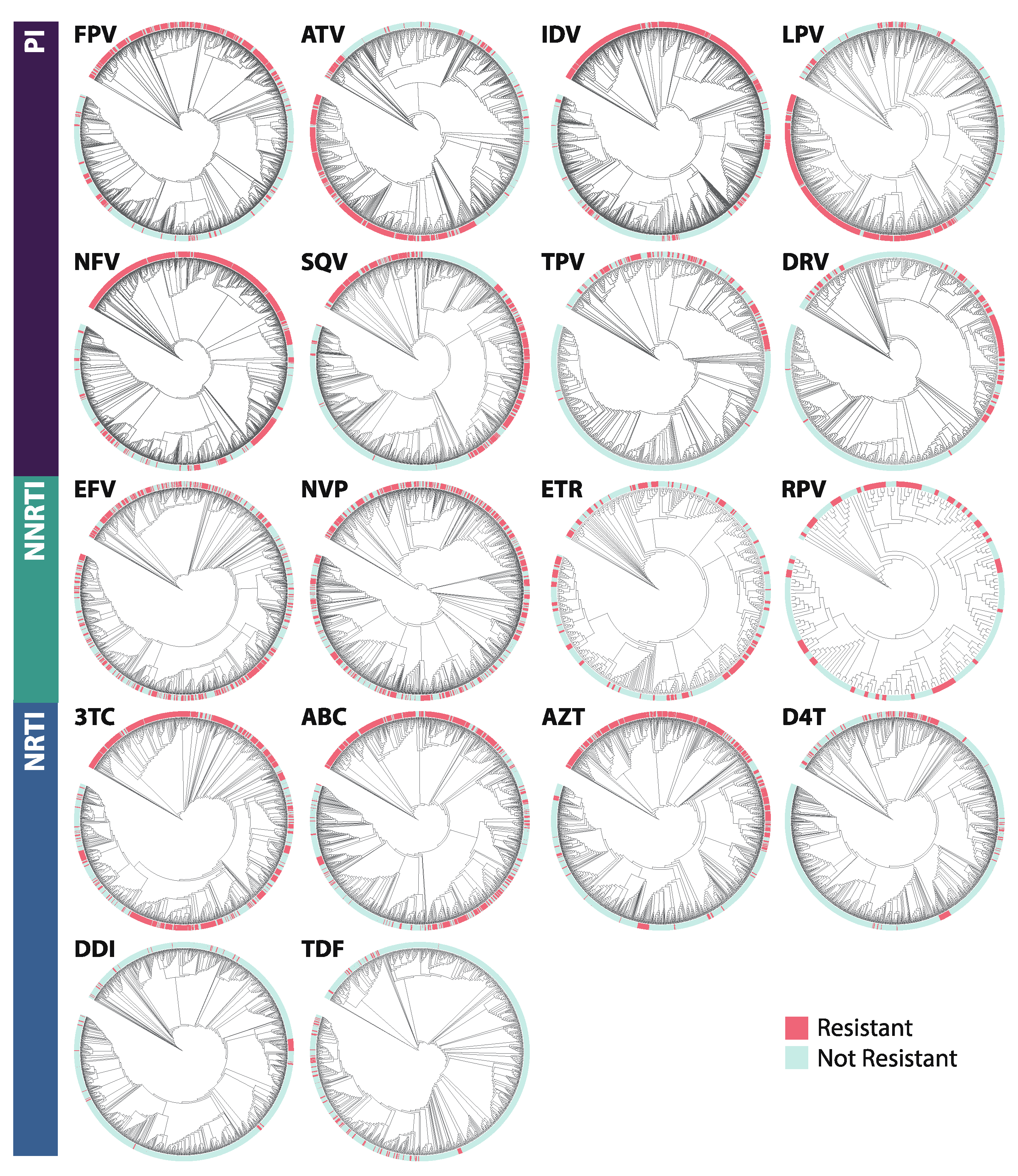
| Drug | Drug Class | No. Sequences | Sequence Length | (%) Resistant |
|---|---|---|---|---|
| FPV | PI | 1444 | 99 | 36.5 |
| ATV | PI | 987 | 99 | 43.4 |
| IDV | PI | 1491 | 99 | 43.7 |
| LPV | PI | 1267 | 99 | 44.7 |
| NFV | PI | 1532 | 99 | 52.8 |
| SQV | PI | 1483 | 99 | 37.6 |
| TPV | PI | 696 | 99 | 17.8 |
| DRV | PI | 605 | 99 | 21.5 |
| All PI | 2112 | 99 | 41 | |
| EFV | NNRTI | 1471 | 240 | 41.5 |
| NVP | NNRTI | 1478 | 240 | 47.8 |
| ETR | NNRTI | 481 | 240 | 28.7 |
| RPV | NNRTI | 181 | 240 | 32 |
| All NNRTI | 1772 | 240 | 42 | |
| 3TC | NRTI | 1270 | 240 | 58.3 |
| ABC | NRTI | 1293 | 240 | 46.1 |
| AZT | NRTI | 1283 | 240 | 41.8 |
| D4T | NRTI | 1291 | 240 | 13 |
| DDI | NRTI | 1291 | 240 | 5.3 |
| TDF | NRTI | 1025 | 240 | 8.8 |
| All NRTI | 2129 | 240 | 40.4 | |
| MLP | ||||||||
|---|---|---|---|---|---|---|---|---|
| Class | Accuracy | Loss | TPR | TNR | FPR | FNR | AUC | F1 |
| PI | 0.826 [0.039] | 0.406 [0.058] | 0.813 [0.041] | 0.834 [0.061] | 0.166 [0.061] | 0.187 [0.041] | 0.9 [0.009] | 0.732 [0.135] |
| NNRTI | 0.706 [0.095] | 0.586 [0.143] | 0.662 [0.140] | 0.718 [0.105] | 0.282 [0.105] | 0.338 [0.140] | 0.805 [0.006] | 0.596 [0.158] |
| NRTI | 0.795 [0.061] | 0.470 [0.150] | 0.725 [0.112] | 0.807 [0.081] | 0.193 [0.081] | 0.275 [0.112] | 0.895 [0.024] | 0.593 [0.236] |
| BRNN | ||||||||
| Class | Accuracy | Loss | TPR | TNR | FPR | FNR | AUC | F1 |
| PI | 0.912 [0.032] | 0.290 [0.087] | 0.890 [0.065] | 0.919 [0.028] | 0.081 [0.028] | 0.110 [0.065] | 0.965 [0.014] | 0.860 [0.106] |
| NNRTI | 0.884 [0.104] | 0.334 [0.247] | 0.829 [0.165] | 0.914 [0.088] | 0.086 [0.088] | 0.171 [0.165] | 0.83 [0.021] | 0.836 [0.180] |
| NRTI | 0.896 [0.030] | 0.357 [0.094] | 0.751 [0.168] | 0.910 [0.029] | 0.090 [0.029] | 0.249 [0.168] | 0.89 [0.02] | 0.698 [0.220] |
| CNN | ||||||||
| Class | Accuracy | Loss | TPR | TNR | FPR | FNR | AUC | F1 |
| PI | 0.919 [0.019] | 0.745 [0.204] | 0.865 [0.081] | 0.939 [0.013] | 0.061 [0.013] | 0.135 [0.081] | 0.968 [0.007] | 0.871 [0.088] |
| NNRTI | 0.911 [0.048] | 0.614 [0.219] | 0.845 [0.099] | 0.945 [0.029] | 0.055 [0.029] | 0.155 [0.099] | 0.945 [0.012] | 0.861 [0.097] |
| NRTI | 0.920 [0.035] | 0.805 [0.277] | 0.743 [0.182] | 0.940 [0.040] | 0.060 [0.040] | 0.257 [0.182] | 0.927 [0.016] | 0.757 [0.163] |
© 2020 by the authors. Licensee MDPI, Basel, Switzerland. This article is an open access article distributed under the terms and conditions of the Creative Commons Attribution (CC BY) license (http://creativecommons.org/licenses/by/4.0/).
Share and Cite
Steiner, M.C.; Gibson, K.M.; Crandall, K.A. Drug Resistance Prediction Using Deep Learning Techniques on HIV-1 Sequence Data. Viruses 2020, 12, 560. https://doi.org/10.3390/v12050560
Steiner MC, Gibson KM, Crandall KA. Drug Resistance Prediction Using Deep Learning Techniques on HIV-1 Sequence Data. Viruses. 2020; 12(5):560. https://doi.org/10.3390/v12050560
Chicago/Turabian StyleSteiner, Margaret C., Keylie M. Gibson, and Keith A. Crandall. 2020. "Drug Resistance Prediction Using Deep Learning Techniques on HIV-1 Sequence Data" Viruses 12, no. 5: 560. https://doi.org/10.3390/v12050560
APA StyleSteiner, M. C., Gibson, K. M., & Crandall, K. A. (2020). Drug Resistance Prediction Using Deep Learning Techniques on HIV-1 Sequence Data. Viruses, 12(5), 560. https://doi.org/10.3390/v12050560


