Productivity and Costs of Two Beetle-Kill Salvage Harvesting Methods in Northern Colorado

Abstract

Two ground-based timber harvesting methods have been commonly used for beetle-kill salvage treatments after a bark beetle epidemic in northern Colorado. A “lop and scatter” method uses a mobilized stroke delimber to delimb and buck trees at the stump, leaving tree tops and limbs on the forest floor, while a whole-tree harvesting method brings the entire tree to the landing where it is delimbed and bucked, and thus produces logging residue piles at the landing as a byproduct. We conducted a detailed comparative time study of the two harvesting methods to develop productivity and cost models and compared the performance of the two methods under various site conditions. We applied the productivity and cost models to lodgepole pine forest stands totaling 3400 hectares of the Colorado State Forest State Park to estimate salvage harvesting costs for each forest stand and identify the least costly harvesting options. The results show that the estimated stump-to-truck timber production costs were $30.00 per oven dry ton (odt) for lop and scatter and $23.88 odt⁻¹ for the whole-tree method in our study harvest unit. At the forest level, the estimated average stump-to-truck costs were $54.67 odt⁻¹ and $56.95 odt⁻¹ for lop and scatter and whole-tree harvesting, respectively. Skidding distance and downed trees affect the harvesting costs of both methods, but their influence appears to be more significant on the whole-tree method.

1. Introduction

Since 1996, approximately 1.37 million hectares of coniferous forests in Colorado have been affected by eruptive populations of bark beetles [1]. Although the dead trees resulting from the pine beetle epidemic represent a vast, high-density biomass resource for wood products, bioenergy and bio-based products, there exist many economic and environmental uncertainties with respect to the harvesting of beetle-killed stands, as well as downstream logistics and product markets. These uncertainties become especially apparent when one attempts to market and utilize low-value, less-merchantable woody biomass, including logging residues and logs from severely damaged trees [2,3].

There are a number of past studies that investigated forest biomass utilization to improve the efficiency of biomass production and associated supply chain logistics. Some topics include harvesting, processing and transportation efficiency [4,5,6,7], supply chain planning [8,9], and feedstock quality control for various energy products [10,11]. Most of the existing studies, however, assume that logging residues are a necessary byproduct of forest management treatments and thus are readily available at the landing with zero or low stumpage and harvesting costs.

In Colorado, two harvesting methods have been commonly used in beetle-kill salvage treatments: lop and scatter (LS) and whole-tree harvesting (WT). Depending on the choice of harvesting method, logging residues and non-merchantable roundwood may or may not be a readily available byproduct of salvage treatments. In LS, trees are delimbed and bucked at the stump, with an intention to leave all non-merchantable material on the forest floor. Although there may be some positive effects of such biomass retention on soil resources and seedling growth [12], this material is not available for utilization unless subsequent biomass collection operations are carried out at significant additional cost. In contrast, WT removes trees without processing at the stump and typically produces roadside logging residue piles because delimbing and bucking occur at the landing. Though these roadside residues are conventionally considered “free” of harvesting and stumpage costs because they are a necessary byproduct of the WT system, this may not be the case if there is a choice between WT and LS. If WT results in higher net costs than LS, concentrating logging residues at the landing incurs an opportunity cost. When LS is possible, this cost must be taken into account.

It is perceived that the WT method may have higher efficiency in delimbing than LS because delimbers do not need to move around within the harvest unit [13,14]. However, this efficiency gain normally comes with an efficiency loss in primary transport of whole trees from the stump to the landing, especially where skidding distance is long [15,16]. Despite the importance of this tradeoff in determining costs, no clear and objective comparisons on system productivity and costs have been made between the two methods. In practice, aside from conventional wisdom, there is almost no empirical information available to guide the choice between LS and WT when biomass utilization is possible. A better understanding of the costs and productivity of each method is needed in order for forest managers to properly assess the costs of logging operations and the potential for biomass utilization from the salvage of beetle-killed stands. This new knowledge will lead to better-informed salvage harvest decisions, and more efficient production of both biomass and timber products.

This study aims to develop comparable productivity and cost models for the two beetle-kill salvage harvest methods through detailed operational time studies. Our study provides insights into how stand and operational conditions affect the performance of each harvesting method to help forest managers properly evaluate logging residue costs and make informed decisions on beetle-kill stand management for maximum economic and environmental benefits. For demonstration purposes, we applied our productivity and cost models to lodgepole pine stands covering about 3400 hectares of the Colorado State Forest State Park located in northern Colorado. We estimated salvage harvesting costs for each stand and identified the least costly harvesting option to assess the potential costs of logging residues.

2. Materials and Methods

2.1. Study Harvest Unit and Salvage Harvest Methods

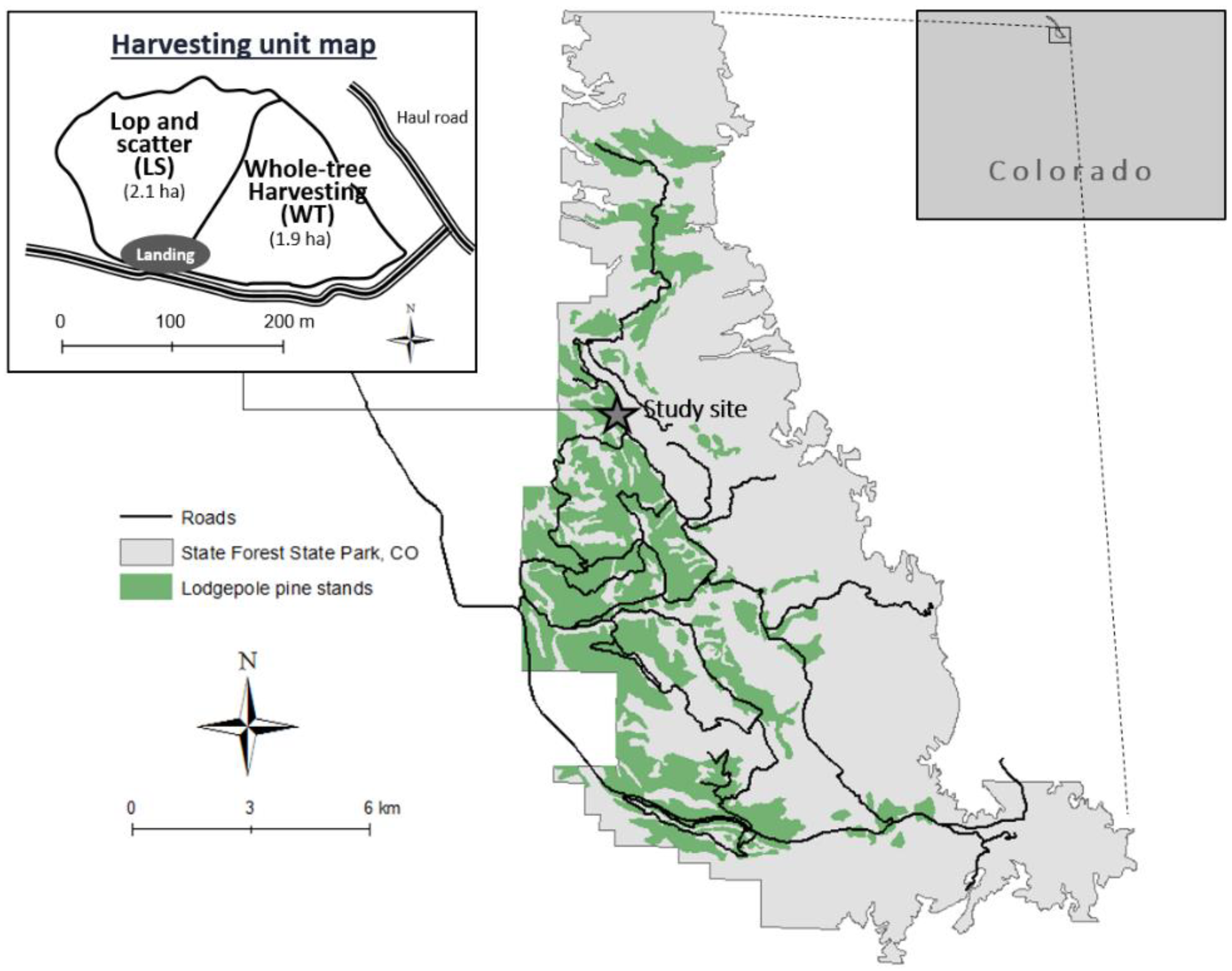
In collaboration with the Colorado State Forest Service, we identified a 4.0-ha lodgepole pine (Pinus contorta Dougl. ex. Loud. var. latifolia) clearcut unit in the Colorado State Forest State Park in northern Colorado (40°35′59″ N, 106°00′27″ W), and conducted a detailed time study on forest operations. The harvest unit is located on relatively flat terrain, and was infested by the mountain pine beetle beginning in 2008. A clearcut salvage harvest was prescribed based on the high level of mortality in this unit. We split the unit into two approximately equal halves, and applied the LS and WT harvesting methods side by side for a fair comparison (Figure 1). The harvest unit was cruised for inventory prior to clearcut treatment using a systematic fixed plot sampling method with a 5% sampling intensity. For stand inventory, we measured trees with diameter at breast height (dbh) larger than 12.7 cm (

Table 1. Stand characteristics of the study harvest unit.

Characteristics	Harvesting Unit
	Lop and Scatter (LS)	Whole-Tree Harvesting (WT)	Combined
Area (ha)	2.1	1.9	4.0
Mean dbh (cm)	22.4	22.4	22.4
Mean height (m)	18.3	19.6	19.1
Basal area (m2 ha−1)	33.3	34.6	33.9
Trees per hectare	818	865	841
Mortality (%)	39.5	47.3	43.5

).

The study harvest unit was clearcut in December 2015 using ground-based harvesting equipment. The same equipment and machine operators were employed for both harvesting methods to minimize the influence of equipment and operator variability on productivity (

Table 2. Harvesting equipment purchase price, utilization rate, and machine hourly rate used for cost analysis in this study.

Machine (Make/Model)	Purchase Price ($)	Utilization Rate * (%)	Machine Rate ($ SMH−1) †
Feller‒buncher (TimberPro TL-735-B §)	395,000	60	135.93
Stroke delimber (Timberline SDL2 ¶)	355,000	65	116.58
Skidder (Tigercat 615C ‡)	219,000	60	92.86
Grapple loader (Barko 495ML Magnum б)	205,000	65	81.15

* Adapted from [17]. ^† Scheduled machine hour (SMH). ^§ TimberPro Inc., Shawano, WI, USA. ^¶ DDI Equipment, Whitewater, CO, USA. ^‡ Tigercat Industires Inc., E. Brantford, ON, Canada. ^б Barko Hydraulics, LLC, Superior, WI, USA.

). In both methods, a feller‒buncher was used to cut down trees and put them into bunches within the unit. Two stroke delimbers were used to top, delimb and buck trees, either at the stump for LS or at the landing for WT, while a grapple skidder transported either whole trees (WT) or log lengths (LS) to the landing. The major difference between the two harvesting methods is the sequence of machine operations and delimber locations. In WT, the skidder brought whole trees to the landing after the feller‒buncher made tree bunches in the unit, and then the delimbers, stationed at the landing, processed the trees into logs, which created slash piles at the landing. In LS, following the feller‒buncher the delimbers moved to each tree bunch location in the unit and processed trees at the bunch location. The skidder then brought only merchantable logs to the landing, with all slash left on the unit. For both methods, the same loader was used to sort and load logs onto trucks at the landing (Figure 2). Because of the relatively small size, most of the harvested trees yielded only one log of an average length of 12 m. Depending on the small-end diameter and defects, logs were sorted into three products: saw logs, pulp and firewood.

2.2. Detailed Time Study and Cycle Time Regression Models

Detailed time study data were collected to estimate machine productivity using standard work study techniques [17,18]. Based on preliminary observations, we selected independent variables for each machine that would likely affect machine productivity (

Table 3. Time elements and variables measured during detailed time study for the lop and scatter (LS) and whole-tree harvesting (WT) methods.

Equipment	Time Element per Cycle	Variables Measured
Feller‒buncher	Move to trees	Travel distance (m)
	Position the felling head and felling	No. of standing trees
	Bunch	No. of downed trees
Stroke delimber	Move and reposition *	Delimber movement (0 = not moving, 1 = moving)
	Grapple	No. of live and dead trees
	Delimb, top and process
Skidder	Travel empty	Travel distance (m)
	Position and grapple	No. of logs or whole trees †
	Travel loaded	Travel distance (m)
	Unload
Grapple loader	Grapple	No. of logs
	Sort or load	Loader activity (0 = sorting, 1 = loading)

* Delimber movement was measured and recorded only in LS because the delimber is positioned on the landing for WT. ^† The number of processed logs were measured in LS, while the number of whole trees was measured in WT.

). During field data collection, we recorded the delay-free cycle times of all machine operations using stopwatches and measured independent variables in each machine cycle. In order to analyze the effects of dead trees on machine cycle times and productivity, we classified trees into ‘live’ and ‘dead’ for delimbing, and ‘standing’ and ‘downed’ for cutting and bunching operations [19]. Feller‒buncher movement between trees in both methods and delimber movement between tree bunches in LS were measured by counting the number of machine track rotations, which was later converted to linear distance based on track length. Loader activities were categorized into two main tasks (i.e., sorting and loading), and machine cycle times were measured separately for each task. For the skidder, empty and loaded travel distances were measured using a GPS receiver (Columbus VGPS-900, Victory Tech Co., Ltd., Fuzhou, China) located inside the machine cabin. The GPS receiver was set to record tracking points at every second.

Predictive equations of delay-free machine cycle times were developed using the ordinary least squares regression technique. For each machine, cycle times beyond three standard deviations from the mean value were classified as outliers and excluded from the analysis. Two-thirds of the cycle time data were randomly selected for model construction, while the remaining one-third of the data were used for model validation. A paired t-test was used to compare predicted and observed values and identify any statistical differences during model validation.

For the feller‒buncher and the loader, we blended the data from both harvesting methods into one predictive equation because there was no difference in machine operations between the two methods. For the delimber and the skidder, separate cycle time regression equations were built for each harvesting method because of different equipment movement and log handling in each method. A binary variable was used to indicate the presence of delimber movement in each delimber cycle in LS (Table 3). All statistical analyses were carried out in R software [20], and a small p-value (<0.05) was considered to be statistically significant.

2.3. Harvesting System Productivity and Production Costs

The production amount in a machine cycle was normalized to oven dry ton (odt, a ton of woody material at 0% moisture content) by applying the average log dry weight to the number of logs produced. The average truck load in green weight was obtained from the mill trip tickets, which provide scale measures of gross and net truck weight for each truck cycle. The average log dry weight was estimated based on the observed average number of logs per truck load, the ratio of live and dead trees in the harvest unit, and the average moisture contents of live and dead trees obtained from the previous study conducted at the Colorado State Forest State Park [21].

Using the average cycle time and timber production per cycle, machine productivity was estimated in odt per scheduled machine hour (SMH). For each system, the bottleneck machine was identified, and the system productivity was determined based on the bottleneck productivity, assuming all the machines work simultaneously, but are constrained by the bottleneck [19].

Hourly costs of the individual machines were estimated based on 2000 SMH per year [22] using STHARVEST [23] with updated machine purchase prices and operator wages for the region. We also adapted data from published rates in the literature [17] for machine life and depreciation, salvage value, machine utilization rate, fuel consumption rate, and repair and maintenance costs. An interest rate of 10% and an insurance and tax rate of 4% were used. Fuel cost was estimated based on off-road diesel costs for the region and the cost of lubrication and oil was estimated at 37% of the fuel cost. Finally, we estimated system production cost ($ odt⁻¹) as the ratio of total machine hourly costs ($ SMH⁻¹) to system productivity (odt SMH⁻¹).

2.4. Slash Pile Measurement and Biomass Leakage Estimation

The WT method produces logging residues in the form of slash piles at the landing. We measured the dimensions and calculated the volume of each slash pile using a TruPulse laser range finder (Laser Technology, Inc., Centennial, CO, USA) [24], and then converted the volume to dry weight using a packing ratio of 10% [25] and a bulk density of 76.7 kg m⁻³ [26].

The amount of biomass cut but unrecovered during primary transportation (i.e., biomass leakage) in WT was estimated by subtracting the amount in slash piles measured at the landing from the estimated logging residue portion of standing trees. The logging residue portion of standing trees (i.e., tree tops, limbs, and foliage) was estimated using the allometric equations specifically developed for both live and dead lodgepole pine in the region [21]. The volume of tree tops had to be adjusted for this study because [21] considered a tree top as the tree portion above 10-cm diameter, whereas the practice in the study harvest unit was to remove tree tops at 18-cm diameter due to timber product specifications for markets in the region [27]. Tree length between 10-cm and 18-cm diameters was estimated using the Kozak equation [28], and the biomass volume of this portion was estimated using the Smalian formula [29]. The volume was then converted to green weight of biomass by multiplying a wood density of 371 kg m⁻³ [30], and converted subsequently to dry weight using the average water contents in live and dead trees and the observed proportions of live and dead trees from the study harvest unit. These calculations adjusted allometric outputs to allow for the biomass between 10-cm diameter and 18-cm diameter to be included in the biomass portion of the removal, as was the practice in the field.

2.5. Model Application

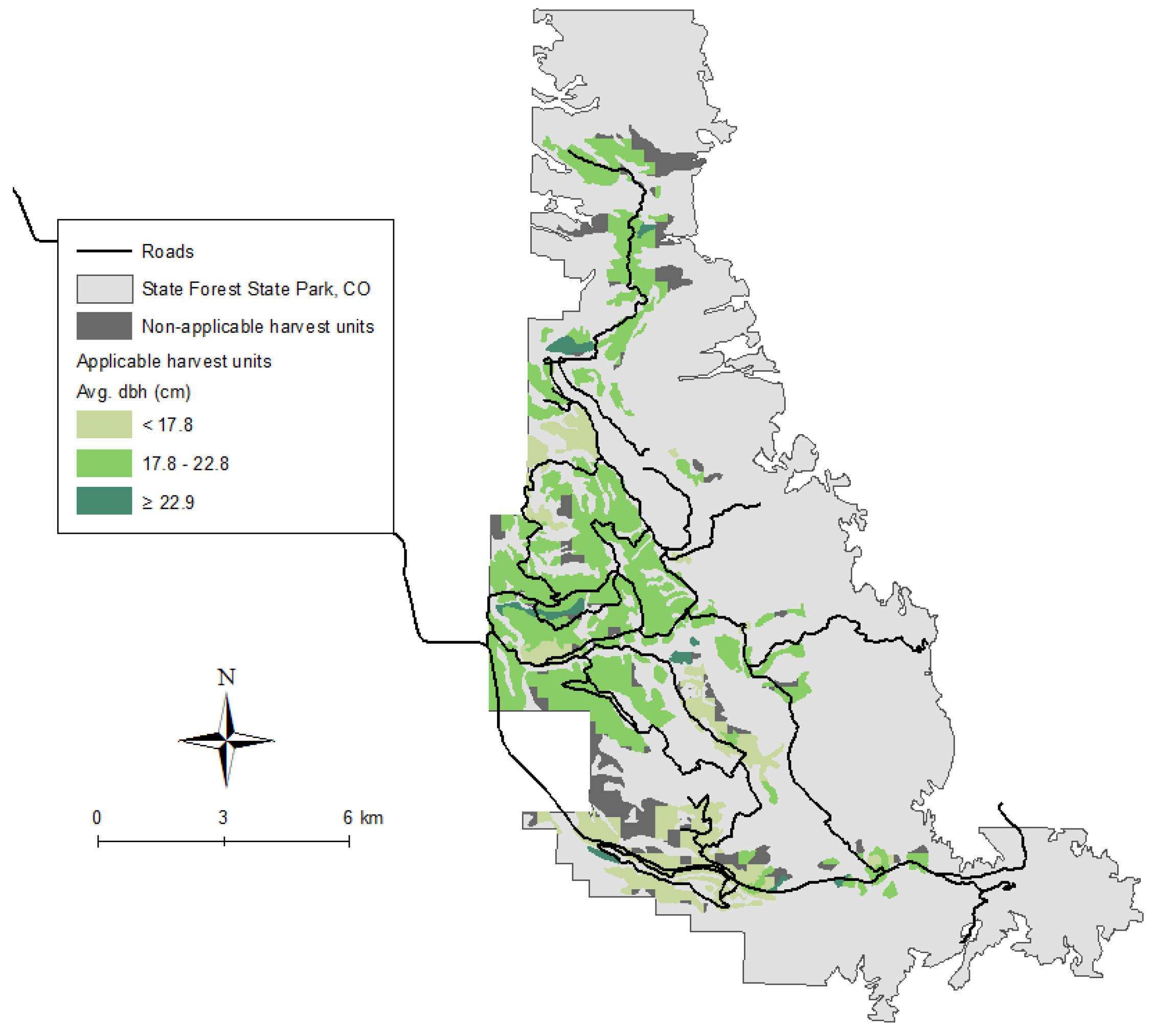
We applied the harvesting system productivity and cost models developed in this study to lodgepole pine stands in the Colorado State Forest State Park to identify the least costly beetle-kill salvage harvest options for each stand and quantify the potential costs of harvesting logging residues under the lowest cost constraints. First, we divided beetle-infested lodgepole pine stands into grids of 8 hectares using ArcGIS [31] to generate manageable harvest units. We then excluded stands that were steeper than a 30% slope because ground-based harvesting may not be applicable on steep slopes. We also excluded areas where the distance from the grid centroid to the nearest road exceeds 610 m, assuming it is not economically feasible to skid logs over what is considered a very long distance in this region. As a result, we identified approximately 3400 hectares of lodgepole pine stands in the Colorado State Forest State Park as potential treatment areas (Figure 3).

Timber production cost at each harvest unit was predicted using our productivity and cost models developed for LS and WT based on the estimated empty and loaded skidding distances, and the average dry log weight for the unit. The average empty and loaded distances observed from the study unit were slightly different; empty distance was slightly longer than loaded distance due to machine turnarounds. For model applications, empty and loaded skidding distances were estimated using the average skidding distance but further adjusted accordingly to reflect the differences observed in the field. The average skidding distance was estimated using ArcGIS as the distance between the unit centroid and the nearest road. To be clear, the threshold for maximum skidding distance of 610 m from grid centroid to the nearest road used in harvest unit designation is well beyond the maximum skidding distance observed during the field study, which required us to extrapolate the relationships observed over shorter skidding distances to more distant units. Though not ideal, we believe this is appropriate in this case because: (1) the emphasis here is on exploring tradeoffs between the two harvest methods, especially those related to skidding distance, (2) we could not identify any theoretical, empirical, or anecdotal reason why the observed relationship would not hold over longer skidding distances, (3) in this application more distant units do not vary from closer units in any significant attribute, such as topography or hydrology, and (4) our assumption of a positive linear relationship between skidder cycle time and skidding distance over a wide range of distances has been proven in previous studies [32,33,34].

The average dry log weight was estimated using the mean stand dbh provided by the Colorado State Forest Service [35] and the data on log dry weight obtained from the study harvest unit. The proportions of dead and downed trees were assumed to remain the same as those observed in the study harvest unit.

After we estimated unit production costs of timber for each harvest unit using the two harvesting methods, the least costly harvesting method was selected as the preferred option for the unit. We assumed that logging residues could be obtained for zero harvest and stumpage cost as a byproduct of salvage harvest when WT is the least costly option, but otherwise there would be actual costs associated with logging residue harvesting and collection. In the latter case, the difference between WT and LS harvesting costs (i.e., the cost of using WT when LS is the lower cost option) was calculated and used as a surrogate measure of the actual marginal cost of logging residue production by harvesting unit.

3. Results

3.1. Machine Cycle Times

The total number of observed cycle times varied widely among different machines ranging from 34 for the skidder in LS to 873 for the feller‒buncher (

Table 4. Mean delay-free cycle times observed by harvesting equipment in lop and scatter (LS) and whole-tree harvesting (WT).

Equipment	Number of Cycle Times		Machine Cycle Time
	Observed	Outliers	n	Mean (s cycle−1)	Std * (s cycle−1)
Feller‒buncher (LS + WT)	873	10	863	19.31	6.88
Stroke delimber (LS)	571	4	567	42.30	16.39
Stroke delimber (WT)	391	5	386	41.34	12.55
Skidder (LS)	34	2	32	209.34	56.21
Skidder (WT)	37	1	36	239.78	43.73
Grapple loader (LS + WT)	438	7	431	37.82	16.18

* Standard deviation.

). A total of 29 cycles were classified as outliers and removed from the analysis. On average, the feller‒buncher took 19.3 s to complete its cycle without delays. The stroke delimber took slightly more time to complete its cycle in LS than WT mainly because the machine had to move between tree bunches in LS. In contrast, the grapple skidder consumed more time in WT to transport whole trees than in LS where it transported processed logs. The grapple loader’s average cycle time was 37.8 s for its sorting and loading activities (Table 4).

The existence and condition of dead trees can affect machine and system productivity in beetle-kill salvage harvest, with higher levels of downed trees associated with longer cycle times and lower productivity [19]. Our results show that the feller‒buncher took substantially more time over handling downed trees (28.0 s) or standing and downed trees together (29.3 s) compared to standing trees only (18.8 s) (

Table 5. Observed machine cycle times of feller‒buncher and stroke delimber based on the tree conditions in beetle-kill salvage harvesting (LS: lop and scatter; WT: whole-tree harvesting).

Machine	Observed Machine Cycle Time (s cycle−1)
	Category	n	Mean	Std	Group *
Feller‒buncher	Standing trees only	815	18.79	6.47	a
	Downed trees only	30	27.99	8.03	b
	Mixed with downed trees	18	29.28	7.39	b
	Combined	863	19.31	6.88
Stroke delimber (LS)	Live trees only	209	42.07	15.13	c
	Dead trees only	341	41.90	17.02	c
	Mixed	17	53.24	15.65	d
	Combined	567	42.30	16.39
Stroke delimber (WT)	Live trees only	126	41.98	11.95	e
	Dead trees only	194	38.94	11.96	f
	Mixed	66	47.18	13.44	g
	Combined	386	41.34	12.55

* Duncan’s Multiple Range test was used to provide a pair-wise comparison of tree group means. The same letter indicates that means are not significantly different (p > 0.05).

). For the delimber, it took a shorter time to process dead trees than live trees in both methods, probably due to fewer branches to delimb on dead trees, but the difference was only statistically significant in WT. However, when the delimber processed a mix of dead and live trees, the average cycle time increased by 27% and 12% in LS and WT, respectively, compared to processing only live trees.

3.2. Delay-Free Cycle Time Regression Models

Table 6. Delay-free cycle time regression models for feller‒buncher, delimber, skidder, and grapple loader used in lop and scatter (LS) and whole-tree harvesting (WT). Cycle times are in seconds (s). A paired t-test was used for model validation against observed data.

Machine	Parameter	Variable		Estimate	SE	t	p-Value	Model adj. R2	Model p-Value	t-Test (p-Value)
		Range	Mean
Feller‒buncher	Intercept			10.140	0.614	16.50	<0.01	0.4329	<0.01	0.1980
	No. of standing trees	0−4	1.84	3.709	0.296	12.54	<0.01
	No. of downed trees	0−2	0.06	13.082	0.870	15.04	<0.01
	Travel distance (m)	0−23.2	1.7	0.989	0.080	12.29	<0.01
Stroke delimber (LS)	Intercept			30.177	1.524	19.797	<0.01	0.3848	<0.01	0.8118
	No. of live trees	0−8	0.60	6.209	1.007	6.164	<0.01
	No. of dead trees	0−4	0.74	5.941	1.195	4.972	<0.01
	Move and reposition *	0−1	0.13	30.254	2.061	14.679	<0.01
Stroke delimber (WT)	Intercept			30.765	1.522	20.219	<0.01	0.1898	<0.01	0.3887
	No. of live trees	0−5	0.76	6.624	0.913	7.252	<0.01
	No. of dead trees	0−5	0.92	5.729	0.961	5.963	<0.01
Skidder (LS)	Intercept			71.779	24.641	2.913	<0.01	0.6430	<0.01	0.4362
	No. of logs	9−32	20.16	3.033	1.295	2.342	<0.05
	Empty distance (m)	21.3−317.0	151.3	0.493	0.196	2.513	<0.05
	Loaded distance (m)	12.2−225.6	129.0	0.053	0.268	0.199	0.845
Skidder (WT)	Intercept			25.125	47.530	0.529	0.603	0.5976	<0.01	0.3605
	No. of trees	9−40	21.89	1.881	0.984	1.913	0.070
	Empty distance (m)	82.3−216.4	163.6	0.632	0.325	1.944	0.066
	Loaded distance (m)	42.7−213.4	139.7	0.477	0.241	1.983	0.061
Loader	Intercept			22.006	1.892	11.629	<0.01	0.2033	<0.01	0.1254
	No. of logs	1−14	3.28	3.739	0.471	7.937	<0.01
	Activity type †	0−1	0.30	8.248	1.794	4.597	<0.01

* Delimber movement (0 = not moving, 1 = moving). ^† Loader activity (0 = sorting, 1 = loading).

shows the range and mean of independent variables and delay-free cycle time regression equations developed for each machine. On average, the feller‒buncher moved about 1.7 m per cycle to reach trees. There were only a few downed trees observed (about 3% of total cut trees), but the results showed one downed tree increases the feller‒buncher cycle time by 13.1 s, which significantly reduced the operational efficiency of the machine. In LS, the stroke delimber moved and repositioned about every nine delimbing cycles. The delimber processed 1.34 trees per cycle on average in LS, whereas it processed about 1.68 trees per cycle in WT, which is over 25% more. Compared to LS, the delimber in WT was able to grab as many trees as possible in each cycle from a large stack of trees at the landing, which the skidder continuously supplied during operations. The skidder transported 20.2 logs per cycle in LS and 21.9 whole trees in WT, on average. The loader moved 3.3 logs per cycle, while spending 70% and 30% of its total productive time on sorting and loading, respectively.

Most independent variables were significant (p ≤ 0.05) except for those in the skidder cycle time models. The loaded distance was not a significant variable in LS, and all predictor variables in the WT model were only significant at 10% significance level (p ≤ 0.10). These high p-values of empty and loaded distance variables were mainly caused by the high correlation between the two variables. Although the regression models we tested with only one distance variable showed the significance of the distance variable (p ≤ 0.05), we chose to keep two distance variables in our regression model because the performance of both models (one with two distance variables and the other with only one distance variable) was similar in terms of Akaike information criterion (AIC) and Bayesian information criterion (BIC) metrics, yet we were able to preserve more information with two variables. For all regression models, a paired t-test was performed for model validation against observed data. The test results indicate that the predicted cycle time values were not statistically different from the observed values (p > 0.05).

3.3. Productivity and Costs of Two Beetle-Kill Salvage Harvesting Methods

Most machines employed in LS had a similar productivity of about 25 odt SMH⁻¹ except for the two delimbers, with a combined productivity of 18.1 odt SMH⁻¹ (

Table 7. Productivity and costs of the lop and scatter (LS), and whole-tree harvesting (WT) methods.

Configuration/Machine	Machine
	Cycle Time (s cycle−1)	Cycle Rate (cycle SMH−1)	Turn Size (odt cycle−1)	Productivity (odt SMH−1)	Cost ($ odt−1)
Lop and scatter (LS)
Feller‒buncher	19.46	111.00	0.23	25.17	5.40
Stroke delimber *	42.23	55.41	0.16	18.10	12.89
Skidder	220.41	9.80	2.50	24.54	3.78
Grapple loader	36.74	63.68	0.39	24.84	3.26
LS system total	-	-	-	18.10	30.00
Whole-tree harvesting (WT)
Feller‒buncher	19.46	111.00	0.23	25.17	5.40
Skidder	228.23	9.46	2.50	23.69	3.92
Stroke delimber *	41.07	56.98	0.20	22.74	10.25
Grapple loader	36.74	63.68	0.39	24.84	3.26
WT system total	-	-	-	22.74	23.88

* Estimated for two delimbers.

). As a result, the unit production cost of LS was estimated at $30.00 odt⁻¹. The productivity of individual machines in WT ranged between 22.74 odt SMH⁻¹ for the two delimbers and 25.17 odt SMH⁻¹ for the feller‒buncher, indicating that the observed WT system was better balanced in productivity compared to LS. The system productivity of WT was also determined by the delimber that had the lowest productivity, and the unit production cost was estimated at $23.88 odt⁻¹, which was 20% lower than LS.

The performance of individual machines slightly differed between the two harvesting methods. The delimbers in LS had 20% lower productivity than those in WT, mainly due to smaller turn size and frequent machine movement. The average turn payload of the skidder was similar in both methods, but the machine took slightly longer per cycle in WT than in LS due to the longer average skidding distance and the extraction of whole trees. Our delay-free cycle time models also indicated that the average cycle time of the skidder was more sensitive to skidding distance in WT than in LS (Table 6).

3.4. Slash Pile Measurement and Biomass Leakage Estimation

The average volume of slash piles collected at the landing was approximately 1136 m³ in volume or 51 odt in weight (

Table 8. Slash pile measurement and leakage estimation in the study harvest unit.

Measurement	Estimated Value
Logging residues estimated * (odt) (A)	66
Additional residues estimated † (odt) (B)	43
Slash pile measured
Gross volume (m3)	1136
Net volume (m3) **	1022
Net dry weight (odt) (C)	51
Leakage
Amount (odt) (D = A + B − C)	58
Ratio (%) (D$/$(A + B))	53

* Estimated using the allometric equations developed by [21]. ^† Treetop component between 10 cm and 18 cm diameters estimated using the stem taper equation developed by [28]. ** After applying 10% packing ratio to gross volume [25].

). The maximum amount of logging residues that were theoretically recoverable without leakage was estimated at 109 odt (A + B in Table 8). This result showed that approximately 53% of logging residues could be lost before or during harvesting and extraction.

3.5. Model Application

The results of the application of LS and WT productivity and cost models to the lodgepole pine stands in the Colorado State Forest State Park show that the average costs of salvage harvest were $54.67 odt⁻¹ and $56.95 odt⁻¹ for LS and WT, respectively (

Table 9. (A) Lodgepole pine stand areas of the Colorado State Forest State Park assigned to whole-tree harvesting (WT) and lop and scatter (LS) methods based on harvesting costs. (B) The area, merchantable timber, and logging residues in each cost difference group between the two harvesting methods (WT − LS).

A			B
Harvesting Cost Groups ($ odt−1)	LS Area (ha)	WT Area (ha)	Cost Difference (WT − LS) ($ odt−1)	Area (ha)	Merchantable Timber (odt)	Logging Residues (odt)
<30	109.3	83.7	<−20	35.8	780.8	166.4
30–40	64.3	1024.6	−20–−10	1136.7	67,818.7	11,749.1
40–50	1544.8	555.5	−10–0	498.0	36,915.9	6134.1
50–60	669.0	328.5	0–10	315.8	22,987.2	3850.8
60–70	284.1	289.1	10–20	561.7	40,443.1	6837.7
70–80	188.0	196.5	≥20	522.5	34,719.5	5945.9
80–90	136.1	254.7
≥90	74.9	337.8

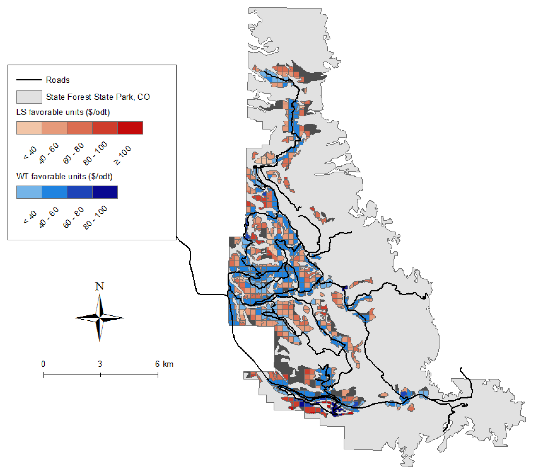
A). Figure 4 presents the economically preferred harvesting method selected for each unit after comparing the unit production costs of the LS and WT methods. Recall that skidding distance relationships observed in the field study were extrapolated to more distant units up to a maximum distance of 610 m between the grid centroid and nearest road. The results suggest that the average skidding distance was the critical factor that determined the more economical harvesting method. The WT method appeared to be less expensive in the areas close to the existing forest roads, whereas the LS method was less expensive in the areas relatively far from the existing roads (Figure 4). WT was chosen as the least costly option in about 54% of the total lodgepole pine stands analyzed in this study where the average skidding distance was 99 m (cost difference < 0 in Table 9B). Because WT was the least costly option in those areas, logging residues could be produced as a byproduct from salvage harvest. However, logging residues would not be available without additional costs in the rest of the lodgepole pine stands, which was about 46% of the total area. The average skidding distance of these areas was 377 m, and WT was more expensive than LS (cost difference > 0 in Table 9B). Our estimate showed the average additional marginal cost of timber production between WT and LS (i.e., WT − LS) in those areas was about $16.7 odt⁻¹. Considering the estimated amount of logging residues that could be possibly collected at the landing, the additional costs incurred by WT in timber production could result in the cost of logging residues as high as $98.32 per odt of logging residues in some harvest units.

4. Discussion

4.1. Effects of Dead Trees on Machine Performance and System Productivity

The productivity of machines varied when processing dead trees in the salvage harvest of beetle-killed stands. Feller‒buncher cycle time increased by up to 56% due to the handling of downed trees (Table 5). The number of downed trees generally increases as time passes since the beetle infestation due to rotted stems being more susceptible to breakage and wind throw [36]. As the proportion of downed trees increases within a stand, the feller‒buncher can be greatly impaired in productivity and create a bottleneck in the harvesting system [19]. 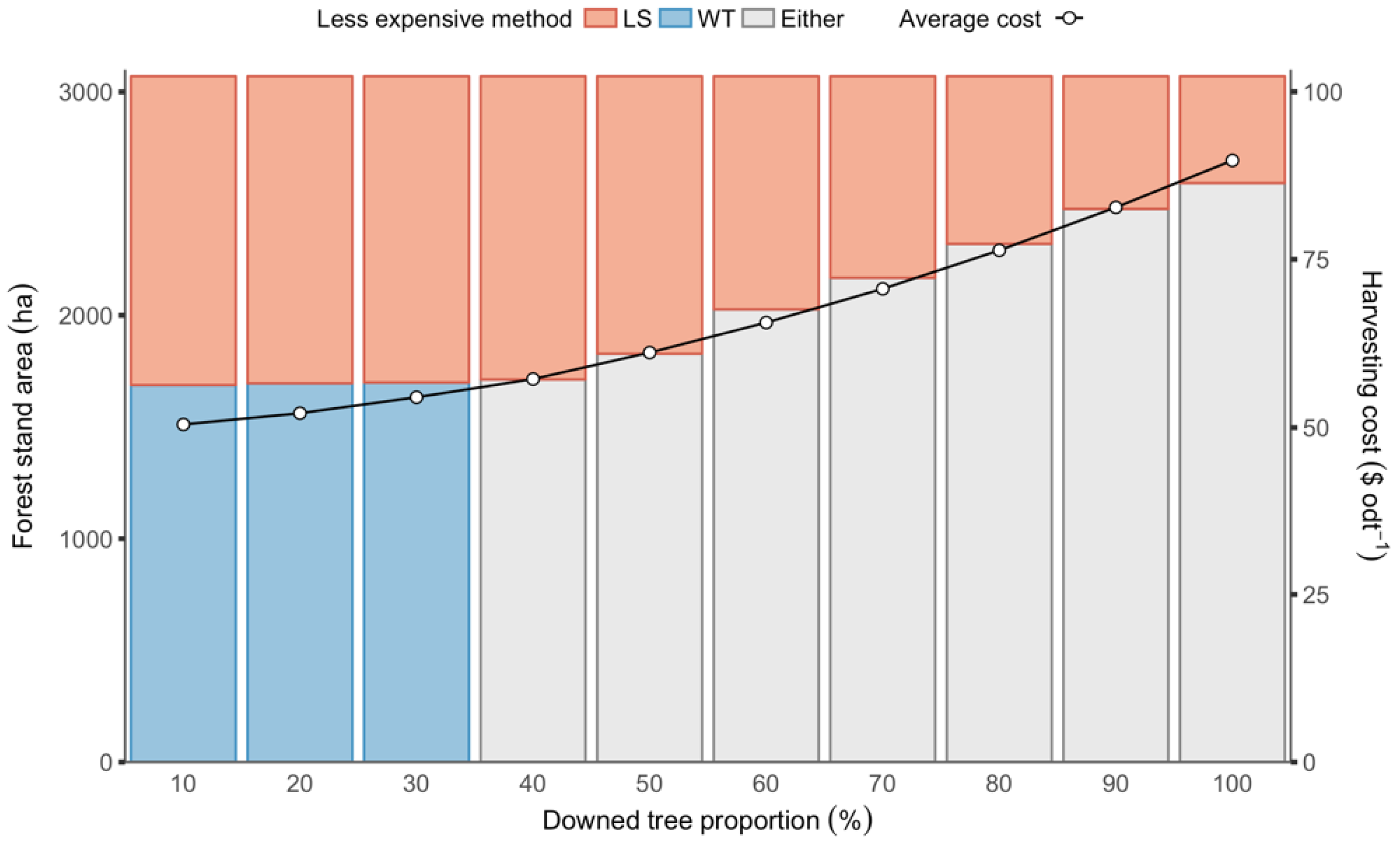The low productivity of the feller‒buncher and the resulting unbalanced harvesting system cause the increase of salvage harvesting costs in both LS and WT (Figure 5). Our analysis shows that WT remains a less expensive harvesting option for more than 50% of the study area when the downed tree proportion is less than 30%. However, if the downed tree proportion rises over 30% and the feller‒buncher becomes a system bottleneck, no area exists where WT exclusively becomes a less expensive method in this forest (Figure 5). On the contrary, our results show LS always remains a less expensive option for some areas across the range of downed tree proportions. This is because of the harvest areas requiring long-distance skidding, which makes LS less expensive than WT.

Our results imply that LS can be a more economically favorable harvesting method if salvage harvesting decisions and harvest timing are delayed for a long period of time, which results in a high proportion of downed trees in the forest. Such a delay is also likely to increase the production costs of timber and biomass and decrease the availability of logging residues due to the increased biomass leakage rate over time. This higher leakage is associated with older trees being more likely to break apart during felling and skidding, resulting in less recoverable slash making it to the landing and into slash piles.

4.2. Effects of Skidding Distance on Machine Performance and System Productivity

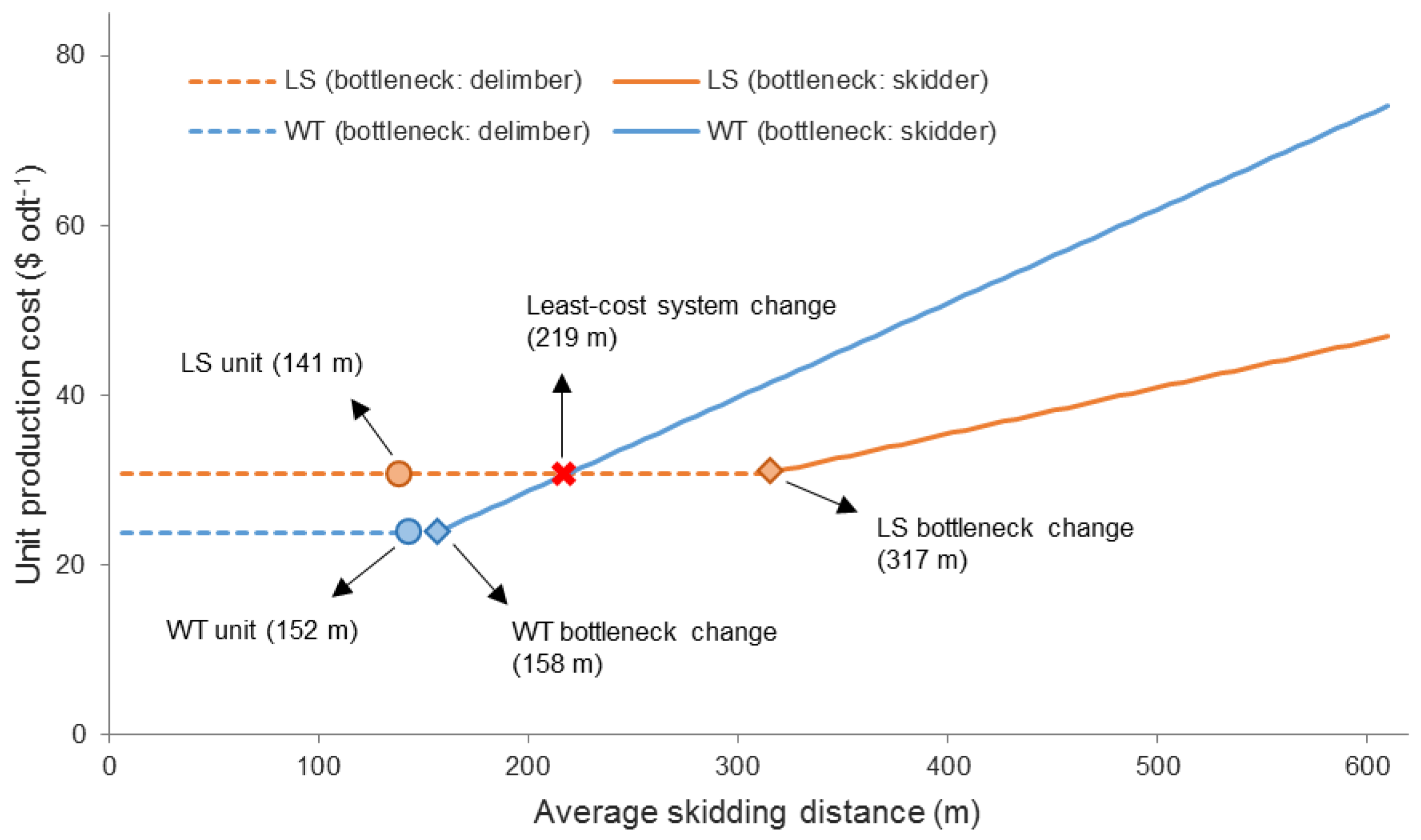
We performed a sensitivity analysis to evaluate how the bottleneck function changes in each harvesting method based on the average skidding distance. Because of the relatively short skidding distances in our study harvest unit, delimbing was the bottleneck function in both LS and WT. However, our sensitivity analysis results show that when the average skidding distance is longer than 158 m and 317 m for WT and LS, respectively, the skidder becomes the system bottleneck (Figure 6). This indicates that the unit production cost of the harvesting system is insensitive to skidding distance while the delimber is the bottleneck, but after the ‘tipping point’ in skidding distance is exceeded, the unit cost increases as skidding distance increases. The tipping point in WT appears to occur at a shorter distance than LS, but the unit production cost of WT is more sensitive to skidding distance than LS after the respective tipping point. The sensitivity analysis also indicates that there is a breakeven skidding distance between the two methods, assuming all other factors remain the same. When the average skidding distance is less than 219 m in our study harvest unit, WT becomes less expensive, whereas LS becomes a less expensive option when the skidding distance is greater than 219 m.

Figure 6 and associated conclusions should be viewed in light of the limitations of the study. Observed skidding distances in the field study were relatively short because of the economics of the harvest, which would not support long skidding distances given log prices at the time and the low quality of the beetle-killed logs. Therefore, extrapolation of observed relationships was required to project unit production costs for more distant units. Although extrapolation is not ideal, our assumption of a positive linear relationship between skidder cycle time and skidding distance over a wider range of distances is well supported by existing literature [32,33,34]. The accuracy of our cost projections may be affected by this limitation, but we believe our analysis can provide insights how skidding distance affects the productivity of the harvesting methods, suggesting harvesting cost trends beyond the current practices and observed operations.

4.3. Logging Residue Removal for Bioenergy Feedstock

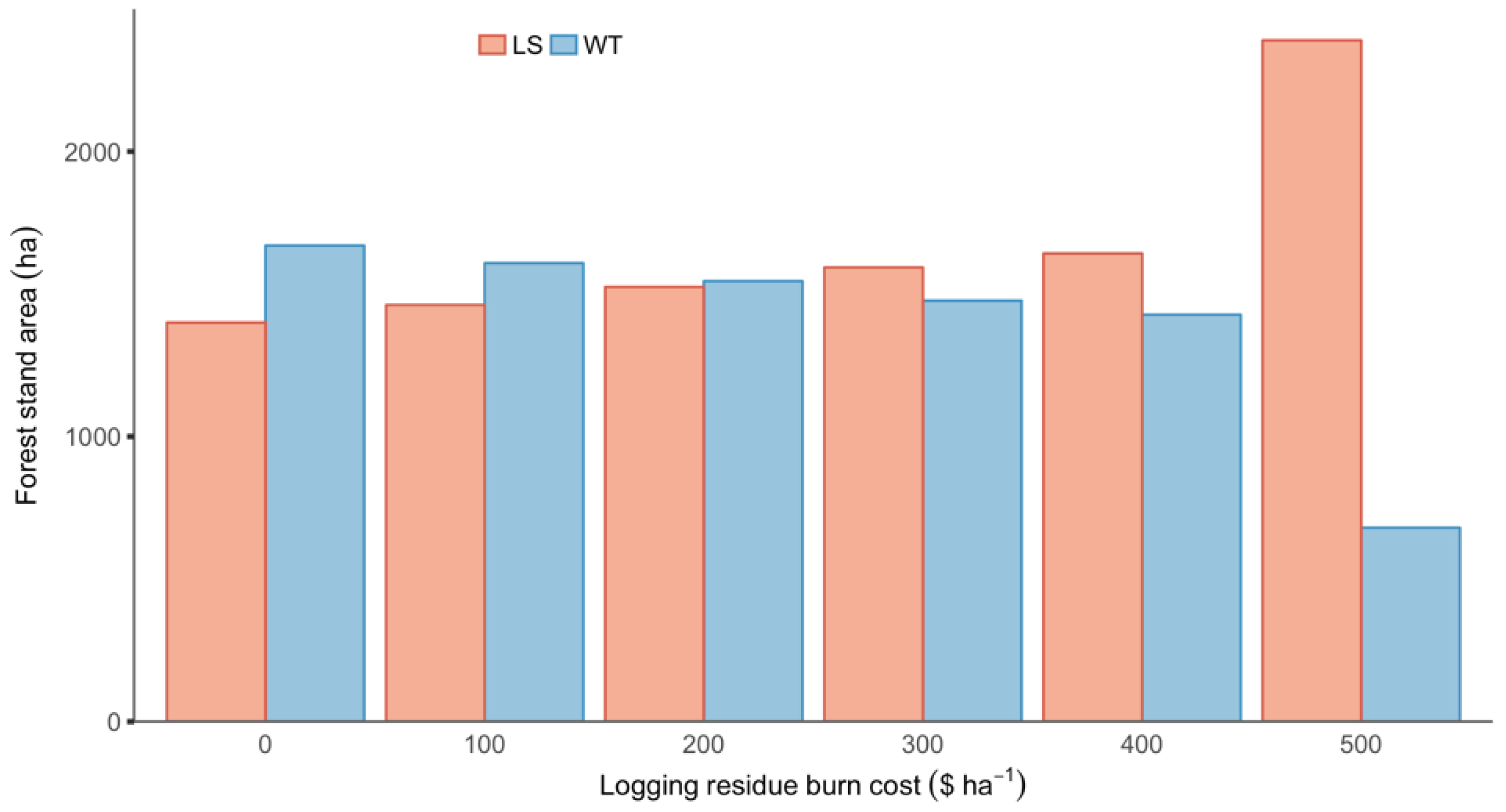
Although WT is a less expensive harvesting method than LS in some areas, producing logging residue piles at the landing may not be ideal if their utilization is not an option due to the lack of biomass markets or high cost downstream logistics (e.g., transportation and storage) that exceed the value of potential biomass feedstock for end users (i.e., gate cost exceeds price). Under such circumstances, additional costs would be incurred for slash pile disposal, typically by open burning, after the WT harvesting is carried out. As a result, the LS system could be a more economically favorable harvesting method than WT in some areas when additional slash pile disposal costs are considered (Figure 7). Indeed, avoidance of slash disposal costs is a major benefit of LS if dispersal of slash on the unit is allowed and lack of biomass markets would necessitate pile burning for slash accumulated on the landing. In the lodgepole pine stands of the Colorado State Forest State Park, based on the results of this analysis, LS and WT would be assigned to almost an equal area when slash disposal costs are about $200 ha⁻¹. When the additional disposal costs become $500 ha⁻¹, there appears to be a significant drop in areas assigned to WT.

Biomass retention may have positive effects on nutrient cycling and long-term site productivity [12,37,38]. The ability to retain biomass on harvest sites for ecological rather than economic reasons is another advantage of LS that was not considered in our cost analysis. However, our estimates on biomass retention after WT show that over 50% of logging residues may be left on the harvest site even if the intention is to remove entire trees. Anecdotal evidence in our study harvest unit, as well as a recent study conducted in the same region [39], show that a large amount of woody debris remains after whole-tree salvage harvest. This can be attributed to the facts that over time limbs and needles naturally fall after trees die and dead trees are more prone to breakage during harvesting operations than live trees. If salvage is conducted during or soon after infestation, while trees are still green, we would expect less leakage during harvest and less biomass retained on site after WT. However, further investigation should be conducted to determine if the amount of biomass retention after WT is sufficient for long-term environmental sustainability, and how retention can change as a result of the timing of harvest.

Potential soil disturbance caused by in-woods operations of heavy machines is another concern regarding long-term site productivity. Compared to WT, LS requires more machines (i.e., delimbers) to operate in the unit, which may cause larger negative impacts on soil, especially when soil is in a fragile condition. Future study should also examine the potential soil impacts of the two harvesting methods to ensure environmental sustainability while meeting the needs of beetle-kill salvage harvest.

5. Conclusions

Our detailed time study of beetle-kill salvage in northern Colorado characterized two commonly used salvage harvest methods in the region in terms of the performance of harvesting systems and individual machines. Our results suggest the following: (1) downed trees significantly and negatively affect feller‒buncher productivity; (2) the efficiency of the delimber more significantly affects the productivity of lop and scatter harvesting; and (3) the productivity of whole-tree harvesting is more sensitive to skidding distance than lop and scatter. Despite some limitations due to the range of variability of the observed operations, such as skidding distance, for example, it is also clear that the application of a single system, regardless of stand conditions and site characteristics, may not be as economically efficient as considering an optimal mix of the two systems across the landscape.

Logging residues are often perceived as a “free” source of biomass at the landing because they are the necessary byproduct of harvesting using whole-tree systems, but our study highlights the fact that there may be actual costs of logging residue production incurred with whole-tree harvesting in the areas where alternatives, such as lop and scatter, exist and are more economical under certain conditions. These additional marginal costs to the landowner should be accounted for along with slash disposal costs and other possible non-market environmental costs when the potential utilization of logging residues is evaluated. Our study implies that the longer the salvage harvest decision and harvest operations are delayed, the greater impact the delay will have on both harvesting costs and the recoverable amount of logging residues (tops, limbs and foliage). However, the non-merchantable amount of bole wood that can be utilized as biomass feedstock would also likely increase over time due to increasing defects on dead trees and the logs produced from them. There is also a tradeoff between biomass recovery and on-site retention from leakage as these stands age. Future research is warranted to address dynamic changes in the quantity and quality of products over time, including biomass recovery, and the financial implications of harvest timing, especially delayed harvesting.

References

- Duda, J.; Lockwood, R.; Mason, L.; Matthews, S.; Mueller, K.; West, D.; Ciesla, W.M. 2015 Report on the Health of Colorado’s Forests: 15 Years of Change; Colorado State Forest Service: Fort Collins, CO, USA, 2016; p. 26. [Google Scholar]
- Anderson, N.; Mitchell, D. Forest operations and woody biomass logistics to improve efficiency, value, and sustainability. Bioenergy Res. 2016, 9, 518–533. [Google Scholar] [CrossRef]
- Nicholls, D.L.; Halbrook, J.M.; Benedum, M.E.; Han, H.-S.; Lowell, E.C.; Becker, D.R.; Barbour, R.J. Socioeconomic Constraints to Biomass Removal from Forest Lands for Fire Risk Reduction in the Western U.S. Forests 2018, 9, 264. [Google Scholar] [CrossRef]
- Yemshanov, D.; McKenney, D.W.; Fraleigh, S.; McConkey, B.; Huffman, T.; Smith, S. Cost estimates of post harvest forest biomass supply for Canada. Biomass Bioenergy 2014, 69, 80–94. [Google Scholar] [CrossRef]
- Zamora-Cristales, R.; Sessions, J.; Boston, K.; Murphy, G. Economic optimization of forest biomass processing and transport in the Pacific Northwest USA. For. Sci. 2015, 61, 220–234. [Google Scholar] [CrossRef]
- Anderson, N.; Chung, W.; Loeffler, D.; Jones, G. A productivity and cost comparison of two systems for producing biomass fuel from roadside forest treatment residues. For. Prod. J. 2012, 62, 222–233. [Google Scholar]
- Han, H.; Chung, W.; Wells, L.; Anderson, N. Optimizing Biomass Feedstock Logistics for Forest Residue Processing and Transportation on a Tree-shaped Road Network. Forests 2018, 9, 121. [Google Scholar] [CrossRef]
- Shabani, N.; Sowlati, T.; Ouhimmou, M.; Rönnqvist, M. Tactical supply chain planning for a forest biomass power plant under supply uncertainty. Energy 2014, 78, 346–355. [Google Scholar] [CrossRef]
- Cambero, C.; Sowlati, T.; Marinescu, M.; Röser, D. Strategic optimization of forest residues to bioenergy and biofuel supply chain. Int. J. Energy Res. 2015, 39, 439–452. [Google Scholar] [CrossRef]
- Bisson, J.; Han, H.-S. Quality of feedstock produced from sorted forest residues. Am. J. Biomass Bioenergy 2016, 5, 81–97. [Google Scholar] [CrossRef]
- Woo, H.; Han, H.-S. Performance of screening biomass feedstocks using star and deck screen machines. Appl. Eng. Agric. 2017, 34, 35–42. [Google Scholar] [CrossRef]
- Matonis, M.; Hubbard, R.; Gebert, K.; Hahn, B.; Miller, S.; Regan, C. Future forests webinar series, webinar proceedings and summary: Ongoing research and management responses to the mountain pine beetle outbreak. In Proceedings of the RMRS-P-70; USDA For. Serv.: Fort Collins, CO, USA, 2014; p. 80. [Google Scholar]
- Lowe, K. Treating Slash after Restoration Thinning; Working Paper; Northern Arizona Univ.: Flagstaff, AZ, USA, 2005. [Google Scholar]
- Weatherspoon, C.P. Residue management in the eastside pine type. In Management of the eastside pine type in northeastern California, proceedings of a symposium, Susanville, CA, USA, 15–17 June 1982; Robson, T.F., Standiford, R.B., Eds.; Northern California Society of American Foresters: Arcata, CA, USA, 1982; pp. 114–121. [Google Scholar]
- Han, H.-S.; Lee, H.W.; Johnson, L.R. Economic feasibility of an integrated harvesting system for small-diameter trees in southwest Idaho. For. Prod. J. 2004, 54, 21–27. [Google Scholar]
- Adebayo, A.B.; Han, H.-S.; Johnson, L. Productivity and cost of cut-to-length and whole-tree harvesting in a mixed-conifer stand. For. Prod. J. 2007, 57, 59–69. [Google Scholar]
- Brinker, R.; Kinard, J.; Rummer, B.; Lanford, B. Machine Rates for Selected Forest Harvesting Machines; Circular 296 (revised); Alabama Agric. Expt. Sta., Auburn Univ.: Auburn, AL, USA, 2002; p. 32. [Google Scholar]
- Olsen, E.; Hossain, M.; Miller, M. Statistical Comparison of Methods Used in Harvesting Work Studies; Research Contribution 23; Forest Research Laboratory, College of Forestry, Oregon State Univ.: Corvallis, OR, USA, 1998; p. 41. [Google Scholar]
- Kim, Y.; Chung, W.; Han, H.; Anderson, N. The effect of downed trees on harvesting productivity and costs in beetle-killed stands. For. Sci. 2017, 63, 596–605. [Google Scholar] [CrossRef]
- R Development Core Team. R: A Language and Environment for Statistical Computing; R Foundation for Statistical Computing: Vienna, Austria, 2014. [Google Scholar]
- Chung, W.; Evangelista, P.; Anderson, N.; Vorster, A.; Han, H.; Krishna, P.; Sturtevant, R. Estimating aboveground tree biomass for beetle-killed lodgepole pine in the Rocky Mountains of northern Colorado. For. Sci. 2017, 63, 413–419. [Google Scholar] [CrossRef]
- Miyata, E.S. Determining fixed and operating costs of logging equipment; Gen. Tech. Rep. NC-55; USDA For. Serv.: Paul, MN, USA, 1980.
- Fight, R.D.; Zhang, X.; Hartsough, B.R. Users Guide for STHARVEST: Software to Estimate the Cost of Harvesting Small Timber; Gen. Tech. Rep. PNW-GTR-582; USDA For. Serv.: Portland, OR, USA, 2003; p. 12.
- Long, J.J.; Boston, K. An evaluation of alternative measurement techniques for estimating the volume of logging residues. For. Sci. 2014, 60, 200–204. [Google Scholar] [CrossRef]
- Hardy, C.C. Guidelines for Estimating Volume, Biomass, and Smoke Production for Piled Slash; Gen. Tech. Rep. PNW-GTR-364; USDA For. Serv.: Portland, OR, USA, 1996; p. 22.
- Wright, C.S.; Balog, C.S.; Kelly, J.W. Estimating Volume, Biomass, and Potential Emissions of Hand-Piled Fuels; Gen. Tech. Rep. PNW-GTR-805; USDA For. Serv.: Portland, OR, USA, 2009; p. 23.
- Pittington Inc. Personal Communication; Pittington Inc.: Walden, CO, USA, 2006. [Google Scholar]
- Nigh, G.; Smith, W. Effects of climate on lodgepole pine stem taper in British Columbia, Canada. Forestry 2012, 85, 579–587. [Google Scholar] [CrossRef]
- Plank, M.E.; Cahill, J.M. Estimating Cubic Volume of Small Diameter Tree-Length Logs From Ponderosa and Lodgepole Pine; Res. Note. PNW-417; USDA For. Serv.: Portland, OR, USA, 1984; p. 7.
- Miles, P.D.; Smith, W.B. Specific Gravity and Other Properties of Wood and Bark for 156 Tree Species Found in North America; Res. Note. NRS-38; USDA For. Serv.: Newtown Square, PA, USA, 2009; p. 35.
- ArcGIS Desktop; Releases 10; ESRI: Redlands, CA, USA, 2012.
- Behjou, F.K.; Majnounian, B.; Namiranian, M.; Dvorak, J. Time study and skidding capacity of the wheeled skidder Timberjack 450c in Caspian forests. J. For. Sci. 2008, 54, 183–188. [Google Scholar] [CrossRef]
- Lotfalian, M.; Moafi, M.; Foumani, B.S.; Akbari, R.A. Time study and skidding capacity of the wheeled skidder Timberjack 450C. Int. J. Sci. Technol. Educ. Res. 2011, 2, 120–124. [Google Scholar]
- Kulak, D.; Stańczykiewicz, A.; Szewczyk, G. Productivity and time consumption of timber extraction with a grapple skidder in selected pine stands. Croat. J. For. Eng. 2017, 38, 55–63. [Google Scholar]
- Twitchell, J.; Gross, R. Personal Communication; Colorado State Forest Service: Walden, CO, USA, 2016. [Google Scholar]
- Mitchell, R.G.; Preisler, H.K. Fall rate of lodgepole pine killed by the mountain pine beetle in central Oregon. West. J. Appl. For. 1998, 13, 23–26. [Google Scholar]
- Rhoades, C.C.; Hubbard, R.M.; Elder, K. A decade of streamwater nitrogen and forest dynamics after a mountain pine beetle outbreak at the Fraser Experimental Forest, Colorado. Ecosystems 2017, 20, 380–392. [Google Scholar] [CrossRef]
- Tinker, D.; Knight, D. Coarse woody debris following fire and logging in Wyoming lodgepole pine forests. Ecosystems 2000, 3, 472–483. [Google Scholar] [CrossRef]
- Hood, P.R.; Nelson, K.N.; Rhoades, C.C.; Tinker, D.B. The effect of salvage logging on surface fuel loads and fuel moisture in beetle-infested lodgepole pine forests. For. Ecol. Manag. 2017, 390, 80–88. [Google Scholar] [CrossRef]
Figure 1.
Site map of the study harvest unit located in the Colorado State Forest State Park.
Figure 2.
Harvesting equipment and operational sequence used in lop and scatter and whole-tree harvesting methods. Harvesting equipment includes feller‒buncher (FB), delimber (DL), skidder (SK), and loader (LO).
Figure 3.
Harvestable lodgepole pine stands in the Colorado State Forest State Park using ground-based equipment shown in diameter at breast height (dbh) classes.
Figure 4.
Economically favorable harvesting methods shown across the lodgepole pine stands in the Colorado State Forest State Park.
Figure 5.
Effects of downed tree proportion on the average harvesting costs and the amount of forest stand areas allocated to the least costly harvesting method between lop and scatter (LS) and whole-tree harvesting (WT).
Figure 6.
Changes in unit production costs over a range of skidding distance estimated for the lop and scatter (LS) and whole-tree harvesting (WT) methods.
Figure 7.
Effects of logging residue disposal costs on economically preferred harvesting method between lop and scatter (LS) and whole-tree harvesting (WT) in the lodgepole pine stands of the Colorado State Forest State Park.