Article

Consequences of a Reduced Number of Plant Functional Types for the Simulation of Forest Productivity

1
Department of Ecological Modelling, Helmholtz Centre for Environmental Research—UFZ, Permoserstr. 15, 04318 Leipzig, Germany
2
Department of Computational Hydrosystems, Helmholtz Centre for Environmental Research—UFZ, Permoserstr. 15, 04318 Leipzig, Germany
3
Institute of Environmental Systems Research, University of Osnabrueck, Barbarastraße 12, 49076 Osnabrueck, Germany
4
German Centre for Integrative Biodiversity Research (iDiv) Halle-Jena-Leipzig, 04103 Leipzig, Germany
*
Author to whom correspondence should be addressed.
Forests 2018, 9(8), 460; https://doi.org/10.3390/f9080460
Submission received: 25 June 2018 / Revised: 20 July 2018 / Accepted: 25 July 2018 / Published: 28 July 2018
(This article belongs to the Special Issue Simulation Modeling of Forest Ecosystems)

Abstract

:
Tropical forests represent an important pool in the global carbon cycle. Their biomass stocks and carbon fluxes are variable in space and time, which is a challenge for accurate measurements. Forest models are therefore used to investigate these complex forest dynamics. The challenge of considering the high species diversity of tropical forests is often addressed by grouping species into plant functional types (PFTs). We investigated how reduced numbers of PFTs affect the prediction of productivity (GPP, NPP) and other carbon fluxes derived from forest simulations. We therefore parameterized a forest gap model for a specific study site with just one PFT (comparable to global vegetation models) on the one hand, and two versions with a higher amount of PFTs, on the other hand. For an old-growth forest, aboveground biomass and basal area can be reproduced very well with all parameterizations. However, the absence of pioneer tree species in the parameterizations with just one PFT leads to a reduction in estimated gross primary production by 60% and an increase of estimated net ecosystem exchange by 50%. These findings may have consequences for productivity estimates of forests at regional and continental scales. Models with a reduced number of PFTs are limited in simulating forest succession, in particular regarding the forest growth after disturbances or transient dynamics. We conclude that a higher amount of species groups increases the accuracy of forest succession simulations. We suggest using at a minimum three PFTs with at least one species group representing pioneer tree species.

1. Introduction

Tropical forests play an important role in the global carbon cycle due to their high productivity and large carbon pools [1,2]. Forests in the tropics are also known for their high species richness with up to 300 tree species per hectare [3,4,5]. Species composition is a driving factor for forest succession, as well as for carbon dynamics. Simulation models are useful tools to investigate these forest dynamics at different scales [6]; for example, global vegetation models provide estimates of forest productivity and carbon budgets at large scales as a function of climate [7,8,9,10,11].
However, including the high species richness in forest models increases enormously the effort for model parameterization and increases uncertainty in model predictions (due to the lack of empirical data for rare tropical tree species). Therefore, it is useful to classify the tree species into a few groups. Several field studies showed that species often show similar attributes (e.g., growth rates), making it possible to group tree species with similar characteristics into species groups known as plant functional types (PFTs) [12,13,14,15]. Species grouping offers a powerful concept that has become relevant for integrating field data in forest models (in the form of parameter values) and comparing simulation results with measurements [16]. With a small number of PFTs, it is easier to interpret the model results, but accuracy improves with an increasing number of PFTs [17].
Especially for dynamic global vegetation models (DGVM)—so far limited to a few PFTs—it is challenging to include a higher number of PFTs due to their global applicability [18,19]. For example, LPJ or SEIB–DGVM normally include only one or two PFTs for tropical regions (tropical broad-leaved evergreen and deciduous trees) [11,20] while a small number of vegetation models [21,22] and some local individual-based forest simulation models often incorporate a higher number of species groups [23]. For local forest models, it has been shown that species grouping allows a realistic description of species dynamics in forests [24]. In particular, forest gap models, such as FORMIND, are able to analyze forest structure and productivity by including up to 20 PFTs [17,25,26].
The creation of functional groups is flexible enough to include relevant trait differences and to avoid functional redundancy between species [17]. Still, it is an open question how many PFTs are appropriate to describe forest dynamics. A low number of PFTs is anyhow of interest in order to reduce the parameterization effort. In this study, we focus on the two following questions:
  • How does the number of PFTs in forest models affect the predictions of aboveground biomass, basal area, forest productivity (GPP, NPP) and carbon sequestration (NEE)?
  • What is the influence of pioneer species on the simulation of forest productivity during the early successional phase in tropical forests?
To address these questions, the individual-based forest gap model FORMIND was applied to a tropical forest site in the Kilimanjaro region of Africa with a single-PFT version (1 PFT), standard-PFT version (3 PFT) and a multi-PFT version (6 PFT). We hypothesize that species diversity, as considered in forest models, significantly influences productivity and carbon flux estimates of forests.

2. Materials and Methods

2.1. Study Site

The tropical submontane forest area, examined in this study, is located within the forest belt at the base of Mt. Kilimanjaro (S3.260150°, E37.417458°). It is located in a steep valley and is largely undisturbed by humans due to restricted accessibility. In this area, five different forest research sites were established with a total size of two hectares. Forest inventories have been conducted in 2012 [27] by the German Research Foundation (DFG) within the Research Unit FOR1246 in cooperation with the Kilimanjaro National Park (FLM forest plots). Stem diameter, tree height, crown expansion, and species identity were determined for every tree with a stem diameter at breast height >10 cm [28,29]. The dataset of one forest stand (forest plot FLM3) represents a forest in equilibrium as it is dominated by late succession species while the fraction of pioneer trees is less than 5%. This study site is dominated by Heinsenia diervilleoides (36% of all trees) and Strombosia scheffleri (24%), Entandophrangma excelsum (6%) and Garcinia tansaniensis (5%)—all shade tolerant tree species. In total, 34 tree species were identified. The investigated forest site has a basal area of 40 m2 ha−1 and it stores approximately 390 tones aboveground biomass per hectare [30]. Aboveground biomass of the field inventory was calculated by summing up the biomass of individual trees using the same allometric relationships as used in the FORMIND model [31].

2.2. Overview of the FORMIND Forest Model

For this study, we used a forest gap model [32], namely the established FORMIND model [25], an individual- and process-based simulation model that was particularly designed for tropical forests. This model has been used for simulating the complex size structure of a forest tree community at a local scale (several hectares). FORMIND includes four main processes: growth of single trees, establishment of new trees, mortality, and competition for light and space. The growth of a single tree is calculated from a carbon balance that includes as main processes photosynthesis, respiration and biomass allocation. Photosynthetic production of an individual tree depends mainly on its light availability (additional limitations can occur due to drought events). FORMIND simulates also above- and belowground carbon stocks and the important carbon fluxes between these stocks. The previous study by Fischer et al. [30] has already shown that Formind can reproduce the essential structural properties of the investigated forest site and also provides realistic values for carbon fluxes. In another study, we proved already that FORMIND is in general able to simulate realistic carbon fluxes by comparing them with eddy covariance data [33]. A detailed description of the FORMIND model can be found in Fischer et al. [25]. This study is based on a parameterization by Fischer et al. [30], determined on the basis of measurements and inventories of a rainforest at Mt. Kilimanjaro. Parameter values used for this study can be found in Appendix A.

2.3. Species Grouping into Plant Functional Types

Tree species were grouped according to their maximum height and light demands (Table 1). Three height classes (<16 m, 16–33 m, >33 m) and three light-requirement classes (shade-tolerant climax species, shade-intolerant pioneer species, and intermediate shade-tolerant species) were used. This resulted in six classes of which each represents one plant functional type, which are already published in [30].

2.4. Model Parameterization Versions

In this study we used three parameterizations with different numbers of PFTs that were applied to the same forest site: a parameterization including only one species (one PFT) with averaged physiological attributes (M1), a standard parameterization with three PFTs representing different light demands (M3), and the parameterization with six PFTs (M6) representing different light demands and height classes (Table 2).
M6 uses exactly the same parameter values as described in Fischer et al. [30]. M1 with only one single PFT is constructed from M6 by averaging the parameters, including weighting factors based on the biomass fraction of each PFT in the forest inventory (for biomass fraction, see Table 1). The same approach was used in M3 for which we grouped species only according to their light demands. The derived model parameter values for the different versions (M1, M3, M6) can be found in Table 3 (overview) and in Appendix A (full list). The calculation of the weights for averaging the parameter values showed that M1 is dominated mainly by shade-tolerant trees as 88% of the biomass belongs to shade tolerant species (Table 1). M3 and M6 include a mixture of shade-tolerant tree species, pioneer species and intermediate shade-tolerant species.

2.5. Simulation Experiments

Starting from bare ground conditions (e.g., after forest disturbances), forest succession was simulated for all parameterization versions on nine hectares over 300 years. We analyzed the aboveground biomass, basal area, mortality, gross primary production, and the net ecosystem exchange (NEE) for the simulated forest stand. These variables were evaluated over the whole simulation time and separately only for the late-successional phase (climax state). For the analyses of the late-successional phase, we averaged the simulation results between the years 200 and 300.

3. Results

Dynamics of a tropical forest were simulated with three different parameterization versions differing in functional diversity from one to six species groups: one PFT (M1), three PFTs (M3) and six PFTs (M6).

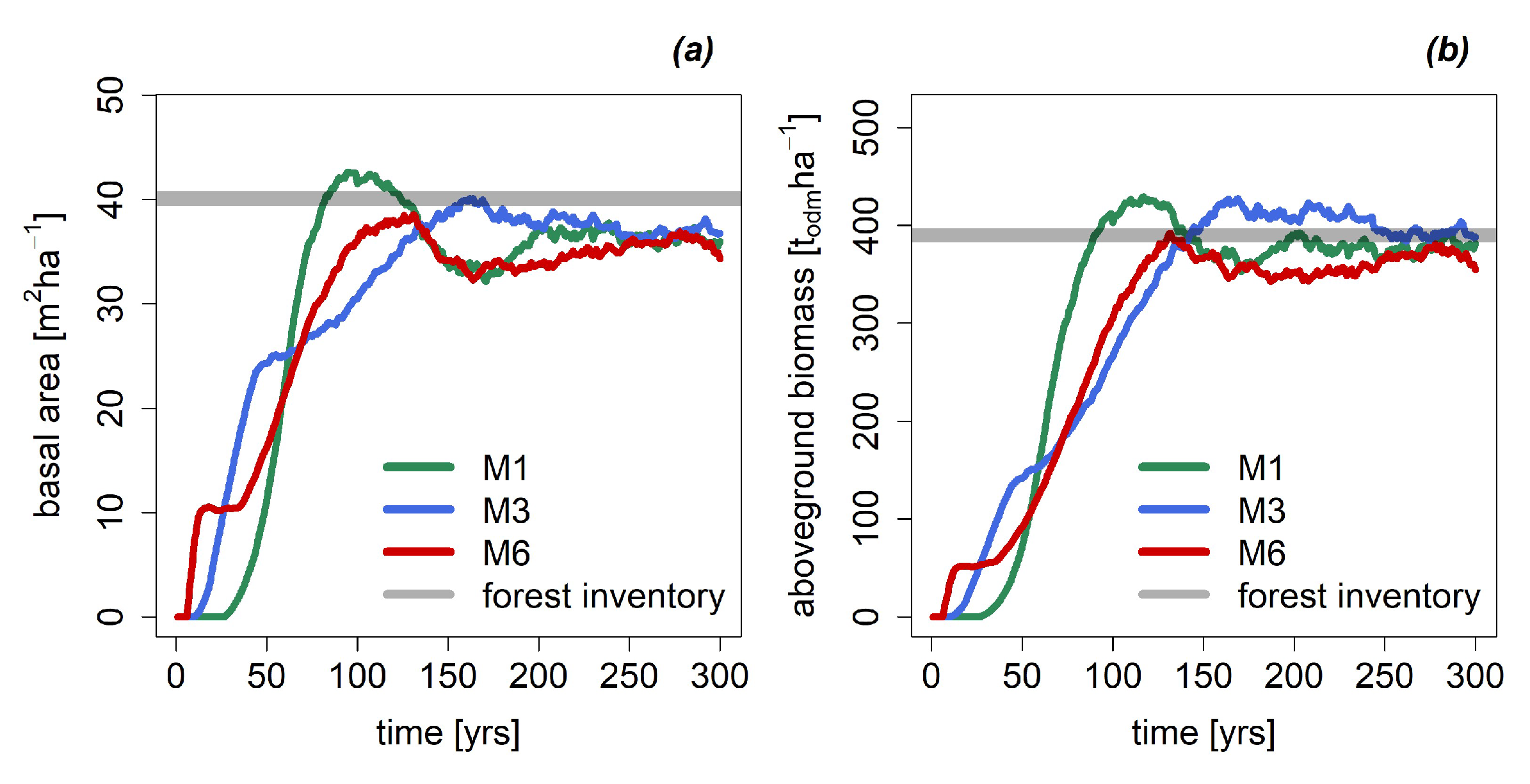
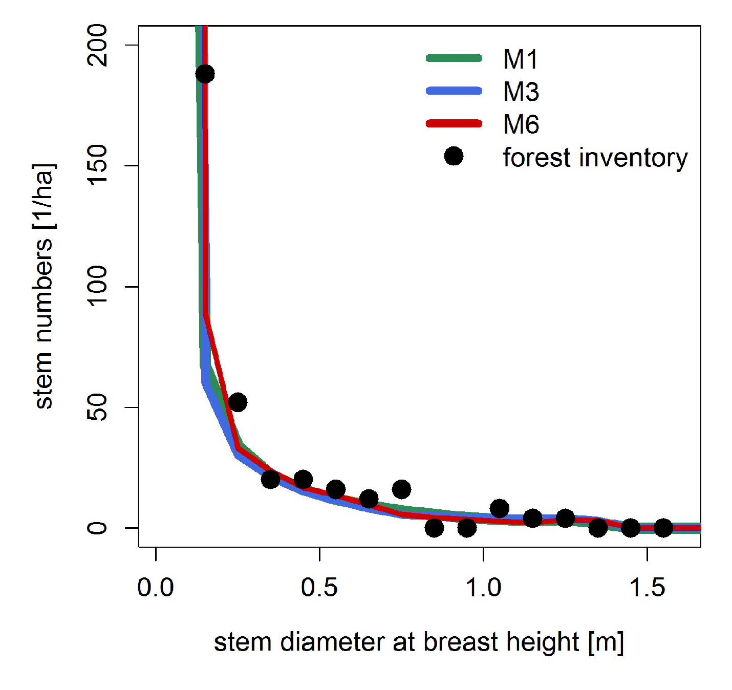
3.1. Basal Area and Biomass

For forests in the late successional-phase, the obtained basal area are nearly equivalent for all of the three parameterization versions (M1: 36.5 m2 ha−1, M3: 37.2 m2 ha−1, M6: 35.3 m2 ha−1; Figure 1a and Table 4) and match nearly the value observed in the field data (40 m2 ha−1). However, the forest in M1 reaches this level of basal area 50 years earlier than the forest in M6 and M3. A similar trend was obtained for aboveground biomass (Figure 1b, Table 4, Figure A1). All simulated forests reach the same level of aboveground biomass in the late-successional phase (360–400 t ha−1), which is comparable to the observed field data (390 t ha−1). Again, M6 and M3 required 50 years more to reach this biomass level. Forest succession is predicted to be slower in the parameterization versions with higher functional diversity (M3, M6). In late successional phase, the simulated stem size distribution matches well the distribution observed in the field (Figure A6).

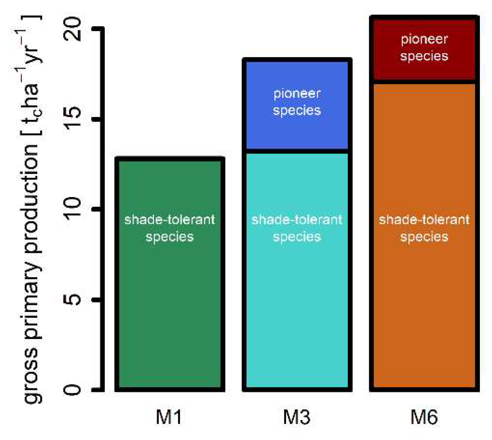
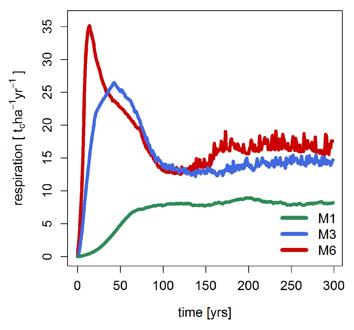
3.2. Mortality, Productivity and Respiration

Biomass loss due to mortality is different for the three simulated forests (Figure 2a, Table 4). For M1, biomass mortality is 15% higher in the late-successional phase than for M6 and 10% higher than for M3. Simulations with M6 included species groups with different light demands and also pioneer trees that often show higher rates of mortality but store less biomass. For M6, a tree has on average 15%–20% less biomass than in M1 (c.f., Figure A3). Biomass loss due to mortality is thus lower in M6 than in M1. This also explains the differences in biomass mortality during the early succession (0–50 years): for M3 and M6, biomass mortality values are 1 tc ha−1 year−1 and 2 tc ha−1 year−1, respectively. For M1, biomass mortality did not occur during the first 50 years (Figure 2a).
Biomass loss due to tree mortality in late-successional phase varies over time, but standard deviation is comparable in all of the parameterization versions, which is mainly caused by mortality events of large trees that occur in all three versions simultaneously (M1: ±1.6 tc ha−1year−1, M3: ±1.4 tc ha−1 year−1, M6: ±1.3 tc ha−1 year−1).
Gross primary productivity (GPP) estimates divergence for the different model parameterization versions (Figure 2b, Table 4). M6 shows 60% higher GPP values than M1 and M3 shows 42% higher GPP values than M1 during the late-successional phase. However, all forest simulations require approximately the same time (~150 years) to reach equilibrium phase. In addition, the variation (standard deviation over time) of GPP was three times larger in M6 than in M1, in M3 two times larger (Figure 2b). Differences are mainly caused by fast-growing and highly productive pioneer tree species that are missing in M1 (c.f., parameter Pmax in Table 3). These pioneer tree species are responsible for one-fifth of the GPP in M6 and one-third in M3 (Figure 3). Surprisingly, GPP of shade-tolerant species in M6 is 30% higher than in M1 and M3 (Figure 3 and Figure A4).
Although we see larger differences in GPP (Figure 2b) and respiration (Figure A2) for the three parameterization versions, there are only minor differences for the net primary productivity (NPP) values, especially in the late-successional phase (Figure 2c, Table 4). We detect 20% more NPP in the late-successional phase in M1 and 5% more in M3 compared to M6. In addition, the fluctuation of NPP in the late-successional phase was highest in M1 (SD in M1 = 0.3 tc ha−1 year−1, M3 = 0.1 tc ha−1 year−1, M6 = 0.1 tc ha−1 year−1).

3.3. Carbon Stocks and Carbon Fluxes

FORMIND simulates above- and belowground carbon stocks, and the total carbon balance of a forest, referred to as net ecosystem exchange (NEE, positive values indicate a carbon sink). All carbon stocks for the mature forest (including aboveground carbon, deadwood pool and soil pool) have value in all parameterization versions (Figure 4a–c). However, the accumulation time until equilibrium differs. While the deadwood and soil pools need 150 years to reach equilibrium in M6 and M3 (Figure 4b,c), these pools are empty for M1 within the first 50 years and then rapidly increase to the equilibrium phase within the next 50 years (Figure 4a). Please note that the dynamics of the deadwood and soil pools are closely related to mortality events of the forest, which are rare within the first 50 years for M1 (c.f., Figure 2a).
NEE was estimated for all parameterization versions (Figure 4d–f). We observe strong differences during the regeneration phase (first 100 years of simulation) with a flux of up to 6 tc ha−1 year−1 for M1 and up to 3 tc ha−1 year−1 in M3 and M6. However, the time span of positive NEE values in M1 and M3 is twice as long as in M1. The strong carbon sink in M1 at the beginning of forest succession (Figure 4d) is caused by the growth of large shade-tolerant trees whereas smaller pioneer trees and trees with intermediate light demands dominate in M3 and M6 (c.f., Figure A1). Pioneer trees have a higher mortality rate and compete with other tree species, which leads to a reduction of NEE values in M3 and M6. After 50 years of succession, more and more large shade-tolerant species colonize the forest and replace the population of pioneer trees for M3 and M6 (Figure A1). This leads to a second peak of NEE during the regeneration phase after 100 years (Figure 4e,f).
Mean NEE in the late-successional phase (200–300 years) is close to zero for all parameterization versions (Figure 4d–f). For M3 and M6, the simulated forests reach this late-successional phase after 150 years, whereas it takes only 100 years in M1. In this phase, carbon fluxes and turnover rates (like productivity and mortality, Figure 2) are relatively constant for all versions, which indicates a stable carbon balance. However, NEE variation (Figure 4d–f) is slightly higher in M1 (+20%), which is a result of larger biomass losses, and therefore larger changes in aboveground biomass and deadwood pool (c.f., Figure 2a).

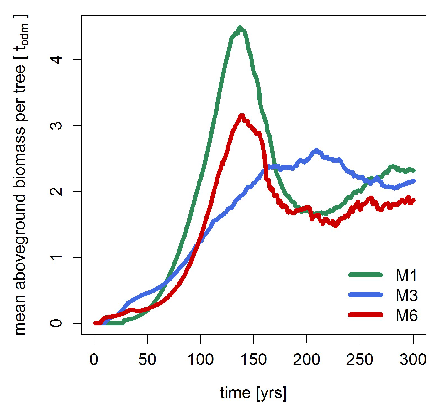
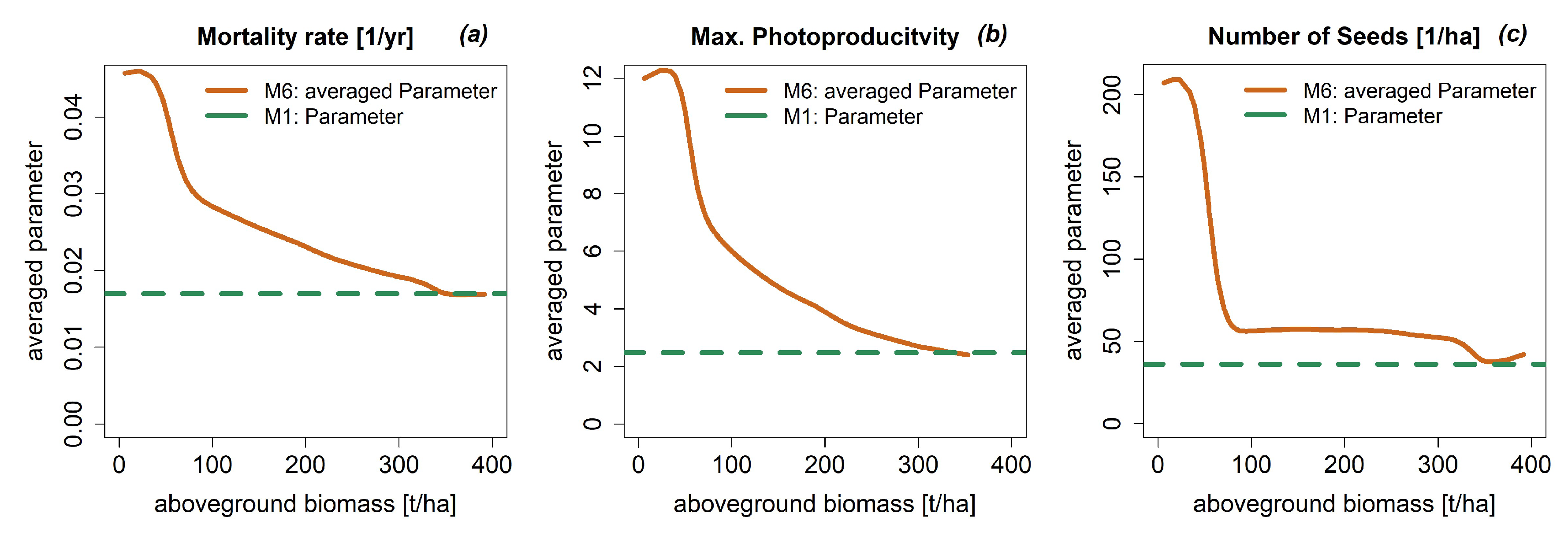
3.4. Dynamic Model Parameters

The parameter values for the processes mortality, photosynthesis and recruitment of M1 were compared with a dynamically averaged parameter of M6. Dynamically averaged parameters of M6 are calculated for each time step by averaging the six different parameter values for each PFT, weighted by the current simulated biomass fraction for each PFT. In the early successional phase, the forest is dominated by pioneer species, so the averaged parameter value for M6 is comparable to the parameter values of pioneer species. Therefore, it is evident that the averaged parameter of M6 differs significantly from M1 (Figure 5), especially before the early-successional phase (<100 years). Mean mortality rate of M6 is twice as high in this phase, maximum photoproductivity almost four times as high and number of seeds five times higher compared to M1 (Figure 5). From the mid-successional phase onwards (>100 years), the dynamically averaged parameters of M6 are similar to the values of M1. In this phase, the forest is dominated by climax species, which is comparable to the parameter values of the climax species, which resulted in a very similar parameter value of M1 and averaged parameter of M6.

4. Discussion

4.1. The Influence of Species Grouping on Forest Dynamic Simulations

In this study, we evaluated the role of species grouping for forest modeling and analyzed the impact of a reduced number of species groups on forest productivity and carbon flux estimations. Using an established forest model, we simulated the dynamics of an African tropical forest with three different model parameterization versions differing in the number of plant functional types (PFT): M1 includes only one PFT and is based on the assumption that all trees are similar in their physiological attributes (mean species approach). This resulted in one species group with averaged attributes—an approach that is comparable to those made in global vegetation models [e.g. SEIB–DGVM 11, and LPJ 20]. The advantage of such a mean-species approach is that it reduces parameterization effort and model runtime (c.f., Table 4).
We showed that reducing the number of PFTs to only one species type has a strong influence on derived vegetation dynamics. This approach simulates only intraspecific competition between trees and hence rather corresponds to a monoculture. Moreover, we could show that the pronounced heterogeneity in forest structure prevalent in tropical forests (e.g., different height layers) could not be reproduced with one mean-species. The approach using one PFT has a reduced realism because of its constant parameter value, which does not allow for the adaptation to the environment or niches [34]. However, a parameterization with one species group is sufficient to derive reasonable values for biomass, basal area, and NEE of mature forests, whereas the species grouping plays an important role in earlier successional phases.
Estimates of forest productivity, on the other hand, are highly sensitive to the number of included PFTs. The absence of pioneer tree species in the species grouping (M1) leads to a decrease of gross primary production by 60% (compared to M6) and a 50% increase of carbon sinks (NEE). These findings may have a strong impact on productivity estimates at regional and continental scales [10,20,35]. Although our study was conducted for one study site, the pattern of our results seems to be generally valid and transferable to other locations due to the structural realism of the gap model (individual-based and process-based). In fact, our results, that young pioneer-dominated tropical forests are more productive than old-growth forests, are in close agreement with a field-inventory based study across the Amazon basin [36].
A basic assumption for many models with PFT grouping is that the parameter values (e.g., for growth or mortality) always remain constant for the respective PFT—independent of the species composition within the PFT. This can be a disadvantage when describing a forest by just a single shade-tolerant PFT. As in M1, the representation of pioneer species is missing. An alternative approach to include functional diversity into forest models with just one PFT can be the approach of dynamic model parameters, which change their parameter value depending on the successional state of the simulated forest. For example, an early stage forest could have a higher mortality rate than a mature forest (due to a shift in species composition). Thus, the mortality parameter of a PFT could be adjusted according to the successional state of the forest (c.f., Figure 5). However, it is difficult to determine the successional age of a forest (especially with only one PFT), which is why we suggest to relate the dynamic model parameter value to a measurable forest variable like forest biomass (Figure A5). A dynamic parameterization could then imitate different species compositions even in models with a small number of PFTs, and thus represent the succession in the forest more accurately.

4.2. Functional Diversity and Forest Structure in DGVMs

Dynamic global vegetation models (DGVMs) are valuable tools for estimating forest productivity and carbon budgets at the large scale [37]. Traditional DGVMs simulate vegetation dynamics with a resolution of 50 kilometers and are not able to represent forest structure, individual trees, and high species diversity. With a few exceptions, such as ED2 [22], most DGVMs use only one shade-tolerant PFT per biome for the simulations of tropical forests [11,20]. Consequently, it is challenging to reproduce forest successions with these models, as competition between trees is only partly represented. In this study, we showed that this can lead to a relevant bias in forest productivity estimates.
Local forest models have the ability to include functional diversity and structural realism due to their individual- and process-based approach. Such models are capable of providing reliable estimates of forest dynamics [25,33]. This advantage has been recognized and the concept of forest gap models has been tried to incorporate within the DGVM framework, such as the SEIB-DGVM [11], LPJ-GUESS [38], and the ORCHIDEE-CAN model [39]. This means that gap dynamics are included, but species diversity is still only defined by one or two PFTs per biome depending on climatic conditions [40].
A novel strategy is to include functional diversity in vegetation models by using trait distributions [41]. This is a promising approach for large-scale vegetation modeling. However, please note that the trade-offs between traits of tropical tree species are challenging to estimate. Enhancing databases on plant traits [42] will play a major role for this modeling approach in the future. Another novel approach allows for including more species diversity into large-scale vegetation modeling by applying traditional forest models on entire landscapes or biomes at the individual tree level [43,44]. Such forest models are particular important to investigate forests through all successional states, investigate disturbed forests [45] and show potential in linking simulations with remote sensing [46,47].

4.3. Challenges of the PFT Approach in Forest Models

The categorization into PFTs is often based on inventory data. This is the reason why forest gap models are sometimes blamed to be ‘data-hungry’ [48,49]. However, species grouping is a suitable and efficient approach for dealing with species-rich ecosystems—very often the only option for modeling species diversity at all. Köhler et al. [12] found that modeling studies have used between five and up to 50 PFTs. Finding the right balance between appropriate and necessary accuracy has not yet been treated satisfactorily. The study by Köhler et al. recommends applying a grouping which is based on successional status (three groups) and maximum height (five groups). This classification is in accordance with our finding that species should be grouped by successional status or light demands. However, the concept by Köhler et al. is related with a high parameterization effort—reducing the number of height layers in this case could be a good suggestion. In addition, the assignment of species to a single functional group is sometimes challenging [14] in the case that intra-specific variability of functional traits is higher than the inter-specific variability.
For a single study, it is quite straightforward to define clear grouping criteria (e.g., maximum attainable height of each species) and to implement a categorization (e.g., maximum height between 10 m and 20 m). Grouping strategy depends always on the research question and study site, which means that there can be no general criteria for an appropriate species grouping [14,50]. Therefore, it is challenging to transfer an established PFT classification from one study site to another region [51]. In a recent study [44], a method has been developed on how to transfer a local forest model parameterization across an entire region. In this regionalization approach, environmental conditions have been taken as a proxy for the mortality rate (instead of constant mortality rates for the entire biome), which is normally a site-specific parameter. Thereby, the forest model is able to reproduce spatially variable forest dynamics.
Moreover, different species grouping concepts can be available for the same study region [15]. In the study by Picard et al., five different species groupings were compared for the same tropical forest site. The groupings agreed mainly on tree height classification but differed with respect to light requirements of the trees. Again, various research questions can of course lead to different species grouping even for the same study site.
There are many published species grouping around for different regions in the tropics which can serve as a starting point if a new site-specific grouping is needed. These different groupings should be analyzed and compared in future. It could even turn out that these published groupings may not be so different at all.

5. Conclusions

The number of considered PFTs is a crucial aspect for the accuracy of forest simulations, especially when investigating mortality, productivity and carbon fluxes. Our results show that vegetation models, which are based on the mean-species approach, may predict other carbon fluxes than vegetation models with a higher number of PFTs. Therefore, some model versions may be limited by their predictive capabilities to describe forest growth in transient dynamics. Incorporating more species groups can be an important factor for simulations of forest succession as well as for describing the carbon dynamics of a forest. Pioneer species play a crucial role in the simulation of forest dynamics, especially for research questions related to forest productivity in tropical regions. In order to represent forest succession, we suggest using at least three PFTs in tropical forest modeling—one group of pioneer tree species, one group of shade-tolerant climax species and one group of intermediate shade-tolerant tree species. This is particularly relevant for simulating forest succession after disturbances (e.g., fire, logging, wind throws), climate change, or land use.

Author Contributions

Conceptualization, R.F. and A.H.; Data curation, R.F.; Formal analysis, R.F.; Funding acquisition, A.H.; Methodology, R.F.; Software, R.F., E.R. and A.H.; Validation, R.F.; Visualization, R.F.; Writing—Original draft, R.F., E.R. and A.H.

Funding

This study was conducted within the framework of the research unit FOR1246 (Kilimanjaro ecosystems under global change: linking biodiversity, biotic interactions and biogeochemical ecosystem processes) funded by the Deutsche Forschungsgemeinschaft (DFG). We acknowledge funding from the Helmholtz Alliance “Remote Sensing and Earth System Dynamics”. Andreas Huth was also supported by the European Research Council (ERC) advanced grant 233066.

Acknowledgments

We want to thank Felix May for helpful discussions and constructive comments on the manuscript. We would like to thank the two anonymous reviewers for their helpful suggestions and comments.

Conflicts of Interest

The authors declare that there is no conflict of interest regarding the publication of this article.

Appendix A

FORMIND model description and full parameter list for the parameterization versions M1, M3 and M6. Additional simulation results of the forest dynamics with FORMIND.

Appendix A.1.: Model Description and Parameter Values

FORMIND is an individual-based, spatially explicit and process-based model designed to simulate the dynamics of species-rich forests [25]. The model simulates the processes of establishment, growth, competition and mortality of trees on a regular grid of patches with the dimensions of a typical treefall gap (20 m × 20 m). Within each patch, the trees do not have explicit spatial positions following the gap-model concept (Shugart, 1984). By combining many patches, large forest areas up to hundreds of hectares can be simulated. Tree species with similar ecological traits are aggregated into plant functional types (PFT) to facilitate parameterization for diverse forests and reduce computation time. The PFTs may represent different successional types (from pioneers to climax species) and size classes (from understory to emergent species).
In each simulated time step (1 year), the following main processes take place: (1) Establishment: Seeds are distributed over the forest area. If light conditions are suitable, new saplings can establish and compete for light and space in the patch. (2) Competition: The main driving factor of the model is light. Radiation intensity within each patch decreases from the top to the ground according to a light extinction function. The light extinction depends on the combined vertical leaf area profile of all trees in the patch. The productivity of each tree is determined by the available light in its height layer. (3) The growth of each tree depends on its gross primary productivity (GPP), respiration and PFT-specific physiological and allometric parameters. (4) Mortality: Trees die stochastically according to a PFT-specific mortality rate. If a tree falls, it can damage neighboring trees in adjacent patches. Besides these core processes, FORMIND offers the following feature: Carbon Cycle: Gross primary production, respiration and net primary production are calculated for each individual tree. Based on this, the carbon balance for a whole forest can be derived, including soil respiration and net ecosystem productivity.
The detailed model description was published with Fischer et al. [25]. Parameters for the study site Mt. Kilimanjaro (plot FLM 3), Tanzania are listed in Table A1, Table A2 and Table A3 below. All model parameters are explained in Fischer et al. [25]. The description of all parameters can be found in the handbook; only the parameter values for the current study are specified here. All parameter values for the original parameterization (M6) are already published in Fischer et al. [30]. All parameter values for the parameterization versions with a reduced number of PFTs (M3 and M1) are the result of averaging the parameters of M6.
Table A1. Generic parameters for all three parameterization versions M1, M3 and M6.
ParameterUnitValueReferences
Generaltendyear300technical parameter
tyyear1technical parameter
Aareaha9technical parameter
Apatchm2400technical parameter
MaxGrp 1,3,6technical parameter
Δhm0.5technical parameter
Carbon CycleAETmm year−11300[30]
tSslow -> Ayear−11/750[11]
tSfast -> Ayear−11/15[11]
Photo-synthesisI0μmolphoton m−2 s−1870[30]
k 0.7[30,52]
ldayh12[30]
ϕactd360[30]
Geometrycl0 0.30[30,31,53]
cd0 13.75field data
cd1 0.68field data
σ 0.70[30,31,54]
f0 0.34[30,31]
f1 −0.18[30,31]
l0 3.17[30,31]
l1 0.10[30,31]
Othersffall 0.4[30,55]
Othersrg 0.25[30,56]
Table A2. PFT-specific parameters for M6.
ParameterUnitPlant Functional Type (PFT)Ref.
123456
GeometryHmaxm563333281616field data
h0 45.2830.6636.5630.9320.8247.55field data
h1 0.570.410.440.430.340.6field data
ρtODM/m30.550.540.410.40.520.47field data
RecruitmentNseedha−1 year−130156213002200[30]
Iseed 0.030.010.050.200.030.20[30,57]
Dminm0.02[30]
MortalityMByear−10.0150.030.0290.040.0210.045[30]
Photo-synthesispmaxμmolCO2 μmolphoton−12.03.16.811.07.012.0[30,31,58,59]
αμmolCO2 m−2 s−10.360.280.230.200.300.20[30,31,58,59]
Growth∆D maxm year−10.0120.0120.0190.0290.0110.029[30]
D ∆D max%0.330.340.230.600.330.60[30]
Table A3. PFT-specific parameters for M3 and M1.
ParameterUnitVersion M3Version M1
I (1,2,5)II (3)III (4,6)I (1–6)
GeometryHmaxm55.23327.153.2
h0 44.7936.5632.1444.049
h1 0.560.440.440.554
ρtODM/m30.540.410.410.537
RecruitmentNseedha−1 year−1342129333
Iseed 0.0290.050.200.032
Dminm0.020.02
MortalityMByear−10.01540.0290.04040.017
Photo-synthesispmaxμmolCO2 μmolphoton−12.056.8011.072.479
αμmolCO2 m−2 s−10.3570.2300.2000.346
Growth∆D maxm year−10.0120.0190.0290.013
D ∆D max%0.33030.230.600.323

Appendix A.2.: Simulation of the Forest Dynamics with FORMIND

Figure A1. Visualization of one hectare of simulated tropical forest for Kilimanjaro region with the FORMIND model. Snapshot after 100 years of forest succession: (a) forest simulation with one PFT (averaged species, M1) and (b) with six PFTs (M6, see Table 1). The colors of the crowns represent different plant functional types. In addition, the biomass dynamics for the different parameterization versions (see Table 2) are presented. M1 shows the biomass dynamics for the averaged PFT (c). M3 shows the biomass succession for three PFTs differentiated after light demands (d). M6 shows biomass succession with six PFTs differentiated after height classes and light demands (e). PFT 1, 2 and 5 are climax species (greenish), PFT 3 intermediate shade-tolerant species (blue), and PFT 4 and 6 are pioneer species (red/orange). In the simulation, the fraction of biomass in old-growth state is dominated by PFT 1 (d,e). The biomass of pioneer species is less than 1% in old-growth state (d,e).
Forests 09 00460 g0a1
Figure A2. Simulated total respiration of living biomass (total respiration = maintenance + growth respiration) for the simulated tropical forest. The lower GPP in M1 also leads to a lower respiration rate. In particular, growth respiration in M1 is 35% less than in M6. Growth respiration in M6 differs only slightly with 10% lower values than in M3. Maintenance respiration was similar in all parameterization versions. This seems to be reasonable as maintenance respiration depends mainly on standing biomass, which is also similar in all three versions.
Forests 09 00460 g0a2
Figure A3. Aboveground biomass per tree (total biomass divided by stem numbers) over time for all parameterization versions. Mean biomass per tree is lower in M6 (with six PFTs) compared to M1 (with one PFT). In particular, in late-successional phase, trees have 15%–20% less biomass in M6 compared to M1.
Forests 09 00460 g0a3
Figure A4. Simulated gross primary production (GPP) over time for M1, M3 and M6. For the parameterization versions with more than one PFT (M3 and M6), we subdivided total GPP into GPP of shade tolerant species and pioneer species.
Forests 09 00460 g0a4
Figure A5. Presented are the same parameters of the FORMIND model as in Figure 5, but here as a function of simulated total aboveground biomass instead of simulation time. The main parameters of the FORMIND model: (a) mortality rate, (b) maximum photoproductivity and (c) number of seeds for two different parameterizations (M1 with 1 PFT and M6 with 6 PFTs). The averaging of the parameter for M6 is the same as described in Figure 5. Detailed biomass dynamics of M1 and M6 are shown in Figure A1.
Forests 09 00460 g0a5

Appendix A.3.: Testing Model Simulations with Field Data

For model calibration, we also analyzed tree stem size distributions in late-successional phase (number of trees for different stem diameter classes). The distributions are found to be similar for all three parameterization versions (Figure A6) independent of its number of PFTs. Results match the stem size distribution observed in the field. Smaller differences between simulation and field data occur in the diameter class 20–30 cm (+19 trees/ha) and 70–80 cm (+9 trees/ha).
Figure A6. Simulated stem size distribution for the late-successional phase. Shown are the results from the parameterization versions M1, M3 and M6. Field data from Mt. Kilimanjaro are shown as black dots.
Forests 09 00460 g0a6

References

  1. Bonan, G.B. Forests and climate change: Forcings, feedbacks, and the climate benefits of forests. Science 2008, 320, 1444–1449. [Google Scholar] [CrossRef] [PubMed]
  2. Pan, Y.D.; Birdsey, R.A.; Fang, J.Y.; Houghton, R.; Kauppi, P.E.; Kurz, W.A.; Phillips, O.L.; Shvidenko, A.; Lewis, S.L.; Canadell, J.G.; et al. A large and persistent carbon sink in the world's forests. Science 2011, 333, 988–993. [Google Scholar] [CrossRef] [PubMed]
  3. Pimm, S.L.; Raven, P. Biodiversity - extinction by numbers. Nature 2000, 403, 843–845. [Google Scholar] [CrossRef] [PubMed]
  4. Slik, J.W.F.; Arroyo-Rodríguez, V.; Aiba, S.-I.; Alvarez-Loayza, P.; Alves, L.F.; Ashton, P.; Balvanera, P.; Bastian, M.L.; Bellingham, P.J.; van den Berg, E.; et al. An estimate of the number of tropical tree species. Proc. Natl. Acad. Sci. USA 2015, 112, 7472–7477. [Google Scholar] [CrossRef] [PubMed] [Green Version]
  5. ter Steege, H.; Pitman, N.C.A.; Sabatier, D.; Baraloto, C.; Salomão, R.P.; Guevara, J.E.; Phillips, O.L.; Castilho, C.V.; Magnusson, W.E.; Molino, J.-F.; et al. Hyperdominance in the amazonian tree flora. Science 2013, 342. [Google Scholar] [CrossRef] [PubMed]
  6. Snell, R.S.; Huth, A.; Nabel, J.E.M.S.; Bocedi, G.; Travis, J.M.J.; Gravel, D.; Bugmann, H.; Gutiérrez, A.G.; Hickler, T.; Higgins, S.I.; et al. Using dynamic vegetation models to simulate plant range shifts. Ecography 2014, 37, 1184–1197. [Google Scholar] [CrossRef] [Green Version]
  7. Friend, A.D.; Shugart, H.H.; Running, S.W. A physiology-based model of forest dynamics. Ecology 1993, 74, 792–797. [Google Scholar] [CrossRef]
  8. Rammig, A.; Jupp, T.; Thonicke, K.; Tietjen, B.; Heinke, J.; Ostberg, S.; Lucht, W.; Cramer, W.; Cox, P. Estimating the risk of amazonian forest dieback. New Phytol. 2010, 187, 694–706. [Google Scholar] [CrossRef] [PubMed]
  9. Friend, A.D.; Arneth, A.; Kiang, N.Y.; Lomas, M.; Ogee, J.; Rodenbeckk, C.; Running, S.W.; Santaren, J.D.; Sitch, S.; Viovy, N.; et al. Fluxnet and modelling the global carbon cycle. Glob. Chang. Biol. 2007, 13, 610–633. [Google Scholar] [CrossRef]
  10. Verbeeck, H.; Peylin, P.; Bacour, C.; Bonal, D.; Steppe, K.; Ciais, P. Seasonal patterns of co2 fluxes in amazon forests: Fusion of eddy covariance data and the orchidee model. J. Geophys. Res. Biogeosci. 2011, 116, G02018. [Google Scholar] [CrossRef]
  11. Sato, H.; Itoh, A.; Kohyama, T. Seib-dgvm: A new dynamic global vegetation model using a spatially explicit individual-based approach. Ecol. Model. 2007, 200, 279–307. [Google Scholar] [CrossRef]
  12. Köhler, P.; Ditzer, T.; Huth, A. Concepts for the aggregation of tropical tree species into functional types and the application on sabah's dipterocarp lowland rain forests. J. Trop. Ecol 2000, 16, 591–602. [Google Scholar] [CrossRef]
  13. Smith, T.M.; Shugart, H.H. Plant Funct. Types; Cambridge University Press: Cambridge, UK, 1997. [Google Scholar]
  14. Gourlet-Fleury, S.; Blanc, L.; Picard, N.; Sist, P.; Dick, J.; Nasi, R.; Swaine, M.D.; Forni, E. Grouping species for predicting mixed tropical forest dynamics: Looking for a strategy. Ann. For. Sci. 2005, 62, 785–796. [Google Scholar] [CrossRef]
  15. Picard, N.; Köhler, P.; Mortier, F.; Gourlet-Fleury, S. A comparison of five classifications of species into functional groups in tropical forests of french guiana. Ecol. Complex. 2012, 11, 75–83. [Google Scholar] [CrossRef]
  16. Vanclay, J.K.; Skovsgaard, J.P. Evaluating forest growth models. Ecol. Model. 1997, 98, 1–12. [Google Scholar] [CrossRef] [Green Version]
  17. Kazmierczak, M.; Wiegand, T.; Huth, A. A neutral vs. Non-neutral parametrizations of a physiological forest gap model. Ecol. Model. 2014, 288, 94–102. [Google Scholar] [CrossRef]
  18. Lavorel, S.; D¡az, S.; Cornelissen, J.H.C.; Garnier, E.; Harrison, S.P.; McIntyre, S.; Pausas, J.G.; P‚rez-Harguindeguy, N.; Roumet, C.; Urcelay, C. Plant functional types: Are we getting any closer to the holy grail. In Terrestrial Ecosystems in a Changing World; Canadell, J.G., Pataki, D., Pitelka, L.F., Eds.; Springer: Berlin, Germany, 2007. [Google Scholar]
  19. Poulter, B.; Ciais, P.; Hodson, E.; Lischke, H.; Maignan, F.; Plummer, S.; Zimmermann, N.E. Plant functional type mapping for earth system models. Geosci. Model Dev. 2011, 4, 993–1010. [Google Scholar] [CrossRef] [Green Version]
  20. Sitch, S.; Smith, B.; Prentice, I.C.; Arneth, A.; Bondeau, A.; Cramer, W.; Kaplan, J.O.; Levis, S.; Lucht, W.; Sykes, M.T.; et al. Evaluation of ecosystem dynamics, plant geography and terrestrial carbon cycling in the lpj dynamic global vegetation model. Glob. Chang. Biol. 2003, 9, 161–185. [Google Scholar] [CrossRef]
  21. Medvigy, D.; Wofsy, S.C.; Munger, J.W.; Hollinger, D.Y.; Moorcroft, P.R. Mechanistic scaling of ecosystem function and dynamics in space and time: Ecosystem demography model version 2. J. Geophys. Res. Biogeosci. 2009, 114, G01002. [Google Scholar] [CrossRef]
  22. Kim, Y.; Knox, R.G.; Longo, M.; Medvigy, D.; Hutyra, L.R.; Pyle, E.H.; Wofsy, S.C.; Bras, R.L.; Moorcroft, P.R. Seasonal carbon dynamics and water fluxes in an a mazon rainforest. Glob. Chang. Biol. 2012, 18, 1322–1334. [Google Scholar] [CrossRef]
  23. Shugart, H.H. A Theory of Forest Dynamics; The Blackburn Press: Blackburn Road, Prince George, BC, Canada, 2003. [Google Scholar]
  24. Köhler, P.; Huth, A. The effects of tree species grouping in tropical rainforest modelling: Simulations with the individual-based model formind. Ecol. Model. 1998, 109, 301–321. [Google Scholar] [CrossRef] [Green Version]
  25. Fischer, R.; Bohn, F.; Dantas de Paula, M.; Dislich, C.; Groeneveld, J.; Gutiérrez, A.G.; Kazmierczak, M.; Knapp, N.; Lehmann, S.; Paulick, S.; et al. Lessons learned from applying a forest gap model to understand ecosystem and carbon dynamics of complex tropical forests. Ecol. Model. 2016, 326, 124–133. [Google Scholar] [CrossRef] [Green Version]
  26. Köhler, P.; Huth, A. Simulating growth dynamics in a south-east asian rainforest threatened by recruitment shortage and tree harvesting. Clim. Chang. 2004, 67, 95–117. [Google Scholar]
  27. Peters, M.K.; Hemp, A.; Appelhans, T.; Behler, C.; Classen, A.T.; Detsch, F.; Ensslin, A.; Ferger, S.W.; Frederiksen, S.B.; Gebert, F.; et al. Predictors of elevational biodiversity gradients change from single taxa to the multi-taxa community level. Nat. Commun. 2016, 7, art. 13736. [Google Scholar] [CrossRef] [PubMed]
  28. Rutten, G.; Ensslin, A.; Hemp, A.; Fischer, M. Forest structure and composition of previously selectively logged and non-logged montane forests at mt. Kilimanjaro. For. Ecol. Manag. 2015, 337, 61–66. [Google Scholar] [CrossRef]
  29. Ensslin, A.; Rutten, G.; Pommer, U.; Zimmermann, R.; Hemp, A.; Fischer, M. Effects of elevation and land use on the biomass of trees, shrubs and herbs at mount kilimanjaro. Ecosphere 2015, 6, 1–15. [Google Scholar] [CrossRef]
  30. Fischer, R.; Ensslin, A.; Rutten, G.; Fischer, M.; Schellenberger Costa, D.; Kleyer, M.; Hemp, A.; Paulick, S.; Huth, A. Simulating carbon stocks and fluxes of an african tropical montane forest with an individual-based forest model. PLoS ONE 2015, 10, e0123300. [Google Scholar] [CrossRef] [PubMed] [Green Version]
  31. Dislich, C.; Günter, S.; Homeier, J.; Schröder, B.; Huth, A. Simulating forest dynamics of a tropical montane forest in south ecuador. Erdkunde 2009, 63, 347–364. [Google Scholar] [CrossRef]
  32. Shugart, H.H.; Wang, B.; Fischer, R.; Ma, J.; Fang, J.; Yan, X.; Huth, A.; Armstrong, A.H. Gap models and their individual-based relatives in the assessment of the consequences of global change. Environ. Res. Lett. 2018, 13, 033001. [Google Scholar] [CrossRef] [Green Version]
  33. Rödig, E.; Huth, A.; Bohn, F.; Rebmann, C.; Cuntz, M. Estimating the carbon fluxes of forests with an individual-based forest model. For. Ecosyst. 2017, 4. [Google Scholar]
  34. Van Bodegom, P.M.; Douma, J.C.; Witte, J.P.M.; Ordoñez, J.C.; Bartholomeus, R.P.; Aerts, R. Going beyond limitations of plant functional types when predicting global ecosystem–atmosphere fluxes: Exploring the merits of traits-based approaches. Glob. Ecol. Biogeogr. 2012, 21, 625–636. [Google Scholar] [CrossRef]
  35. Poulter, B.; Aragão, L.; Heyder, U.; Gumpenberger, M.; Heinke, J.; Langerwisch, F.; Rammig, A.; Thonicke, K.; Cramer, W. Net biome production of the amazon basin in the 21st century. Glob. Chang. Biol. 2010, 16, 2062–2075. [Google Scholar] [CrossRef]
  36. Poorter, L.; Bongers, F.; Aide, T.M.; Zambrano, A.M.A.; Balvanera, P.; Becknell, J.M.; Boukili, V.; Brancalion, P.H.; Broadbent, E.N.; Chazdon, R.L. Biomass resilience of neotropical secondary forests. Nature 2016, 530, 211–214. [Google Scholar] [CrossRef] [PubMed]
  37. Le Quéré, C.; Andrew, R.M.; Canadell, J.G.; Sitch, S.; Korsbakken, J.I.; Peters, G.P.; Manning, A.C.; Boden, T.A.; Tans, P.P.; Houghton, R.A.; et al. Global carbon budget 2016. Earth Syst. Sci. Data 2016, 8, 605–649. [Google Scholar] [CrossRef]
  38. Hickler, T.; Vohland, K.; Feehan, J.; Miller, P.A.; Smith, B.; Costa, L.; Giesecke, T.; Fronzek, S.; Carter, T.R.; Cramer, W.; et al. Projecting the future distribution of european potential natural vegetation zones with a generalized, tree species-based dynamic vegetation model. Glob. Ecol. Biogeogr. 2012, 21, 50–63. [Google Scholar] [CrossRef]
  39. Naudts, K.; Ryder, J.; McGrath, M.J.; Otto, J.; Chen, Y.; Valade, A.; Bellasen, V.; Berhongaray, G.; Bönisch, G.; Campioli, M.; et al. A vertically discretised canopy description for orchidee (svn r2290) and the modifications to the energy, water and carbon fluxes. Geosci. Model Dev. Dis. 2014, 7, 8565–8647. [Google Scholar] [CrossRef]
  40. Hickler, T.; Smith, B.; Sykes, M.T.; Davis, M.B.; Sugita, S.; Walker, K. Using a generalized vegetation model to simulate vegetation dynamics in northeastern USA. Ecology 2004, 85, 519–530. [Google Scholar] [CrossRef]
  41. Sakschewski, B.; von Bloh, W.; Boit, A.; Poorter, L.; Pena-Claros, M.; Heinke, J.; Joshi, J.; Thonicke, K. Resilience of amazon forests emerges from plant trait diversity. Nat. Clim. Chang. 2016, 6, 1032–1036. [Google Scholar] [CrossRef]
  42. Kattge, J.; Díaz, S.; Lavorel, S.; Prentice, I.C.; Leadley, P.; Bönisch, G.; Garnier, E.; Westoby, M.; Reich, P.B.; Wright, I.J.; et al. Try a global database of plant traits. Glob. Chang. Biol. 2011, 17, 2905–2935. [Google Scholar] [CrossRef] [Green Version]
  43. Seidl, R.; Rammer, W.; Scheller, R.M.; Spies, T.A. An individual-based process model to simulate landscape-scale forest ecosystem dynamics. Ecol. Model. 2012, 231, 87–100. [Google Scholar] [CrossRef]
  44. Rödig, E.; Cuntz, M.; Heinke, J.; Rammig, A.; Huth, A. Spatial heterogeneity of biomass and forest structure of the amazon rain forest: Linking remote sensing, forest modelling and field inventory. Glob. Ecol. Biogeogr. 2017, 26, 1292–1302. [Google Scholar] [CrossRef]
  45. Seidl, R.; Rammer, W.; Blennow, K. Simulating wind disturbance impacts on forest landscapes: Tree-level heterogeneity matters. Environ. Model. Softw. 2014, 51, 1–11. [Google Scholar]
  46. Rödig, E.; Cuntz, M.; Rammig, A.; Fischer, R.; Taubert, F.; Huth, A. The importance of forest structure for carbon fluxes of the amazon rainforest. Environ. Res. Lett. 2018, 13, 054013. [Google Scholar] [CrossRef]
  47. Seidl, R.; Spies, T.A.; Rammer, W.; Steel, E.A.; Pabst, R.J.; Olsen, K. Multi-scale drivers of spatial variation in old-growth forest carbon density disentangled with lidar and an individual-based landscape model. Ecosystems 2012, 15, 1321–1335. [Google Scholar] [CrossRef] [Green Version]
  48. Guisan, A.; Thuiller, W. Predicting species distribution: Offering more than simple habitat models. Ecol. Lett. 2005, 8, 993–1009. [Google Scholar] [CrossRef]
  49. Jeltsch, F.; Moloney, K.A.; Schurr, F.M.; Kochy, M.; Schwager, M. The state of plant population modelling in light of environmental change. Perspec. Plant Ecol. Evol. Syst. 2008, 9, 171–189. [Google Scholar] [CrossRef]
  50. Picard, N.; Franc, A. Are ecological groups of species optimal for forest dynamics modelling? Ecol. Model. 2003, 163, 175–186. [Google Scholar] [CrossRef]
  51. Bugmann, H. Functional types of trees in temperate and boreal forests: Classification and testing. J. Veg. Sci. 1996, 7, 359–370. [Google Scholar] [CrossRef]
  52. Huth, A.; Ditzer, T. Simulation of the growth of a lowland dipterocarp rain forest with formix3. Ecol. Model. 2000, 134, 1–25. [Google Scholar] [CrossRef]
  53. Rüger, N.; Gutiérrez, A.G.; Kissling, W.D.; Armesto, J.J.; Huth, A. Ecological impacts of different harvesting scenarios for temperate evergreen rain forest in southern chile - a simulation experiment. For. Ecol. Manag. 2007, 252, 52–66. [Google Scholar] [CrossRef]
  54. Nenninger, A. Oberirdische biomasse ausgewählter baumarten eines tropischen bergregenwaldes in südecuador. Diploma Thesis, Technische Universität München, Munich, Germany, 2006. [Google Scholar]
  55. Brokaw, N.V.L. Gap-phase regeneration in a tropical forest. Ecology 1985, 66, 682–687. [Google Scholar] [CrossRef]
  56. Ryan, M.G. Effects of climate change on plant respiration. Ecol. Appl. 1991, 1, 157–167. [Google Scholar] [CrossRef] [PubMed]
  57. Rüger, N. Dynamics and Sustainable Use of Species-Rich Moist Forests. A Process-Based Modelling Approach. Ph.D. thesis. 30 June 2006.
  58. Cai, Z.Q.; Rijkers, T.; Bongers, F. Photosynthetic acclimation to light changes in tropical monsoon forest woody species differing in adult stature. Tree Physiol. 2005, 25, 1023–1031. [Google Scholar] [CrossRef] [PubMed] [Green Version]
  59. Zhang, Q.; Chen, Y.J.; Song, L.Y.; Liu, N.; Sun, L.L.; Peng, C.L. Utilization of lightflecks by seedlings of five dominant tree species of different subtropical forest successional stages under low-light growth conditions. Tree Physiol. 2012, 32, 545–553. [Google Scholar] [CrossRef] [PubMed] [Green Version]
Figure 1. (a) simulated basal area (b) and aboveground biomass over time for all parameterizations versions of FORMIND. Field data are shown as grey lines.
Forests 09 00460 g001
Figure 2. Biomass loss due to tree mortality (a), gross primary production (b), and net primary production (c) for simulated tropical forest (9 ha). Shown are the parameterization versions with different numbers of plant functional types (PFT): mean-species approach with one PFT (M1), a parameterization with three PFTs representing different light demands (M3), and the parameterization with six PFTs (M6) representing different light demands and height classes.
Forests 09 00460 g002
Figure 3. Averaged gross primary production (GPP) of the tropical forest in the late-successional phase for the different model parameterization versions, divided into a fraction of GPP which relates to shade-tolerant species and to pioneer species.
Forests 09 00460 g003
Figure 4. Simulated carbons stocks (ac) and net ecosystem exchange (df) for a tropical forest for different model parameterization versions. Positive net ecosystem exchange values indicate that the forest acts as a carbon sink, negative values a carbon source. Mean values and standard deviations of the net ecosystem exchange in late successional phases are presented on the right-hand side of (df).
Forests 09 00460 g004
Figure 5. The main parameters of the FORMIND model: (a) mortality rate, (b) maximum photoproductivity and (c) number of seeds for two different parameterizations (M1 with 1 PFT and M6 with 6 PFTs). The curve of M6 has been calculated for each time step by averaging the six different parameter values for each PFT, weighted by the current biomass fraction for each PFT. For M1, the parameter is displayed as a dashed line. All parameter values are taken from Table 3. The early-successional phase is from 0 to 100 years, and the late successional phase starts from 200 years.
Forests 09 00460 g005
Table 1. Derived plant functional types (PFTs) for forest site at Mt. Kilimanjaro as published in [30]. Tree species have been grouped according to their maximum reachable height and light demands. We distinguished three light classes: Shade-tolerant trees (climax species), shade-intolerant trees (pioneer species), and tree species of intermediate shade-tolerance. Aboveground biomass values were calculated from field measurements [30].
PFTMaximum Height [m]Light ClassExemplary Tree SpeciesBiomass [t ha−1]
1>33Shade tolerantStrombosia scheffleri344.18
216 > 33Shade tolerantHeinsenia diervilleoides10.20
316 > 33IntermediateFicus sur33.22
416 > 33Shade intolerantPolyscias albersiana1.15
5<16Shade tolerantLeptonychia usambarensis0.96
6<16Shade intolerantCyathea manniana0.09
Table 2. Overview of the used model parameterization versions in this study. The versions differ in the number of PFTs.
Model Parameterization VersionNumber of PFTsAveraging of Traits
M6Grouping by light demands and height classes6No averaging. Original PFT grouping (Table 1)
M3Grouping only by light demands3Pioneers (PFT 4 + 6)
Intermediates (PFT 3)
Climax (PFT 1 + 2 + 5)
M1No grouping. Mean species approach1Mean species (PFT 1−6)
Table 3. Main parameter values of the FORMIND model for different parameterization versions (c.f., Table 2). For M6, parameters are taken from [30]. Parameters for M3 and M1 were derived by averaging parameter values of M6 (including weightings concerning fraction of aboveground biomass observed in the field, see Table 1). S represents the number of seeds [1 ha−1], M the mortality rate [1 year−1], Hm the maximum attainable tree height [m], Pmax the maximum leaf photosynthesis rate [μ mol CO2/(m2s)], Gy the maximum yearly increment of stem diameter in breast height (DBH) [m year−1], and W the wood density [t/m3]. A full list of all model parameter values is shown in Appendix A.
ParameterS
Seeds [1 ha−1]
M
Mortality Rate [1 year−1]
Hmax
Max. Height [m]
Pmax
Max. Photo-Synthesis [µ molCO2 / (m2s)]
Gy
Maximum Yearly Increment of DBH [m/year]
W
Wood Density [t/m3]
M6 with 6 PFTs
PFT 1300.015562.00.0120.55
PFT 21560.030333.10.0120.54
PFT 3210.029336.80.0190.41
PFT 43000.0402811.00.0290.40
PFT 520.021167.00.0110.52
PFT 62000.0451612.00.0290.47
M3 with 3 PFTs
Shade tolerant
(PFT 1, 2, 5)
340.015455.22.050.0120.549
Interm. tolerant
(PFT 3)
210.029033.06.80.0190.410
Shade intolerant
(PFT 4, 6)
2930.040427.111.070.0290.405
M1 with 1 PFT
Mean PFT330.01753.22.50.0130.53
Table 4. Overview of the main characteristics and main outputs of all parameterization versions in this study. The gap model has 12 PFT-dependent parameters which are all explained in Appendix A. The main simulation outputs are averaged values in late-successional phase over the last 50 years.
CharacteristicM1M3M6
Total number of PFT-dependent parameter values123672
Runtime (9 ha, 300 years) [seconds]30110240
Basal Area [m2 ha−1]36.236.835.9
Biomass [t ha−1]379391370
Mortality [tc ha−1 year−1]4.74.24.0
Gross primary production [tc ha−1 year−1]12.818.320.6
Net primary production [tc ha−1 year−1]4.64.03.8

