Variation in Tree Community Composition and Carbon Stock under Natural and Human Disturbances in Andean Forests, Peru

Abstract

Deforestation and forest degradation in Andean forests is influenced by natural and social environments including a wide elevation range and anthropogenic disturbance. Tree community composition is receiving attention as a key indicator of forest degradation. However, difference in factors affecting community composition at different elevation zones remains unclear. We aimed at elucidating factors (natural and human disturbances, and forest characteristics) that influence the variations in community composition in Andean forests. We conducted a ground-based survey setting 45 plots across a wide elevation range (ca. 600 to 3500 m a.s.l.) in Cusco region, Peru. Above ground biomass (AGB) decreased with increasing elevation. The generalized linear models for multivariate abundance data suggested that a factor affecting community composition was natural disturbance (erosion) at low elevation (<1000 m), while human disturbance (infrastructure such as sheds and trails) at high elevation (≥2400 m). Within each of the different elevation zones, the AGB affected community composition only at mid elevation (1000–2400 m), whereas mean tree height showed a consistent effect on community composition across the three elevations. Our results suggest that the effects of human disturbance on community composition were more prominent at higher elevation. The results also suggest that mean tree height may have a potential to be a key measure for evaluating variations in community composition in Andean forests.

1. Introduction

Deforestation and forest degradation are a main source of CO₂ emissions in the ‘forestry and other land use’ sector that account for 12% of anthropogenic CO₂ emissions [1], and also the greatest driver of species extinction and biodiversity loss [2,3]. The mechanism for reducing emissions from deforestation and forest degradation (REDD+) has been primarily developed as a climate change mitigation option [4]. It has been expanded to include the roles of conserving and enhancing forest carbon stocks, and safeguarding biodiversity and local community life [5,6]. As conservation of forest carbon stocks can contribute to conservation of habitats for organisms through maintaining forest structure, REDD+ has a potential to provide co-benefits for climate change mitigation and biodiversity conservation [2,7,8]. Accordingly, suitable and practical monitoring methods are necessary for properly assessing both forest carbon stocks and biodiversity in the REDD+ activities. While development of forest carbon monitoring methods has progressed in terms of ground-based inventory and remote sensing techniques, methods for adequately monitoring forest biodiversity are undeveloped. This is because our knowledge and consensus about what and how to monitor for assessing biodiversity are still lacking [9].

Several studies on natural production forests in Borneo have tackled the challenges to seek adequate biodiversity measures and to verify their applicability [10,11,12]. They focused on tree community composition as an indicator of forest degradation. Forest degradation is considered as changes that adversely affect ecosystem function such as forest production, although a general agreement on the definition has not been achieved, because forest carbon stocks can also fluctuate by natural disturbances and forest management practices such as planned timber harvesting [6]. In the context of REDD+, forest degradation can be represented as a decrease of forest carbon stocks. Imai et al. [10] demonstrated that compared with species richness, community composition was linearly correlated with aboveground biomass (AGB) in natural production forests with different degrees of harvesting impact in Borneo. They suggested that community composition, but not species richness, was a sensitive measure to evaluate the degree of forest degradation. In their case, the design of closely located forests with different degrees of harvesting impact made it possible to use AGB as a surrogate of forest degradation. Also, the linear relationship between community composition and AGB was a key to evaluate the validity of community composition as an indicator of change in biodiversity along the degree of forest degradation. In a region covering a wide elevation range, however, AGB might not function as a surrogate of forest degradation, because AGB decreases not only by forest degradation derived from anthropogenic disturbances (e.g., land use history including selective logging [8], logging road network [13] and fire related to agricultural frontiers [14]), but also by increased elevation with changes in climatic conditions [15] and topography [16]. Thus, the relationship between community composition and AGB can be masked by various factors.

Peru’s Andean forests are characterized by their distribution in various climate conditions along a wide range of elevations. Different vegetation zones with different forest structure and community composition are recognized along an elevational gradient. In eastern area of the Andes ranging from 100 to over 3800 m a.s.l., the vegetation zones include lowland tropical forest (locally called Selva Baja), upland tropical forest (Selva Alta) and montane forest (Sierra) [17]. Thus, climatic and geophysical factors potentially influence forest structure and community composition within and across these vegetation zones.

On the other hand, various types of disturbance with different size, intensity and frequency can alter different forest components such as forest ecosystem, community or population structure [18]. In this context, both natural and human disturbances can be key drivers of the changes in forest structure and community composition. Nevertheless, human disturbances are distinguished from natural disturbances in terms of the degree of impacts on forests, since the former generally have larger size and higher frequency [19]. Although forest fires occur naturally in some cases due to drought [20], recurrent anthropogenic fires are known to affect Andean montane forests, causing increases in dead wood and biomass burning emissions from peat soils [21]. Thus, currently observed variations in the carbon stock, forest structure, and community composition in Andean forests have been affected not only by climate and geophysical factors, but also by natural and human disturbances.

In this study, our aim was to demonstrate variations in carbon stock and community composition in Peru’s forests, and to elucidate environmental factors (mainly focusing on natural and human disturbances) and forest characteristics that influence the variation in community composition.

2. Materials and Methods

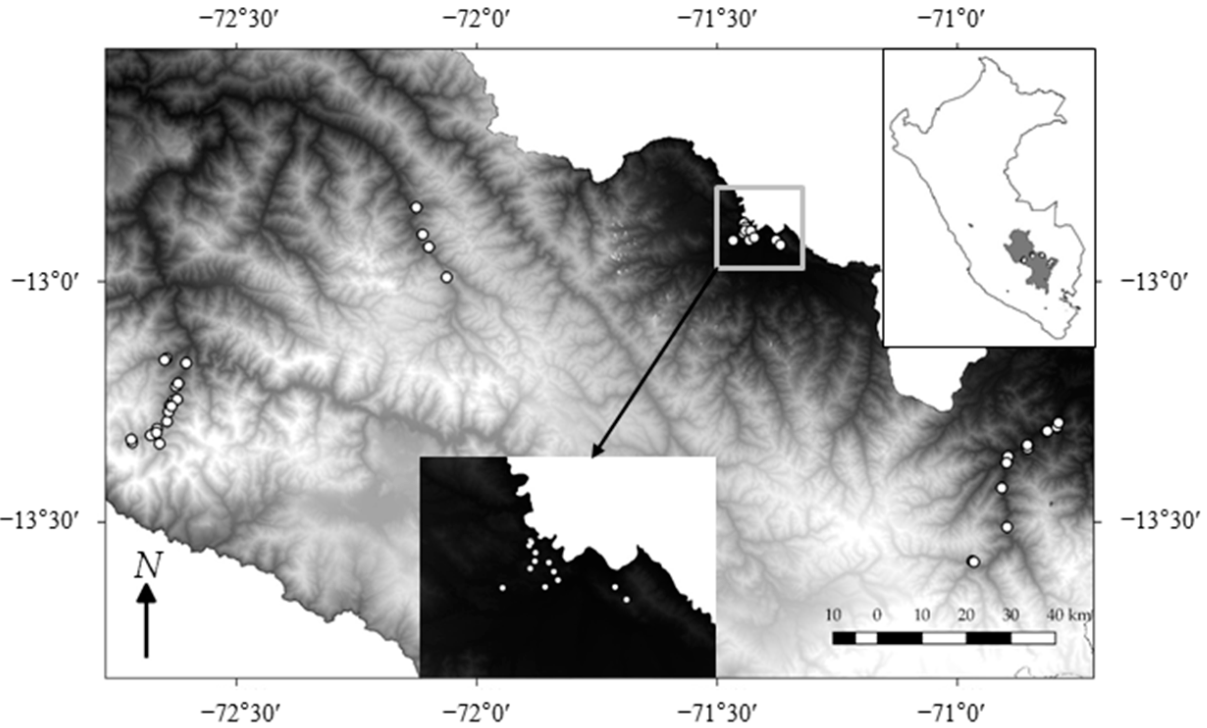
2.1. Study Sites

Study sites were located in Cusco region, Peru, with the area ranging from 12°50′ S to 13°34′ S and from 70°47′ W to 72°40′ W (Figure 1). Our study was mainly conducted in upland tropical forest and partly in montane forest. Climate conditions are variable along the elevational gradient that ranges from ca. 600 m a.s.l. in upland tropical forest to ca. 3500 m a.s.l. in montane forest. Mean annual air temperature and mean annual rainfall are 23.1 °C and 5016 mm at Quince Mil at 644 m a.s.l., and 12.8 °C and 765 mm at Marcapata at 3110 m a.s.l. [22].

2.2. Field Survey

We established 45 plots in Cusco region from August 2015 to February 2017. The elevation of the plots ranged from 584 to 3535 m. The plot size was 40 m × 40 m, with the exception of two of 40 m × 20 m and one of 30 m × 15 m. The field survey data of these smaller plots were included only in the biomass and carbon stock estimations. They were not used for the analyses of community composition to avoid the effect of difference in plot size on the number of species. Plot locations were selected to include a wide range of elevations, topographies, and natural and human disturbances (see the Supplementary Material, Table S1). The plots were separated by at least 500 m, and they were established at least 50 m from major roads.

Plot establishment and tree measurement followed the methods in a research manual used for ground-based forest inventory, the REDD-plus Cookbook Annex [23]. We measured diameter at breast height (1.3 m; DBH) of all trees ≥10 cm in DBH. We measured tree height (from the base to the top of the canopy) in two 10 m × 10 m subplots for trees 5 to 10 cm in DBH and in four subplots for trees ≥10 cm in DBH. Trees were identified to at least the family level (and ideally to the species level) in the field. When there were difficulties, voucher specimens and photographs were collected for identification by specialists in the laboratory of the Servicio Nacional Forestal y de Fauna Silvestre, in Lima.

We qualitatively classified the surveyed forest stands into primary and secondary forests. We defined primary forest as a forest that includes late-successional tree species in the forest canopy with no evidence of clear cut in the past (i.e., no evidence of second growth). In the field, we checked presence of late-successional species (e.g., Pouteria lucuma (Ruiz & Pav.) Kuntze, Sapotaceae) based on our experience and literature [24]. Our primary forest stands had no evidence of clear cut, but most of them were partly subject to human disturbances such as selective logging. Although a field manual of National Forest Inventory in Peru [25] distinguishes this forest type as ‘disturbed primary forest’ from intact primary forest with no influence of human activities, here we call it just ‘primary forest’ to avoid terminological confusion. We defined secondary forest as a forest primarily characterized by evidence of clear felling and second growth, and partly by presence of pioneer species (e.g., Heliocarpus americanus L., Marvaceae; Trema micrantha (L.) Blume, Cannabaceae).

We also measured coarse woody debris (CWD), which we defined as all dead woody fragments ≥10 cm in diameter, to increase the accuracy of carbon stock estimation in each plot. We classified CWD into three categories: Stump, fallen dead tree, and standing dead tree. We measured the diameter and length (or height of standing trees) of all CWD ≥ 10 cm in diameter to estimate their volume. We assumed that the stem sections were cylinders with averaged cross-sectional area. We measured the diameters of the cut surface of stumps, diameters at both ends of fallen trees, and DBH in standing dead trees to obtain the averaged cross-sectional area. According to the definition of Chao et al. [26], one of the three decomposition classes (class 1–3) was recorded for each CWD piece based on field observation (see Equation (3) for dead wood mass, below).

Environmental conditions such as elevation and topographies and evidence of natural and human disturbances observed in and around the forest plots were recorded. The natural disturbances included erosion and wind, whereas the human disturbances included logging, fire and crop cultivation. We recorded evidence of these disturbances during and just after field survey for each plot, on the basis of the direct observations and interviews with local residents (see the Supplementary Material, Table S1).

2.3. Estimation of Biomass, CWD, and Total Carbon Stock

We estimated AGB (kg) at an individual-tree level using the following generic equation [27]:

AGB = 0.0673 × (WD × D²H)^0.976

(1)

where WD is the wood density (g cm⁻³), D is the DBH (cm), and H is the tree height (m). For trees that lacked a height measurement, we estimated H using a DBH–tree height allometric relationship based on the sampled measurements in each plot. We used Global wood density database [28] to assign a wood density value to each tree by the species, genus or family identification. For unidentified trees, we used the default value (0.60 g cm⁻³) for tropical America [29]. We summed the AGB of all live trees in each plot, then converted into the stand-level AGB (AGB_h, Mg ha⁻¹).

We estimated below-ground biomass (BGB) at a plot level as [30]:

BGB_h = 0.489 × AGB_h^0.890

(2)

where BGB_h and AGB_h are the stand-level BGB and AGB estimates per hectare (Mg ha⁻¹).

The dead wood mass of CWD (g) was estimated at a plot level as:

Dead wood mass of CWD = V × WD_d

(3)

where V is the volume of CWD measured in the field (cm³), and WD_d is the wood density of CWD (g cm⁻³). WD_d was determined by using three decomposition classes for CWD (0.55, 0.41 and 0.23 g cm⁻³, for decomposition class 1–3, respectively) [26].

Total carbon stock (MgC ha⁻¹) was obtained at a plot level as:

Total carbon stock = (AGB_h + BGB_h + total CWD) × CF

(4)

where CF denotes the carbon fraction of dry matter, 0.47 [31].

2.4. Analyses of Community Composition and Species Richness

We performed non-metric multidimensional scaling (NMDS) to examine differences in community composition among the plots. In this analysis, community composition was represented by the scores along the two NMDS axes. Genus-level abundance data (i.e., stem density) were used to represent the community-level data in this analysis because tree identification was limited to genus in many cases. Previous studies [10] using the NMDS axes demonstrated that the community composition data at genus level was strongly correlated with those at species level, and suggested that genus-level identification was applicable to the evaluation of forest degradation. In addition, the community data were limited to the forty-two 40 m × 40 m plots to simplify interpretation of the results, excluding three smaller plots. The NMDS was performed using metaMDS function in ‘vegan’ package for R software and Chao index of similarity [32] based on community abundance data. The Chao index is one of the best options among similarity indices because it can consider the probability of rare species (genus in this study) in communities [33]. Associations between NMDS axis scores and environmental factors were evaluated with envfit function in the ‘vegan’ package. The environmental factors include elevation, topography, disturbances, forest type (primary forest vs. secondary forest) and forest characteristics. The disturbance factors included erosion and wind for natural disturbances, and logging, cultivation, fire and infrastructure such as trails and other artificial materials for human disturbances (see the Supplementary Material, Table S1). The forest characteristics include AGB, BGB, total CWD, total carbon, mean DBH, community-weighted mean (CWM) DBH and maximum DBH and mean tree height, CWM tree height and maximum tree height, species richness, CWM wood density, and Gini coefficients based on DBH and tree height (see the Supplementary Material, Table S2). The CWM DBH and CWM tree height are weighted means based on abundance data at genus level. The CWM wood density was also calculated in the same manner using the above-mentioned Global wood density database [28]. The Gini coefficient was used as an index of inequality of tree size (DBH or tree height) at stand level, and it can be obtained as:

$$\mathrm{Gini}\mathrm{coefficient}={\displaystyle {\sum }_{i=1}^n{\displaystyle {\sum }_{j=1}^n\left|x_i-x_j\right|/2n^2\mu }}$$

(5)

where x_i and x_j are individual trees i and j; n represents total number of trees and μ denotes mean tree size [34]. The Gini coefficient ranges from zero (all trees are completely equal in size) to one (dominated by a single tree), and it has an advantage for comparison between stands because it does not depend on tree density and total basal area (BA) [35].

Since our study plots have a long elevation range, change in AGB and community composition may merely reflect the changes across different vegetation zones. To minimize the elevation effects on AGB and community composition, we classified our plots into different elevation zones using tree models in package ‘tree’ for R software (v. 3.4.4, R Foundation for Statistical Computing, Vienna, Austria), based on NMDS axis 1 scores for the response variable. The explanatory variables were the same as environmental factors for the NMDS as described above. This classification causes smaller sample size for each elevation zone, and may be difficult to obtain clear results with statistical significance. Therefore, the following analyses were performed using all data combined and classified data.

To explore abiotic and biotic factors that could affect the variation in community composition for the whole elevation range and each of the classified elevation zones, we performed generalized linear models (GLMs) for multivariate abundance data, using manyglm function in package ‘mvabund’ for R software [36]. This approach can cope with the issue of misspecification of the mean—variance relationships in community data that was not handled by the distance-based (or dissimilarity-based) analyses. It is a flexible and powerful approach for analyzing community data [36,37]. We specified negative-binomial family for all cases by checking the residuals vs. fits pattern. The environmental factors and forest characteristics tested are as mentioned above (see Supplementary Materials, Tables S1 and S2). To test the effect of these variables other than elevation, we compared the model fits between null and alternative models. We set the null model as a model that included elevation alone, and the alternative model as a model that added one of the variables as well as elevation. Model comparison was performed by analysis of deviance and Akaike Information Criterion (AIC) using anova.manyglm function in package ‘mvabund’. The p-values for the effect of each variable in the alternative model were obtained by 1000 times Bootstrap resampling of a log-likelihood ratio under the null model.

We calculated the species richness per plot as the average number of species per 10 trees sampled from each plot data using 1000 randomizations, because the number of species per plot can increase with increasing tree density [10,38]. Tree species (or genera) were categorized into pioneer species and late-successional species. In practice, however, this categorization is not simple because information about the successional status of each species is incomplete. Because wood density is known as a key trait associated with a species’ successional status [24,39], we defined tree species with WD < 0.40 g cm⁻³ as pioneer species and those with WD ≥ 0.64 g cm⁻³ as late-successional species on the basis of previously published data [24,39].

Data manipulation and statistical analyses were conducted in R software (v. 3.4.4) [40] and the ‘mvabund’, ‘tree’ and ‘vegan’ packages for community ecology analyses.

3. Results

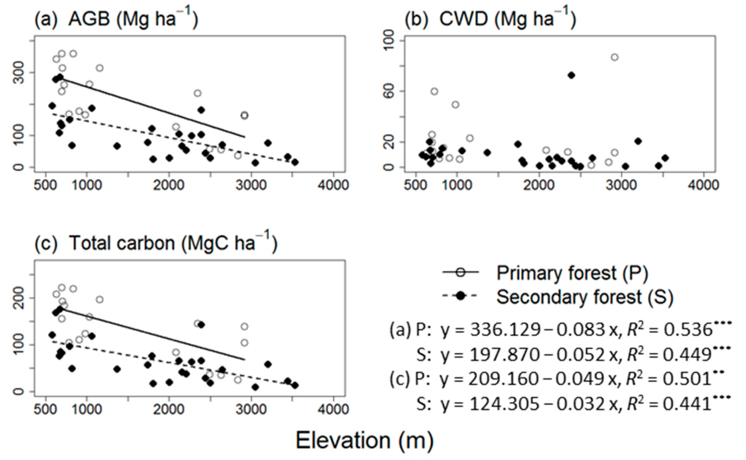
3.1. AGB, CWD, and Total Carbon Stock

AGB decreased with increasing elevation in both primary and secondary forests (Figure 2a). It was significantly greater in primary forest than in secondary forest (ANCOVA, p < 0.001 for comparison of the regression intercepts). However, the range overlapped between the two forest types (from 35.1 to 358.3 Mg ha⁻¹ in primary forest and from 12.9 to 284.5 Mg ha⁻¹ in secondary forest). CWD was not significantly related to elevation (ANCOVA, p ≥ 0.05; Figure 2b), and it was not significantly different between forest types (the mean values of 20.9 Mg ha⁻¹ in primary forest and 10.0 Mg ha⁻¹ in secondary forest; t-test p ≥ 0.05). As a consequence, the total carbon stock (including AGB, BGB and CWD) followed the same declining trend with elevation as AGB, with a greater mean value in primary forest (135.2 MgC ha⁻¹) than in secondary forest (66.3 MgC ha⁻¹; ANCOVA, p < 0.001; Figure 2c). It ranged from 24.2 to 221.1 MgC ha⁻¹ in primary forest and from 8.6 to 175.4 MgC ha⁻¹ in secondary forest. AGB, BGB, and CWD accounted for ca. 71.4%, 21.6%, and 7.0% of the total carbon stock, on average.

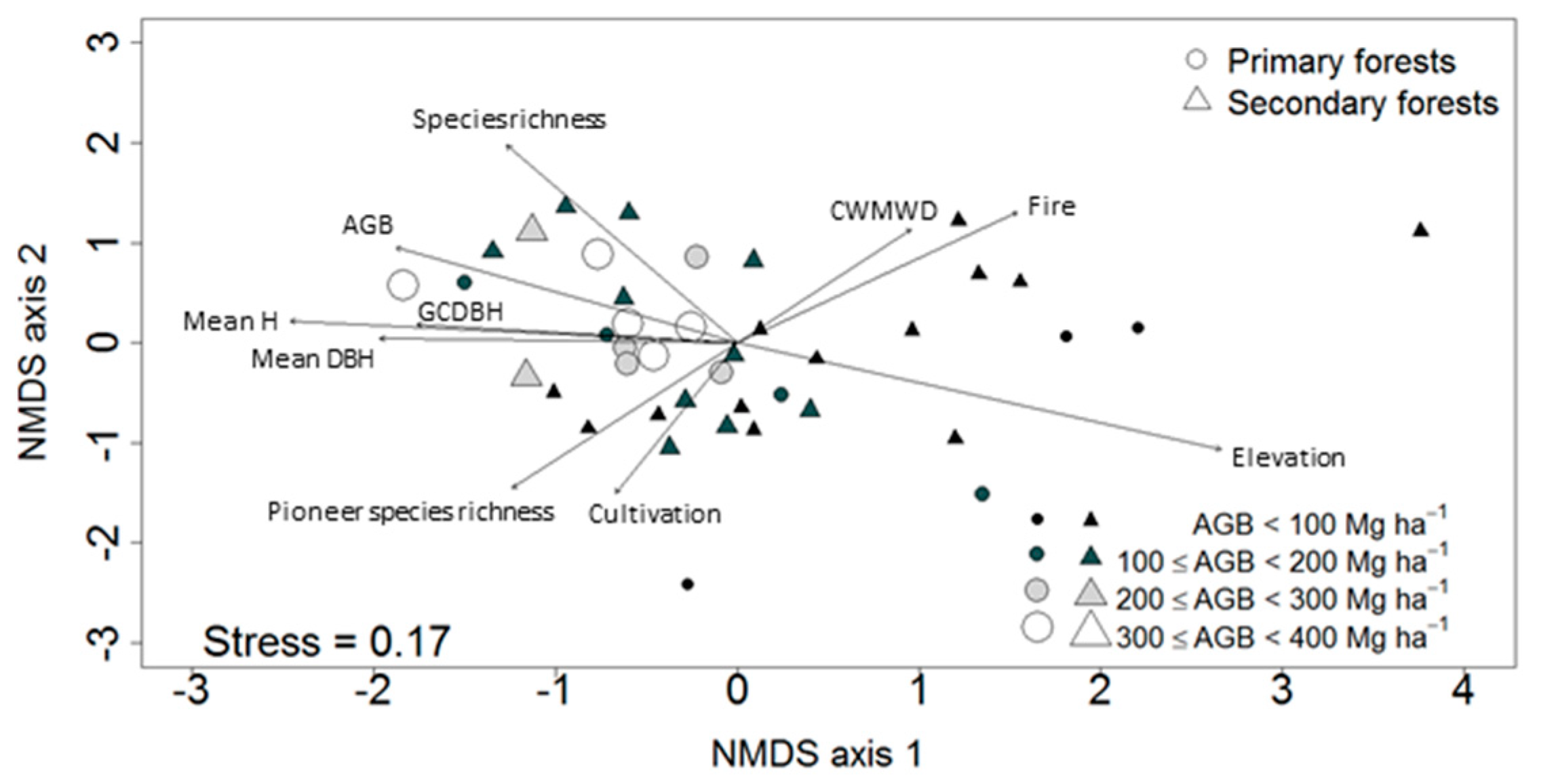
3.2. Ordination of the Study Plots

The NMDS based on community abundance data demonstrated that the plots with greater AGB at lower elevation and those with lower AGB at higher elevation were positioned mainly along the NMDS axis 1 (Figure 3). The BGB and total carbon showed associations which were very similar to that of AGB (only AGB was shown in Figure 3 because arrows were overlapped). Mean DBH, mean tree height and Gini coefficient (DBH basis) had similar directions to that of AGB, and showed significant associations with NMDS axis scores. Other tree size metrics including max. DBH, CWM DBH, max. tree height, CWM tree height, Gini coefficient (tree height basis) also showed significant but slightly weak associations. Species richness (all species and pioneers), CWM wood density and disturbances (cultivation and fire) showed significant associations with NMDS axis scores, but their directions were different from that of AGB. Forest type (primary forest vs. secondary forest) and other environmental and forest characteristics (topography, erosion, wind, logging, infrastructure, total CWD) were not significantly associated with the NMDS axis scores.

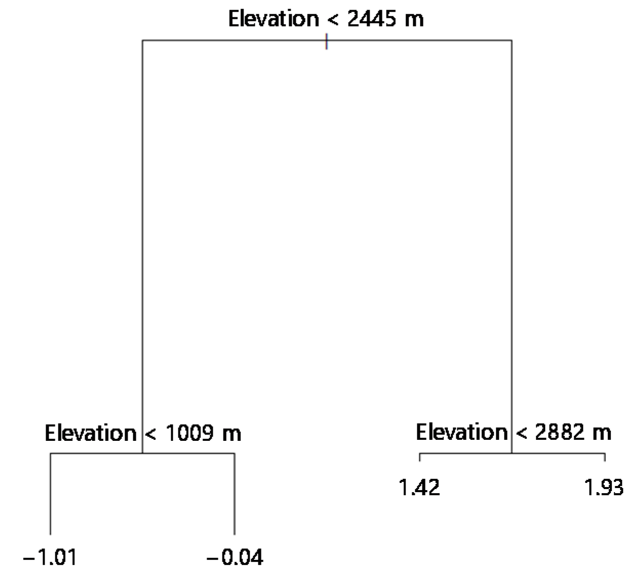
3.3. Classification of Different Elevation Zones

As shown in Figure 3, change in community composition was strongly affected by elevation. To minimize the elevation effect and to detect the factors affecting the variations in community composition other than elevation, we performed the tree model analysis based on NMDS axis 1 scores. The results showed that our study plots were primarily classified by elevation rather than other environmental factors including topography and natural and human disturbances (Figure 4). The important elevation thresholds were 2445 m followed by 1009 m and 2882 m. According to this result, we divided the study plots into three elevation zones using the first two thresholds: low elevation (<1000 m), mid elevation (1000–2400 m) and high elevation (≥2400 m). We did not use 2882 m as a threshold because of its lesser importance (suggested by the shorter vertical lines in the tree model, Figure 4) and insufficient number of plots.

3.4. Factors Affecting Community Composition

The results of model comparisons for testing the effects of environmental factors on community composition are shown in

Table 1. Summary of model comparisons between elevation effect alone and elevation effect plus one of the other environmental effects across the whole elevation range of sampled forest sites in the Cusco region of Peru.

Variables	Whole Elevation Range (584–3535 m) n = 41 (df 39 vs. 38, 32) a
	LR b	AIC c	ΔAIC d
Elevation (m)	—	6174	—
+ Cultivation	266.0 *	6266	92
+ Erosion	248.7 *	6284	109
+ Fire	125.8	6407	232
+ Infrastructure	250.1 *	6282	108
+ Logging	234.1	6298	124
+ Wind	159.9	6373	198
+ Topography	907.6 *	7773	1598

Significance level: * p < 0.05; ^a df of two models (df 39 for elevation effect alone and df 38 for elevation effect plus one of the other environmental effects, except df 32 for the model including topography) are shown in the parentheses; ^b LR: Log likelihood ratio; ^c AIC: Akaike Information Criterion; ^d ΔAIC: difference from AIC of the model with elevation effect alone; Inconsistency between ΔAIC and the one based on difference in AIC of two models is due to rounding. Dash indicates data is not applicable.

and

Table 2. Summary of model comparisons between elevation effect alone and elevation effect plus one of the other environmental effects at three elevation sites.

Variables	Low Elevation (<1000 m) n = 16 (df 14 vs. 13, 9) a			Mid Elevation (1000–2400 m) n = 15 (df 13 vs. 12, 10) a			High Elevation (≥2400m) n = 10 (df 8 vs. 7, 5) a
	LR	AIC	ΔAIC	LR	AIC	ΔAIC	LR	AIC	ΔAIC
Elevation (m)	—	2730	—	—	2085	—	—	1009	—
+ Cultivation	115.7	2840	110	87.4	2148	63	48.4	1059	50
+ Erosion	233.0 **	2723	−7	115.5 †	2120	34	21.8	1085	76
+ Fire	NA	NA	NA	NA	NA	NA	81.1	1026	17
+ Infrastructure	133.0 †	2823	93	69.2	2166	81	133.6 *	973	−36
+ Logging	108.6	2847	117	96.5	2139	54	87.7	1019	10
+ Wind	83.8	2872	142	126.4 †	2109	24	NA	NA	NA
+ Topography	587.6 **	3497	768	250.9 *	2585	499	223.8 †	1275	266

Significance levels: ^† p < 0.1; * p < 0.05; ** p < 0.01; ^a df of two models (from low to high elevation: df 14, 13 and 8 for elevation effect alone and df 13, 12 and 7 for elevation effect plus one of the other environmental effects, except df 9, 10 and 5 for the model including topography) are shown in the parentheses; NA, not applicable due to no “presence” observation. Dash indicates data is not applicable.

. When considering the whole elevation range, cultivation, erosion, infrastructure and topography had a significant effect (p < 0.05) but these showed a higher AIC than the null model (i.e., elevation alone). No environmental factors lowered AIC of the alternative model compared with that of the null model (Table 1). On the other hand, in each of the classified elevation zones, erosion had a significant effect and lower AIC compared with the null model at low elevation, while infrastructure showed a significant effect and lowered AIC at high elevation (Table 2). Trace of fire was observed only in three plots at high elevation, and the effect was not significant. Other factors including cultivation, logging, wind and topography had no significant effect, nor did they lower AIC of the model.

Table 3. Summary of model comparisons between elevation effect alone and elevation effect plus one of forest characteristics effects for a whole elevation range.

Variables b	Whole Elevation Range (584–3535 m) n = 41 (df 39 vs. 38) a
	LR	AIC	ΔAIC
Elevation (m)	—	6174	—
+ Forest type (primary/secondary)	322.4 **	6210	36
+ BA (m ha−1)	257.5 *	6275	101
+ AGB (Mg ha−1)	274.5 †	6258	83
+ BGB (Mg ha−1)	273.1 †	6259	85
+ Total CWD (Mg ha−1)	224.6	6308	133
+ Total carbon (MgC ha−1)	279.9 *	6252	78
+ CWM wood density (g cm−3)	272.1 *	6260	86
+ Mean DBH (cm)	187.2	6345	170
+ CWM DBH (cm)	173.4	6359	185
+ Max. DBH (cm)	233.1 †	6299	125
+ Mean tree height (m)	341.1 **	6191	17
+ CWM tree height (m)	186.2	6346	172
+ Max. tree height (m)	329.8 **	6203	28
+ Species richness (all species) c	307.9 **	6219	44
+ Species richness (pioneers) c	356.5 **	6176	1
+ Species richness (late-successional) c	294.5 *	6238	64
+ Gini coefficient (DBH basis)	230.1	6302	128
+ Gini coefficient (Tree height basis)	180.9	6352	177

Significance levels: ^† p < 0.1; * p < 0.05; ** p < 0.01; ^a df of two models (elevation effect alone and elevation effect plus one of forest characteristics effects) are shown in the parentheses; ^b Abbreviations: BA, basal area; CWD, coarse woody debris; CWM, community-weighted mean based on abundance; ^c Species richness was calculated as the average number of species per 10 trees randomly sampled from each plot (see Section 2). Dash indicates data is not applicable.

and

Table 4. Summary of model comparisons between elevation effect alone and elevation effect plus one of forest characteristics effects at three elevation sites.

Variables b	Low Elevation (<1000 m) n = 16 (df 14 vs. 13) a			Mid Elevation (1000–2400 m) n = 15 (df 13 vs. 12) a			High Elevation (≥2400m) n = 10 (df 8 vs. 7) a
	LR	AIC	ΔAIC	LR	AIC	ΔAIC	LR	AIC	ΔAIC
Elevation (m)	—	2730	—	—	2085	—	—	1009	—
+ Forest type (primary/secondary)	174.9 †	2781	51	125.4 †	2110	25	73.3	1034	25
+ BA (m ha−1)	167.0 †	2789	59	183.8 *	2052	−34	90.0	1017	8
+ AGB (Mg ha−1)	160.2	2796	66	206.1 *	2029	−56	41.3	1066	57
+ BGB (Mg ha−1)	160.3	2795	66	203.2 *	2032	−53	41.5	1065	56
+ Total CWD (Mg ha−1)	125.3	2830	101	194.9 *	2040	−45	50.2	1057	48
+ Total carbon (MgC ha−1)	162.4	2793	64	200.7 *	2035	−51	41.9	1065	56
+ CWM wood density (g cm−3)	140.9	2815	85	185.7 *	2050	−36	108.4	998	−10
+ Mean DBH (cm)	131.5	2824	94	256.5 **	1979	−107	52.9	1054	45
+ CWM DBH (cm)	129.2	2827	97	212.6 **	2023	−63	53.4	1053	45
+ Max. DBH (cm)	149.8 †	2806	76	205.7 **	2030	−56	33.6	1073	64
+ Mean tree height (m)	243.6 **	2713	−17	251.7 **	1984	−102	111.6	995	−14
+ CWM tree height (m)	133.6	2822	92	155.5 †	2080	−6	105.0	1002	−7
+ Max. tree height (m)	166.9 †	2789	59	282.9 ***	1952	−133	101.4 *	1005	−3
+ Species richness (all species) c	184.7 *	2771	41	190.5 *	2045	−41	188.4 **	919	−90
+ Species richness (pioneers) c	247.0 **	2709	−21	140.6	2095	9	155.1 *	952	−57
+ Species richness (late-successional) c	240.9 **	2715	−15	108.4	2127	42	108.7	998	−11
+ Gini coefficient (DBH basis)	135.4	2820	91	207.8 **	2028	−58	83.5	1023	15
+ Gini coefficient (Tree height basis)	141.6	2814	81	180.7 †	2055	−31	86.4	1020	12

Significance levels: ^† p < 0.1; * p < 0.05; ** p < 0.01; *** p < 0.001; ^a df of two models (elevation effect alone and elevation effect plus one of forest characteristics effects) are shown in the parentheses; ^b Abbreviations: BA, basal area; CWD, coarse woody debris; CWM, community-weighted mean based on abundance; ^c Species richness was calculated as the average number of species per 10 trees randomly sampled from each plot (see Section 2). Dash indicates data is not applicable.

show the results of model comparisons for testing the effects of forest characteristics on community composition. In the whole elevation range, forest type, BA, total carbon, mean and maximum tree height and species richness including pioneer and late-successional species showed a significant effect (p < 0.05), but no forest characteristics lowered AIC of the model compared with the null model (Table 3). In the case of the classified elevation zones, mean tree height had a significant effect at low and mid elevations, and showed a consistently lower AIC than the null model across all elevations (Table 4). Maximum tree height and species richness (all species) lowered AIC with a significant factor effect at mid and high elevations. Species richness of both pioneers and late-successional species showed a lower AIC with a significant effect at low and high elevations, except the effect of species richness of late-successional species was not significant at high elevation. A significant effect (p < 0.05 to p < 0.001) with a lower AIC was observed for many factors only at mid elevation: carbon stock-related measures (BA, AGB, BGB, total CWD and total carbon), CWM wood density, DBH (mean, CWM and maximum), tree height (mean and maximum), species richness (all species) and Gini coefficient (DBH basis).

With respect to changes in species richness along an elevation gradient, species richness of pioneers and late-successional species showed no significant correlation with elevation, although a significant negative correlation was found between species richness of pioneers and elevation only when the data was limited to >1000 m a.s.l. (Spearman’s rank correlation coefficient r_s = −0.53, p < 0.01; see the Supplementary Material, Figure S1).

4. Discussion

This study demonstrated the variation in AGB and carbon stocks across the wide elevation gradient in the Andean region. Our results also suggest that the community composition in our study plots was affected by natural and human disturbances and forest characteristics. When considering the whole elevation range, however, neither environmental factors nor forest characteristics showed a lower AIC in the model including each of themselves compared with the model including the effect of elevation alone (Table 1 and Table 3). This result indicates that the associations between community composition and environmental factors and forest characteristics detected in the NMDS analysis (Figure 3) may reflect a shift from one vegetation zone to another along an elevation gradient. When focusing on each of the classified elevations, different factors affected community composition at the different elevations: natural disturbance (erosion) appeared to be a major factor at low elevation, whereas human disturbance (infrastructure) was likely to affect community composition at high elevation (Table 2). With respect to forest characteristics that affect community composition (Table 4), tree height measures, particularly mean tree height, showed a relatively consistent effect on community composition across the different elevations.

The range of total carbon stocks (including AGB, BGB and CWD) (24.2 to 221.1 MgC ha⁻¹ for primary forest and 8.6 to 175.4 MgC ha⁻¹ for secondary forest) was wider than those of previous studies in Andean forests [21,41], reflecting the wider elevation range in our study plots. For example, a transect study ranging from 1050 to 3060 m a.s.l. in an Ecuadorian forest demonstrated that carbon stock (above- and belowground, but not including CWD) decreased from 153.6 to 66.5 MgC ha⁻¹ with increasing elevation [41]. In addition, the difference between our study and these previous studies may be because our plots include disturbed forests with various degrees of human disturbance. The mean CWD mass and carbon stock (20.9 Mg ha⁻¹ and 9.8 MgC ha⁻¹ in primary forest and 10.0 Mg ha⁻¹ and 4.7 MgC ha⁻¹ in secondary forest) in this study were within the range of CWD carbon stock of Andean forests in previous studies although they contain high variations (0.2–12 MgC ha⁻¹ in Ecuador [42]; 1.8 and 23.1–56.4 MgC ha⁻¹ in Peru [21,43]). On average, the CWD of our plots contributed 7.0% to the total carbon stock. In general, CWD stocks account for up to 33% of biomass of trees ≥10 cm in tropical forests [44]. One possible explanation of the lower contribution of CWD stocks in this study is that fallen trees and twigs may be taken away more often from the forests and utilized for fuelwood.

In this study, we did not detect clear differences in AGB and community composition between primary and secondary forests (Figure 2 and Figure 3, Table 1). The reason for the results was partly because our primary forest plots were subject to different degrees of human disturbances. As a result, AGB and community composition may become similar between the two forest types. As an example of quantifying human disturbances, Toivonen et al. [15] reported that in Andean highland forests above 3300 m a.s.l., forest characteristics including mean and maximum tree height decreased with increasing human disturbance, represented by ‘accessibility’, distance to the nearest road, village and market. Thus, different degrees of human disturbance can promote variation in forest structure, and eventually influence AGB and community composition.

In terms of the environmental factors, erosion (a natural disturbance) had a significant effect on community composition and showed a lower AIC in the model at low elevation, whereas infrastructure (a human disturbance) was detected as a major factor at high elevation (Table 2). Clark et al. [45] found that the landslide rate was increasing with decreasing elevation from 4000 to 1000 m a.s.l. in Andean forests which may be associated with higher rainfall at lower elevation. Although elevation range was slightly different from this study, the trend generally agrees with our result (Table 2). A similar mechanism related to rainfall may also influence the incidence of erosion at low elevation in our plots.

Infrastructure such as sheds and trails nearby forests is considered to represent relatively high human activity and accessibility. In our plots, presence of infrastructure partly coincided with evidences of crop cultivation, fire and logging. Previous studies pointed out that unofficial fine roads that were first built for logging, can be a major driver of deforestation and forest degradation, providing entry points for human colonization and other land use such as agriculture lands [46,47]. The high Andes region in Peru has been under the influence of human population with land use change both through agriculture and fire [21]. Crop cultivation such as of beans, corns, and potatoes is popular in the agricultural landscapes. A recent study reported that rapid land use change including deforestation had a great impact on soil fertility and biodiversity, and threatened the sustainability of farming in this region [48]. Although crop cultivation and fire were significantly associated with community composition only in the NMDS analysis (Figure 3) and not in GLMs for multivariate abundance data (Table 1, Table 2, Table 3 and Table 4), it has been reported that Andean montane forests are suffering from human-induced fires which start in the flammable grassland region (locally called Puna) at relatively high elevation (>2000 m a.s.l.) [21]. In this study, however, we observed evidence of fire only in three plots. More data are required to evaluate the effect of fires on the Andean montane forests. Although our finding is currently limited, this study suggests that natural and human disturbances would affect the variation in community composition in Andean forests across the different elevations.

In terms of forest characteristics that are associated with community composition, mean tree height showed a relatively consistent correlation across different elevations (Table 4). This suggests that change in community composition would at least partly bring about change in forest (canopy) structure. A previous study in Borneo demonstrated that tree height was a useful indicator to evaluate forest degradation, as tree height was correlated with the similarity in community composition that reflected different degrees of human disturbances [11]. Our results especially at high elevation are in accordance with the previous finding.

Many forest characteristics had a significant effect on community composition and lowered AIC in the model at mid elevation (Table 4). The reason for the result is because this elevation zone covers a wider range (1000–2400 m) compared with low (584–1000 m) and high (2400–3535 m) elevations in this study, and it probably contains a transition zone between the different vegetation zones. Therefore, within this elevation zone, there would be high variations in biomass (Figure 2), tree size, and species richness (Figure S1) that can be recognized to be associated with community composition.

Our analyses suggested that species richness at least partly accounted for variation in community composition across the plots, although its contribution seemed more prominent in all species or pioneers than in late-successional species (Figure 3, Table 4 and also see supplementary materials, Table S3). It might be important to note that our categorization of trees into pioneer and late-successional species was based only on wood density, since we lacked sufficient knowledge of the successional status of many species. A previous study that mapped carbon stock and identified the drivers of its regional variation in the Amazon basin demonstrated that Andean forests in Peru generally consisted of trees with low wood density [49]. This might indicate an inconsistency between our classification of successional status based on wood density and the actual successional status at our study sites. Although wood density is a key trait associated with species’ successional status [24,39], other key traits and more information about the ecological characteristics of each species might be required to reflect the actual successional status of the tree species in Andean forests. Imai et al. [10] pointed out that community composition is sensitive and more robust metric for evaluating forest degradation compared to species richness, because the relationship between species richness and a surrogate of forest degradation (AGB in their case) was non-linear and species richness peaked in moderately degraded forests. Thus, community composition might be a better indicator for evaluating forest degradation also in Andean forests.

In context of REDD+, the present results suggest that particular attention should be paid to REDD+ activities in high Andes region to mitigate anthropogenic greenhouse gas emissions, as the impact of human disturbances on community composition in the forests appeared to be more prominent at higher elevations. In addition, the assessment of forest degradation using community composition should be separately conducted for each of different vegetation zones, to avoid a misleading interpretation by the confounding effect of elevation reflecting the shift to a different vegetation zone.

5. Conclusions

The REDD+ safeguards are intended to emphasize the importance of forest biodiversity conservation and to protect biodiversity against ‘side effects’ derived from REDD+ activities within a climate change mitigation framework (e.g., converting natural forests into plantation forests of single fast-growing species to increase carbon fixation) [50]. In addition to this aspect of the safeguards, the present study suggested that under the influence of natural and human disturbances, the changes in community composition might be linked to the degradation of forest structure (i.e., mean tree height in the present study). Also, management efforts including biodiversity monitoring are an urgent need for biodiversity conservation in the high Peruvian Andes, an area susceptible to human disturbances and climate change [51]. Thus, forest biodiversity conservation will play an important role in the REDD+ activities in Andean forests. Meanwhile, previous studies suggested that tree height data based on field survey can contribute to more accurately predict large-area trends in AGB and total carbon stocks [50,52,53,54]. In this sense, mean tree height may have a potential to be a key measure for evaluating variations in both community composition and carbon stocks in Andean forests. Seeking and developing suitable indicators for representing biodiversity loss and changes in forest structure and carbon stocks will help evaluate forest degradation more accurately in the Peruvian Andes.

References

1. Smith, P.; Bustamante, M.; Ahammad, H.; Clark, H.; Dong, H.; Elsiddig, E.A.; Haberl, H.; Harper, R.; House, J.; Jafari, M.; et al. Agriculture, Forestry and Other Land Use (AFOLU). In Climate Change 2014: Mitigation of Climate Change. Contribution of Working Group III to the Fifth Assessment Report of the Intergovernmental Panel on Climate Change; Edenhofer, O., Pichs-Madruga, R., Sokona, Y., Farahani, E., Kadner, S., Seyboth, K., Adler, A., Baum, I., Brunner, S., Eickemeier, P., et al., Eds.; Cambridge University Press: Cambridge, UK; New York, NY, USA, 2014; pp. 811–922. [Google Scholar]
2. Strassburg, B.B.N.; Rodrigues, A.S.L.; Gusti, M.; Balmford, A.; Fritz, S.; Obersteiner, M.; Kerry Turner, R.; Brooks, T.M. Impacts of incentives to reduce emissions from deforestation on global species extinctions. Nat. Clim. Chang. 2012, 2, 350. [Google Scholar] [CrossRef]
3. Barlow, J.; Lennox, G.D.; Ferreira, J.; Berenguer, E.; Lees, A.C.; Nally, R.M.; Thomson, J.R.; Ferraz, S.F.D.B.; Louzada, J.; Oliveira, V.H.F.; et al. Anthropogenic disturbance in tropical forests can double biodiversity loss from deforestation. Nature 2016, 535, 144. [Google Scholar] [CrossRef] [PubMed]
4. United Nations Framework Convention on Climate Change. Report of the Conference of the Parties on Its Thirteenth Session; United Nations: New York, NY, USA, March 2008. [Google Scholar]
5. United Nations Framework Convention on Climate Change. Report of the Conference of the Parties on Its Sixteenth Session; United Nations: New York, NY, USA, March 2011. [Google Scholar]
6. Hirata, Y.; Takao, G.; Sato, T.; Toriyama, J. REDD-Plus Cookbook; REDD Research and Development Center, Forestry and Forest Products Research Institute: Tsukuba, Japan, 2012. [Google Scholar]
7. Gardner, T.A.; Burgess, N.D.; Aguilar-Amuchastegui, N.; Barlow, J.; Berenguer, E.; Clements, T.; Danielsen, F.; Ferreira, J.; Foden, W.; Kapos, V.; et al. A framework for integrating biodiversity concerns into national REDD+ programmes. Biol. Conserv. 2012, 154, 61–71. [Google Scholar] [CrossRef]
8. Kitayama, K. Co-Benefits of Sustainable Forestry: Ecological Studies of a Certified Bornean Rain Forest; Springer: Tokyo, Japan, 2013. [Google Scholar]
9. Pereira, H.M.; Ferrier, S.; Walters, M.; Geller, G.N.; Jongman, R.H.; Scholes, R.J.; Bruford, M.W.; Brummitt, N.; Butchart, S.H.; Cardoso, A.C.; et al. Essential biodiversity variables. Science 2013, 339, 277–278. [Google Scholar] [CrossRef] [PubMed] [Green Version]
10. Imai, N.; Tanaka, A.; Samejima, H.; Sugau, J.B.; Pereira, J.T.; Titin, J.; Kurniawan, Y.; Kitayama, K. Tree community composition as an indicator in biodiversity monitoring of REDD+. For. Ecol. Manag. 2014, 313, 169–179. [Google Scholar] [CrossRef]
11. Ioki, K.; Tsuyuki, S.; Hirata, Y.; Phua, M.H.; Wong, W.V.C.; Ling, Z.Y.; Johari, S.A.; Korom, A.; James, D.; Saito, H.; et al. Evaluation of the similarity in tree community composition in a tropical rainforest using airborne lidar data. Remote Sens. Environ. 2016, 173, 304–313. [Google Scholar] [CrossRef]
12. Aoyagi, R.; Imai, N.; Fujiki, S.; Sugau, J.B.; Pereira, J.T.; Kitayama, K. The mixing ratio of tree functional groups as a new index for biodiversity monitoring in Bornean production forests. For. Ecol. Manag. 2017, 403, 27–43. [Google Scholar] [CrossRef]
13. Laurance, W.F.; Goosem, M.; Laurance, S.G.W. Impacts of roads and linear clearings on tropical forests. Trends Ecol. Evol. 2009, 24, 659–669. [Google Scholar] [CrossRef] [PubMed] [Green Version]
14. Armenteras, D.; Retana, J. Dynamics, patterns and causes of fires in northwestern Amazonia. PLoS ONE 2012, 7, e35288. [Google Scholar] [CrossRef] [PubMed]
15. Toivonen, J.M.; Kessler, M.; Ruokolainen, K.; Hertel, D. Accessibility predicts structural variation of Andean Polylepis forests. Biodivers. Conserv. 2011, 20, 1789–1802. [Google Scholar] [CrossRef]
16. Toivonen, J.M.; Gonzales-Inca, C.A.; Bader, M.Y.; Ruokolainen, K.; Kessler, M. Elevational shifts in the topographic position of Polylepis forest stands in the Andes of southern Peru. Forests 2018, 9, 7. [Google Scholar] [CrossRef]
17. Ministerio del Ambiente (MINAM); Ministerio de Agricultura y Riego (MINAGRI). Memoria Descriptiva del Mapa de Ecozonas: Proyecto Inventario Nacional Forestal y Manejo Forestal Sostenible del Perú ante el Cambio Climático; MINAM and MINAGRI: Lima, Peru, 2014. (In Spanish)
18. Pickettet, S.T.A.; White, P.S. The Ecology of Natural Disturbance and Patch Dynamics; Academic Press: San Diego, CA, USA, 1985. [Google Scholar]
19. Ito, S. Forest formation and disturbance regime. In Forest Ecology; Masaki, T., Aiba, S., Eds.; Kyoritsu Shuppan: Tokyo, Japan, 2011; pp. 38–54. (In Japanese) [Google Scholar]
20. Barlow, J.; Peres, C.A. Ecological responses of Amazonian forests to El Niño-induced surface fires. In Tropical Forests and Global Atmospheric Change; Malhi, Y., Phillips, O.L., Eds.; Oxford University Press: Oxford, UK, 2005. [Google Scholar]
21. Román-Cuesta, R.M.; Salinas, N.; Asbjornsen, H.; Oliveras, I.; Huaman, V.; Gutierrez, Y.; Puelles, L.; Kala, J.; Yabar, D.; Rojas, M.; et al. Implications of fires on carbon budgets in Andean cloud montane forest: The importance of peat soils and tree resprouting. For. Ecol. Manag. 2011, 261, 1987–1997. [Google Scholar] [CrossRef]
22. Climate-Data.org. Climate: Cusco. Available online: https://en.climate-data.org/region/1060/ (accessed on 4 January 2018).
23. Sato, T.; Miyamoto, K. REDD-Plus Cookbook Annex. Research Manual Vol. 1 Ground-Based Inventory; REDD Research and Development Center, Forestry and Forest Products Research Institute: Tsukuba, Japan, 2016. [Google Scholar]
24. Chazdon, R.L.; Chao, A.; Colwell, R.K.; Lin, S.Y.; Norden, N.; Letcher, S.G.; Clark, D.B.; Finegan, B.; Arroyo, J.P. A novel statistical method for classifying habitat generalists and specialists. Ecology 2011, 92, 1332–1343. [Google Scholar] [CrossRef] [PubMed]
25. Ministerio de Agricultura y Riego (MINAGRI); Ministerio del Ambiente (MINAM). Manual de Campo–Ecozonas Costa y Sierra–Inventario Nacional Forestal: Proyecto Inventario Nacional Forestal y Manejo Forestal Sostenible ante el Cambio Climático en el Perú; MINAGRI and MINAM: Lima, Peru, 2015. (In Spanish)
26. Chao, K.-J.; Phillips, O.L.; Baker, T.R. Wood density and stocks of coarse woody debris in a northwestern Amazonian landscape. Can. J. For. Res. 2008, 38, 795–805. [Google Scholar] [CrossRef]
27. Chave, J.; Réjou-Méchain, M.; Búrquez, A.; Chidumayo, E.; Colgan, M.S.; Delitti, W.B.; Duque, A.; Eid, T.; Fearnside, P.M.; Goodman, R.C.; et al. Improved allometric models to estimate the aboveground biomass of tropical trees. Glob. Chang. Biol. 2014, 20, 3177–3190. [Google Scholar] [CrossRef] [PubMed]
28. Zanne, A.E.; Lopez-Gonzalez, G.; Coomes, D.A.; Ilic, J.; Jansen, S.; Lewis, S.L.; Miller, R.B.; Swenson, N.G.; Wiemann, M.C.; Chave, J. Data from: Towards a Worldwide Wood Economics Spectrum. Dryad Data Repository. 2009. Available online: https://doi.org/10.5061/dryad.234 (accessed on 6 June 2017).
29. Reyes, G.; Brown, S.; Chapman, J.; Lugo, A.E. Wood Densities of Tropical Tree Species; United States Department of Agriculture, Forestry Service, Southern Forest Experimental Station: New Orleans, LA, USA, 1992. [Google Scholar]
30. Mokany, K.; Raison, R.J.; Prokushkin, A.S. Critical analysis of root: Shoot ratios in terrestrial biomes. Glob. Chang. Biol. 2006, 12, 84–96. [Google Scholar] [CrossRef]
31. Aalde, H.; Gonzalez, P.; Gytarsky, M.; Krug, T.; Kurz, WA.; Ogle, S.; Raison, J.; Schoene, D.; Ravindranath, N.H.; Elhassan, N.G.; et al. Chapter 4: Forest Land. In 2006 IPCC Guidelines for National Greenhouse Gas Inventories, Prepared by the National Greenhouse Gas Inventories Programme, Volume 4 Agriculture, Forestry and Other Land Use; Eggleston, H.S., Buendia, L., Miwa, K., Ngara, T., Tanabe, K., Eds.; Institute for Global Environmental Strategies (IGES): Hayama, Japan, 2006; pp. 4.1–4.83. [Google Scholar]
32. Chao, A.; Chazdon, R.L.; Colwell, R.K.; Shen, T.J. A new statistical approach for assessing similarity of species composition with incidence and abundance data. Ecol. Lett. 2005, 8, 148–159. [Google Scholar] [CrossRef]
33. Doi, H.; Okamura, H. Similarity indices, ordination, and community analysis tests using the software R. Jpn. J. Ecol. 2011, 61, 3–20. (In Japanese) [Google Scholar]
34. Damgaard, C.; Weiner, J. Describing inequality in plant size or fecundity. Ecology 2000, 81, 1139–1142. [Google Scholar] [CrossRef]
35. Hakkenberg, C.R.; Song, C.; Peet, R.K.; White, P.S. Forest structure as a predictor of tree species diversity in the North Carolina piedmont. J. Veg. Sci. 2016, 27, 1151–1163. [Google Scholar] [CrossRef]
36. Wang, Y.; Naumann, U.; Wright, S.T.; Warton, D.I. mvabund—An R package for model-based analysis of multivariate abundance data. Methods Ecol. Evol. 2012, 3, 471–474. [Google Scholar] [CrossRef]
37. Warton, D.I.; Wright, S.T.; Wang, Y. Distance-based multivariate analyses confound location and dispersion effects. Methods Ecol. Evol. 2012, 3, 89–101. [Google Scholar] [CrossRef]
38. Gotelli, N.J.; Colwell, R.K. Quantifying biodiversity: Procedures and pitfalls in the measurement and comparison of species richness. Ecol. Lett. 2001, 4, 379–391. [Google Scholar] [CrossRef]
39. Plourde, B.T.; Boukili, V.K.; Chazdon, R.L. Radial changes in wood specific gravity of tropical trees: Inter- and intraspecific variation during secondary succession. Funct. Ecol. 2015, 29, 111–120. [Google Scholar] [CrossRef]
40. R Core Team. R: A Language and Environment for Statistical Computing; R Foundation for Statistical Computing: Vienna, Austria, 2018; Available online: http://www.R-project.org/ (accessed on 2 April 2018).
41. Moser, G.; Leuschner, C.; Hertel, D.; Graefe, S.; Soethe, N.; Iost, S. Elevation effects on the carbon budget of tropical mountain forests (S Ecuador): The role of the belowground compartment. Glob. Chang. Biol. 2011, 17, 2211–2226. [Google Scholar] [CrossRef]
42. Wilcke, W.; Yasin, S.; Abramowski, U.; Valarezo, C.; Zech, W. Nutrient storage and turnover in organic layers under tropical montane rain forest in Ecuador. Eur. J. Soil Sci. 2002, 53, 15–27. [Google Scholar] [CrossRef]
43. Gibbon, A.; Silman, M.R.; Malhi, Y.; Fisher, J.B.; Meir, P.; Zimmermann, M.; Dargie, G.C.; Farfan, W.R.; Garcia, K.C. Ecosystem carbon storage across the grassland-forest transition in the high Andes of Manu national park, Peru. Ecosystems 2010, 13, 1097–1111. [Google Scholar] [CrossRef]
44. Baker, T.R.; Honorio Coronado, E.N.; Phillips, O.L.; Martin, J.; van der Heijden, G.M.F.; Garcia, M.; Silva Espejo, J. Low stocks of coarse woody debris in a southwest Amazonian forest. Oecologia 2007, 152, 495–504. [Google Scholar] [CrossRef] [PubMed]
45. Clark, K.E.; West, A.J.; Hilton, R.G.; Asner, G.P.; Quesada, C.A.; Silman, M.R.; Saatchi, S.S.; Farfan-Rios, W.; Martin, R.E.; Horwath, A.B.; et al. Storm-triggered landslides in the Peruvian Andes and implications for topography, carbon cycles, and biodiversity. Earth Surf. Dyn. 2016, 4, 47–70. [Google Scholar] [CrossRef] [Green Version]
46. Barber, C.P.; Cochrane, M.A.; Souza, C.M.; Laurance, W.F. Roads, deforestation, and the mitigating effect of protected areas in the Amazon. Biol. Conserv. 2014, 177, 203–209. [Google Scholar] [CrossRef]
47. Kleinschroth, F.; Healey, J.R. Impacts of logging roads on tropical forests. Biotropica 2017, 49, 620–635. [Google Scholar] [CrossRef]
48. De Valenca, A.W.; Vanek, S.J.; Meza, K.; Ccanto, R.; Olivera, E.; Scurrah, M.; Lantinga, E.A.; Fonte, S.J. Land use as a driver of soil fertility and biodiversity across an agricultural landscape in the central Peruvian Andes. Ecol. Appl. 2017, 27, 1138–1154. [Google Scholar] [CrossRef] [PubMed]
49. Mitchard, E.T.A.; Feldpausch, T.R.; Brienen, R.J.W.; Lopez-Gonzalez, G.; Monteagudo, A.; Baker, T.R.; Lewis, S.L.; Lloyd, J.; Quesada, C.A.; Gloor, M.; et al. Markedly divergent estimates of Amazon forest carbon density from ground plots and satellites. Glob. Ecol. Biogeogr. 2014, 23, 935–946. [Google Scholar] [CrossRef] [PubMed] [Green Version]
50. Goetz, S.J.; Hansen, M.; Houghton, R.A.; Walker, W.; Laporte, N.; Busch, J. Measurement and monitoring needs, capabilities and potential for addressing reduced emissions from deforestation and forest degradation under REDD+. Environ. Res. Lett. 2015, 10. [Google Scholar] [CrossRef]
51. Lutz, D.A.; Powell, R.L.; Silman, M.R. Four decades of Andean timberline migration and implications for biodiversity loss with climate change. PLoS ONE 2013, 8, 1–9. [Google Scholar] [CrossRef] [PubMed]
52. Girardin, C.A.J.; Malhi, Y.; Aragao, L.; Mamani, M.; Huasco, W.H.; Durand, L.; Feeley, K.J.; Rapp, J.; Silva-Espejo, J.E.; Silman, M.; et al. Net primary productivity allocation and cycling of carbon along a tropical forest elevational transect in the Peruvian Andes. Glob. Chang. Biol. 2010, 16, 3176–3192. [Google Scholar] [CrossRef] [Green Version]
53. Baccini, A.; Goetz, S.J.; Walker, W.S.; Laporte, N.T.; Sun, M.; Sulla-Menashe, D.; Hackler, J.; Beck, P.S.A.; Dubayah, R.; Friedl, M.A.; et al. Estimated carbon dioxide emissions from tropical deforestation improved by carbon-density maps. Nat. Clim. Chang. 2012, 2, 182–185. [Google Scholar] [CrossRef]
54. Ioki, K.; Tsuyuki, S.; Hirata, Y.; Phua, M.-H.; Wong, W.V.C.; Ling, Z.-Y.; Saito, H.; Takao, G. Estimating above-ground biomass of tropical rainforest of different degradation levels in northern Borneo using airborne lidar. For. Ecol. Manag. 2014, 328, 335–341. [Google Scholar] [CrossRef]
Figure 1. Location of the study plots (open circles). The color gradient from black to white indicates low to high elevation. The insets show the location of Cusco region (gray) in Peru (top right) and the enlarged view of plot locations in Pillcopata region (bottom).
Forests 09 00390 g001
Figure 2. Relationships of elevation with (a) aboveground biomass (AGB), (b) coarse woody debris (CWD), and (c) the total carbon stock for the sampled forest sites in the Cusco region of Peru. Solid and dashed lines denote significant linear regressions. Significance levels: ** p < 0.01; *** p < 0.001.
Forests 09 00390 g002
Figure 3. NMDS (non-metric multidimensional scaling) ordination for the study plots. Arrows indicate the environmental and forest characteristics which are significantly associated with NMDS axis scores (envfit function, p < 0.05). Abbreviations: CWMWD, community-weighted mean wood density; GCDBH, Gini coefficient (DBH basis); MeanH, mean tree height.
Forests 09 00390 g003
Figure 4. Classification of the study plots by elevation using tree model. The values indicate mean NMDS 1 axis score for each group.
Forests 09 00390 g004