Models for Predicting Specific Gravity and Ring Width for Loblolly Pine from Intensively Managed Plantations, and Implications for Wood Utilization

Abstract

Loblolly pine (Pinus taeda L.) is increasingly grown on intensively managed plantations that yield high growth rates. Wood properties, including specific gravity (SG), change with cambial age, and thus intensively managed trees contain a high proportion of low density corewood when harvested because of reduced rotation lengths. This study was undertaken to develop models of ring-level properties (SG and width) in intensively managed loblolly pine plantations. Ninety-three trees from five stands aged from 24 to 33 years were harvested, and 490 disks were obtained from in between the 5.2-m logs that were cut, and at the merchantable top. The disks were cut into pith-to-bark radial strips that were scanned on an X-ray densitometer, and the resultant data analyzed using non-linear mixed-effects models. The fixed effects of the models, which included cambial age and for some models disk height and ring width, were able to explain 56, 46, 54, 16, and 46 percent of the within-tree variation for ring SG, ring width, latewood SG, earlywood SG, and latewood percent, respectively. To assess implications for wood utilization, a modeled tree was built by using height, diameter, and taper equations and these models were linked with the developed ring SG model to produce a tree properties map. The linked information was also used to generate tree and log SG and proportion of corewood values for different rotation ages. The results from this study are a step towards integrating wood quality models into growth-and-yield modeling systems that are important for loblolly pine plantation management.

1. Introduction

Highly productive forest plantations have been established worldwide to meet the demand for sustainable supplies of wood and fiber products. These plantations generate 34% of the world’s roundwood [1], despite occupying only 3% of all forested areas [2,3]. In the southeastern United States, the 13 million hectares of southern pine plantations play a key role in the region’s capacity to produce approximately one half of the wood harvested nationwide [4]. Southern pine is a species group comprised primarily of loblolly pine (Pinus taeda L.), longleaf pine (Pinus palustris Mill.), shortleaf pine (Pinus echinate Mill.), and slash pine (Pinus elliottii Engelm.). Among these, loblolly pine is the most widely planted and thus utilized [5]. Increasingly, loblolly pine plantations have been intensively managed to accelerate growth through improved genetics, intensive site preparations, weed control, decreased planting densities, and the use of multiple fertilizer applications [6,7]. As a result, site indices as high as 32 m (base age 25) have been achieved [8]. Through these treatments, the time required to grow loblolly pine sawtimber (≥30 cm diameter at breast height (DBH)) has decreased from 35–40 to 20–25 years, and as few as 16 years to reach a merchantable size for “chip-n-saw“ (DBH between 20 cm and 30 cm) [9].

A consequence of accelerated growth in forest plantations is the high proportion of corewood (juvenile wood) in the harvested trees [10,11]. Corewood, starting from the pith and laid down outward, is the wood formed in young trees, while outerwood is formed later on as the tree matures [10,12]. The change from corewood to outerwood is not abrupt, but occurs gradually over several years, affording a zone of wood commonly referred to as “transition wood”. The duration of corewood production is influenced by the crown size, and as planting density decreases crown closure occurs later in the rotation, which results in an increased proportion of corewood [13]. Corewood has low stiffness and strength, and high longitudinal shrinkage, while the converse is true for outerwood [13,14]. In loblolly pine, the low stiffness and strength of corewood is the result of low specific gravity (SG) (i.e., wood density) and high microfibril angle (MFA), especially for the growth rings near the pith [15]. Clark et al. [16] found that the length of time required for loblolly pine wood to transition from corewood to outerwood varied by physiographic region, ranging from 6 to 8 years for SG, and from 11 to 20 years for MFA. As a consequence of the changes that have occurred in southern pine wood quality, in 2013, the engineering design values for visually graded southern pine lumber were reduced to address the lower mechanical properties in the lumber currently being produced [17].

Our understanding of the sources of variability that influence wood quality has accelerated due to the development of rapid wood quality assessment tools. These tools allow insight into the changes that occur radially within a tree, and they include:

• X-ray densitometry to measure specific gravity [18,19,20]
• X-ray diffraction to measure the microfibril angle [21,22,23]
• Automated image analysis to measure fiber dimensions on macerated fibers [24,25] or on solid wood samples [26,27,28]
• Near-infrared spectroscopy to predict a variety of properties [29,30,31]
• Acoustics in combination with density to measure stiffness [32,33], or to correlate acoustic velocity values to MFA or tracheid length [34,35]
• Light transmission to measure spiral grain [36,37]

Of the aforementioned tools, X-ray densitometry has arguably been the most widely used to investigate radial patterns of variation. This is undoubtedly due to the overall importance of wood density, the ease of measurement, and the variety of X-ray densitometry instruments/techniques that are available [20].

The southern pines, including loblolly pine, have an increasing trend of SG from pith to bark, also common to other hard pines, including Scots pine (Pinus sylvestris L.) [38], and radiata pine (Pinus radiata D. Don) [39]. Note that other softwood genera show different patterns of variation. Specifically, Douglas-fir (Pseudotsuga menziesii (Mirb.) Franco), Sitka spruce (Picea sitchensis (Bong.) Carr.), and black spruce (Picea mariana (Mill.) B.S.P) all exhibit SG radial trends where SG is high near the pith, decreases in the transition wood, and then increases in the outerwood [19,40,41]. For loblolly pine, the reason for the low SG near the pith is due to the low proportion of latewood to earlywood tracheids and reduced cell wall thicknesses, as well as lower latewood SG [13,42]. In addition to radial variation, wood properties of softwoods also vary with height for a given cambial age; Burdon et al. [10] illustrated this point by differentiating between mature corewood higher in a tree and juvenile corewood at the base, the latter being formed when the tree was young. For a given cambial age, loblolly pine displays a decrease in SG with increasing height [42]. While the typical patterns of variation are known [43], the specific mechanisms influencing these changes in wood properties with age are under debate [12].

The development of models to predict wood property variation is not only important to better understand the changes that occur in wood properties, but provides an opportunity to include wood quality models into growth and yield systems [44,45]. These models should include the effects of cambial age and/or height within a tree, as well as the influences of silviculture and/or genetics. Regarding wood property variation in response to silviculture for loblolly pine, Antony et al. [46] and Love-Myers et al. [47,48] reported that as mid-rotation fertilization intensity increased, both ring SG and latewood SG decreased, although the magnitudes of the changes varied by study. Clark et al. [49] found that vegetation control did not result in decreased ring SG properties; however, early rotation fertilization led to a 6% decrease in outerwood SG and a 62% increase in the amount of corewood (juvenile wood), versus the control treatment. One challenge to incorporating wood quality models into growth and yield systems is an incomplete understanding of the effects that the timing and intensity of silvicultural treatments have on wood properties, and the lack of corresponding data to incorporate into these models. Recently, Auty et al. [38] found that incorporating annual ring width into a wood density model for Scots pine improved the predictive performance, and here we hypothesize that a ring width term could serve as a surrogate for silvicultural treatments, thereby allowing for adjustments to the SG or other wood properties-based growth rates. Although beyond the scope of this study, the impact of genetics on wood properties is a growing area of interest given the heritability of many wood properties and the ability to select families that have both fast growth and high wood density [40,50,51]. Finally, of additional importance are models for ring width, which when combined with ring SG models can yield whole disk SG values throughout the rotation that are particularly relevant to growth and yield decision support systems.

The primary goals of the current study were to: (1) model the relationship between SG (ring, earlywood, latewood, latewood percent) and ring width with cambial age for loblolly pine harvested from intensively managed plantations; (2), explore whether additional fixed effects, including disk height and ring width improved model fit; (3) integrate the ring width and ring SG models with models of height, diameter, bark thickness, and stem taper to simulate trees and produce maps showing the variation in ring SG; and (4) assess the implications for wood quality by quantifying the wood SG of trees and logs over a rotation as the trees meet the product class specifications of pulpwood, chip-n-saw, and sawtimber.

2. Materials and Methods

2.1. Sample Origin

Trees used in this study were harvested in 2013 within the lower coastal plain of the United States near Brunswick, Georgia for a forest-to-mill lumber study [17,52,53]; all stands were located on land owned by Plum Creek Timber Co. Inc. (Seattle, WA, USA). The stand and tree characteristics are listed in

Table 1. Stand and felled tree characteristics and age of silvicultural treatments.

Stand	Latitude	Longitude	Age	Site Index (m)	Trees Felled	Height (m)	DBH (cm)	First Thin 1	Second Thin 1	HWC 1	First Fert 1	Second Fert 1
1	31.118729	−81.757379	24	27.4	20	27.3	30.6	20	No	No	12	20
2	31.408185	−81.772966	25	27.1	21	27.3	30.9	15	No	Yes	U 2	U 2
3	31.189826	−81.750544	26	25.6	21	27.1	31.7	15	No	Yes	U 2	U 2
4	31.322529	−81.595399	27	26.2	21	25.7	30.9	21	No	Yes	12	19
5	31.344459	−81.652424	33	25.3	10	27.5	33.0	16	27	No	11	No

¹ Thin = thinned, HWC = herbaceous woody control, Fert = fertilization, DBH = diameter at breast height; ² U = unknown, stands were fertilized but the number (once or twice) and age of the treatments is unknown.

. Stand sites were poorly drained and thus were bedded prior to tree planting to improve soil aeration [7]. Stands 2–4 had herbaceous weed control (HWC) applied, while stands 1 and 5 did not. All stands were fertilized at least once during the rotation, however the age at which the treatments were applied and the number of fertilization activities was not known for stands 2 and 3, as this information was not provided to Plum Creek Timber Co. Inc. when the tracts were purchased in 2010. A total of 93 trees were felled from five stands with ages ranging from 24 to 33 years and site indices at base age 25 ranging from 25.3 to 27.4 m. The total volume of lumber within each stand was estimated by collecting DBH and total height measurements from each tree in ≥0.2 ha rectangular plots with ≥50 trees measured, with the total volume then distributed into 5-cm-diameter classes for each stand. Tree selection across the diameter classes was conducted as a percentage of the volume within a given diameter class to the overall stand volume; thus, more large trees were sampled than small trees. Trees with major defects, such as cankers and forks, were not included in the sampling process. After felling, the total height and height to live crown were measured and then the tree was de-limbed. The trees were cut into 5.2-m logs for use in the lumber study. Fifty mm thick disks were cut from the bottom and top of each log at heights of 0.15 m, 5.2 m, 10.4 m, and 15.6 m, towards the top of the tree at a height equal to a 13 cm stem diameter, and at 20.8 m if the 13 cm-diameter height was above 20.8 m; thus not all trees yielded the same number of disks. The disks were placed in plastic bags and then stored in a freezer (−20 °C) at the wood quality laboratory (Athens, GA, USA) until processed.

2.2. X-ray Densitometry

Each 50-mm sample disk was cut in half transversely with a Wood-Mizer (Indianapolis, IN, USA) sawmill to yield two disks, each being approximately 25-mm thick. The first disk was weighed with the bark on and the diameter outside bark recorded; the bark was then carefully peeled, the disk reweighed, and the diameter inside bark measured. For each first disk, the green density (green weight, green volume) and basic density (oven dry weight, green volume) of the wood were determined by measuring the green weight, the volume by water displacement, and the dry weight measured after oven-drying at 103 ± 2 °C [54] until mass remained constant. The second disk was cut into a bark-to-bark 12 × 12 mm strip (longitudinal and tangential), dried (50 °C, 24 h), and then cut in half at the pith to yield two radial strips. One radial strip was then glued in between two wood core holders and cut on a twin-blade table saw with a power feed to yield a densitometry sample measuring 2 mm (longitudinal) × 12 mm wide (tangential), and with the radial dimension being determined by the length of the strip. The strips were conditioned in a chamber (22 °C, 52% relative humidity) to achieve an approximate wood moisture content of 10%. The strips were then scanned on a QTRS-01X Tree Ring Scanner (Quintek Measurement Systems, Knoxville, TN, USA) with a 0.06-mm radial step resolution and the X-ray beam passed through the sample on the transverse face. The instrument was calibrated to express SG for loblolly pine on an oven-dry weight and green volume basis (basic specific gravity). Latewood was differentiated from earlywood using a threshold SG value of 0.48 [55,56]. Data generated by densitometry were values for ring SG, earlywood SG, latewood SG, annual ring width, and latewood percent.

2.3. Data Analysis

The statistical analyses and associated graphics were done in the R statistical software environment [57] with the RStudio interface [58] and the packages dplyr [59], gamlss [60], ggplot2 [61], gridExtra [62], gstat [63,64], nlme [65], raster [66], and spatstat [67]. Models were compared using Akaike information criterion (AIC) values, likelihood ratio tests, fit indices (R²) of the fixed and random (stand, tree) effects, and root mean square error (RMSE) values.

2.4. Specific Gravity Model Development

For loblolly pine, the four-parameter logistic function [68] has previously been used for modeling the variation of SG with cambial age [69,70]. Thus, for ring SG model 1 was:

$$S{G}_{ijkl}={\beta }_0+\frac{{\beta }_1+b_{1i}+b_{1ij}-{\beta }_0}{1+e^{\left(\frac{{\beta }_2-C{A}_{ijkl}}{{\beta }_3}\right)}}$$

(1)

where SG_ijkl is the mean ring specific gravity (basic) in each annual growth ring, and CA_ijkl is the cambial age (ring number) of the lth annual ring of the kth disk from the jth tree at the ith site. The fixed effects parameters are β₀, which is the model intercept, β₁, which is the asymptote as cambial age approaches infinity, and β₂, which is the inflection point, while β₃ is the scale parameter. The random effects for the model are b_1i and b_1ij, and represent the nested random effects of the asymptote parameter (β₁) at the site and tree levels, respectively. Because loblolly pine SG varies by height within a tree, with SG decreasing with height for a given cambial age [42], the effect of disk height was then incorporated into model 2:

$$S{G}_{ijkl}={\beta }_0+\frac{{\beta }_1+b_{1i}+b_{1ij}-{\beta }_0+{\beta }_4\times D{H}_{ijkl}}{1+e^{\left(\frac{{\beta }_2-C{A}_{ijkl}}{{\beta }_3}\right)}}$$

(2)

where β₄ is the fixed effect to vary the β₄ parameter with disk height, DH_ijkl is the disk height (m) of the lth annual ring of the kth disk from the jth tree at the ith site, and the other parameters are the same as Equation (1).

Outside of the influence of cambial age on SG is the additional effect of growth rate. For loblolly pine, several studies have shown that SG decreases with increased growth rate in response to silvicultural treatments [46,47,48]. One challenge with building models to account for silvicultural differences is having enough data to enable construction of plausible models. Auty et al. [38] found that incorporating ring width into a ring-level wood density model for Scots pine (Pinus sylvestris L.) improved overall model performance. Likewise, we hypothesized that the addition of a ring width term would improve SG predictions by accounting for growth differences between silvicultural treatments, even if the specific treatments were unknown. Model 3 reflects model 2 with an added ring width fixed effect:

$$S{G}_{ijkl}={\beta }_0+\frac{{\beta }_1+b_{1i}+b_{1ij}-{\beta }_0+{\beta }_4\times D{H}_{ijkl}}{1+e^{\left(\frac{{\beta }_2-C{A}_{ijkl}}{{\beta }_3}\right)}}+{\beta }_5\times R{W}_{ijkl}$$

(3)

where β₅ is the fixed effect to vary ring SG by ring width, and RW_ijkl is the ring width (mm) of the lth annual ring of the kth disk from the jth tree at the ith site, and the other parameters are the same as Equation (2).

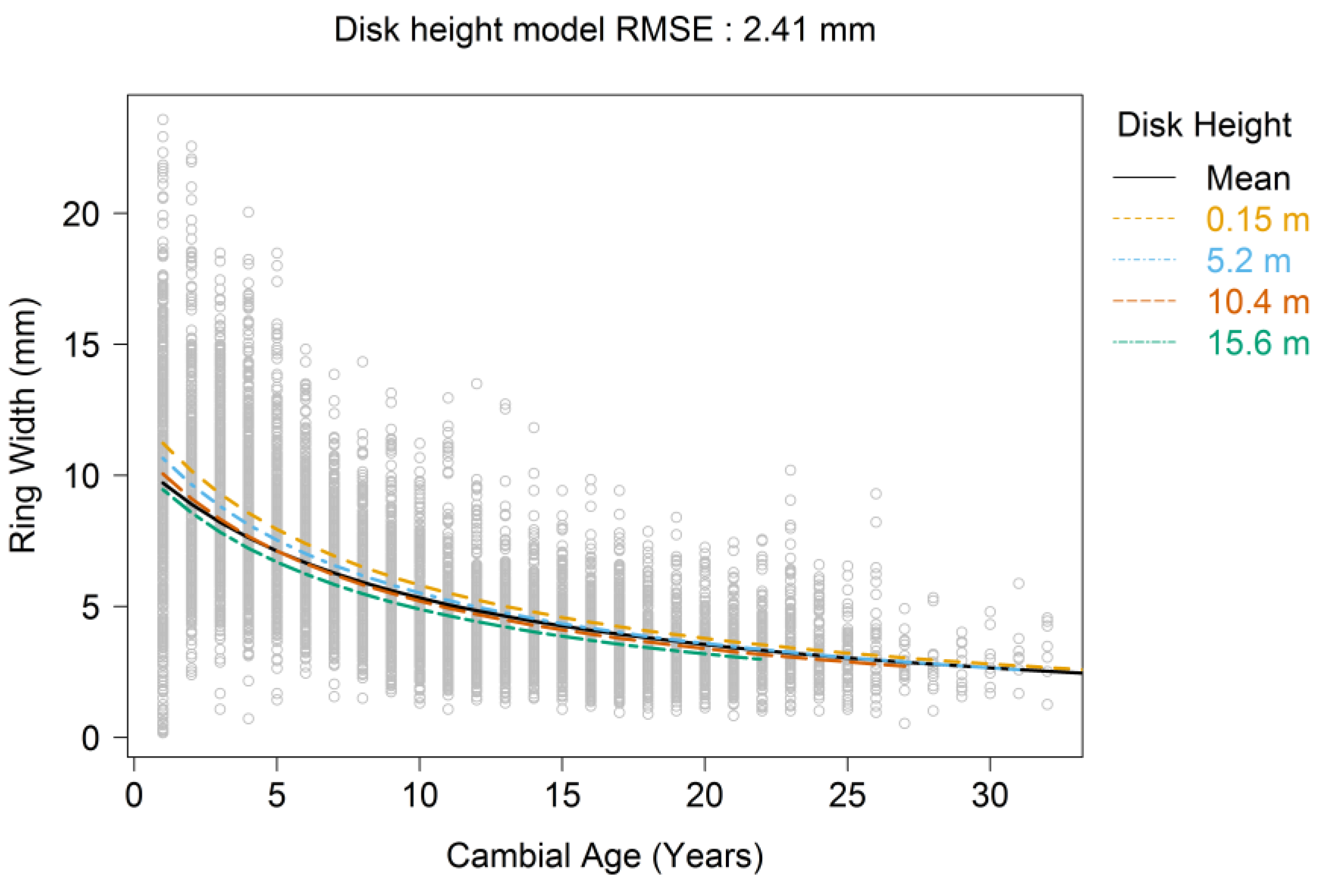
2.5. Ring Width Model Development

Unlike SG models, for which the literature provides multiple instances using the four parameters logistic function, we found very few examples to guide our choice of model form for ring width in loblolly pine. Tasissa and Burkhart [71] used a segmented linear model of ring width using data collected from image analysis. After visual exploration of the data in the current study, we focused our approach on developing a nonlinear model of annual ring width. We selected a functional form with a hyperbolic shape since it represented the observed pattern of continually decreasing ring width over time. Here, model 4 for ring width is:

$$R{W}_{ijkl}=\frac{{\beta }_0+b_{0i}+b_{0ij}}{{\beta }_1+C{A}_{ijkl}}$$

(4)

where RW_ijkl is the mean ring width (mm) in each annual growth ring, and CA_ijl is the cambial age (ring number) of the lth annual ring of the kth disk from the jth tree at the ith site. The fixed effects of the model are β₀ and β₁, where the β₀ parameter divided by the β₁ parameter represents the starting ring width at cambial age 0. The random effects for the model are b_0i and b_0ij, representing the random effect of the asymptote parameter (β₀) at the site and tree levels, respectively. To account for the butt swell that occurs in trees due to wind [72], we added a fixed effect (β₂) for the ring width term to vary by disk height, and as such model 5 is as follows:

$$R{W}_{ijkl}=\frac{{\beta }_0+b_{0i}+b_{0ij}+{\beta }_2\times D{H}_{ijkl}}{{\beta }_1+C{A}_{ijkl}}$$

(5)

where β₂ is the fixed effect to vary the β₀ parameter with disk height, DH_ijkl is the disk height (m) of the lth annual ring of the kth disk from the jth tree at the ith site, and the other parameters are the same as in ring width model 4.

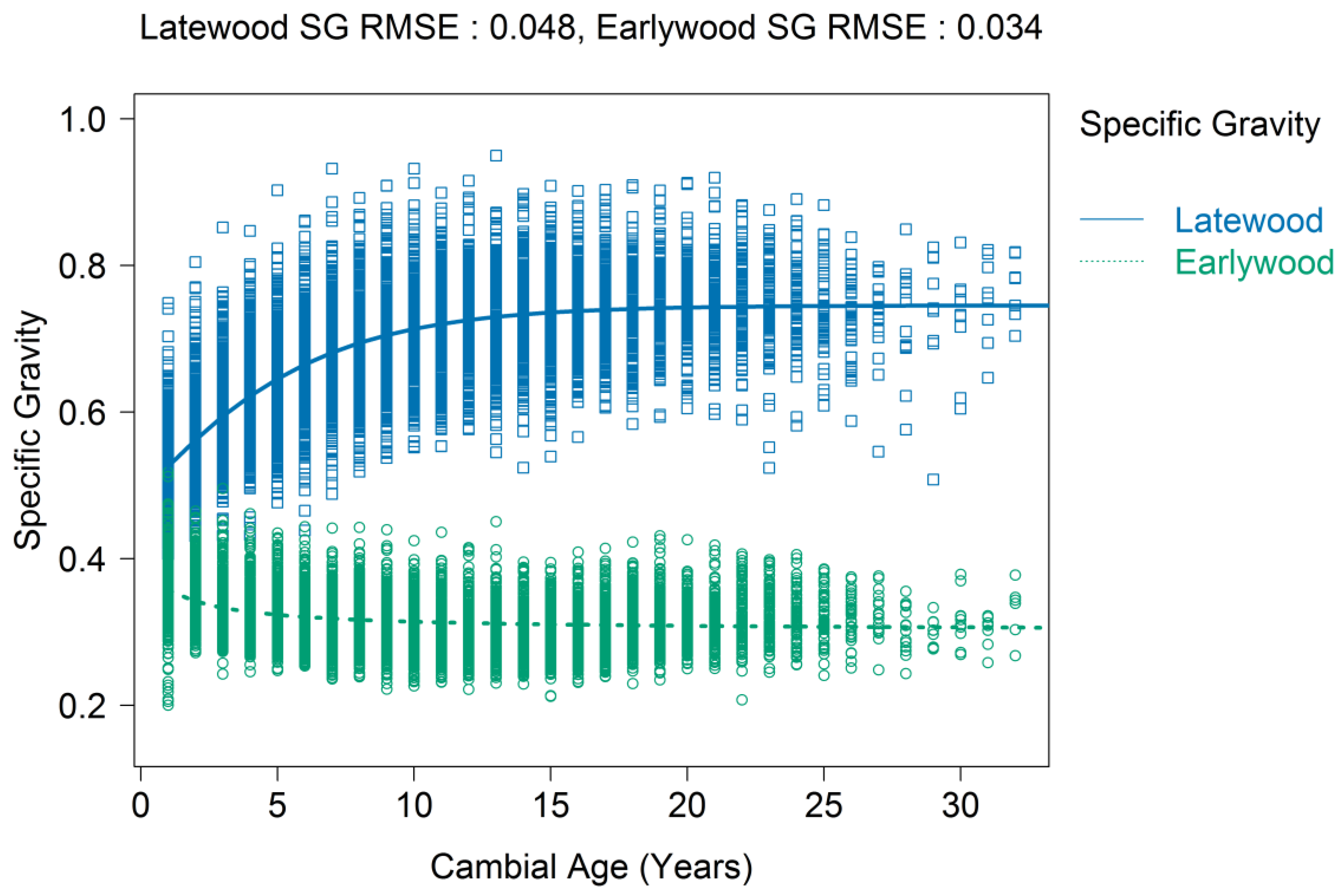
2.6. Latewood- and Earlywood-Specific Gravity Model Development

Examination of scatter plots of the data showed that latewood SG increased asymptotically with cambial age, but unlike ring SG or ring width, latewood SG had little variability with height in the stem. Modeling efforts to include height resulted in height being a non-significant term. For latewood SG the model form used was a three-parameter logistic function [68], and thus model 6 is as follows:

$$LWS{G}_{ijkl}=\frac{{\beta }_1+b_{1i}+b_{1ij}}{1+e^{\left(\frac{{\beta }_2-C{A}_{ijkl}}{{\beta }_3}\right)}}$$

(6)

where LWSG_ijkl is the mean ring latewood-specific gravity in each annual growth ring, and CA_ijkl is the cambial age (ring number) of the lth annual ring of the kth disk from the jth tree at the ith site. The fixed effects of the model are β₁, which is the asymptote as cambial age approaches infinity, β₂ is the inflection point, and β₃ is the scale parameter. The random effects for the model are b_1i and b_1ij and represent the random effect of the asymptote parameter (β₁) at the site and tree levels, respectively.

Examination of the scatter plots showed that earlywood SG was subtly influenced by cambial age, with little variation by height. For earlywood SG, the model form used was a variant on the two-parameter logistic function [68], and thus model 7 is as follows:

$$EWS{G}_{ijkl}=\left({\beta }_0+b_{0i}+b_{0ij}\right)\times e^{\frac{{\beta }_1}{C{A}_{ijkl}+{\beta }_2}}$$

(7)

where EWSG_ijkl is the mean ring latewood-specific gravity in each annual growth ring, and CA_ijkl is the cambial age (ring number) of the lth annual ring of the kth disk from the jth tree at the ith site. The fixed effects of the model are β₀, β₁, and β₂. The random effects for the model are b_0i and b_0ij, and represent the random effect of the β₀ parameter at the site and tree levels, respectively.

2.7. Latewood Percent Model Development

Because latewood percent can be expressed as a proportion that takes values on the standard unit interval (0, 1), but can also include 0 and 1, we applied zero-one-inflated beta regression to model this outcome [73]. Such mixed distributions jointly model 0 and 1 as discrete values with probabilities p₀ for 0% latewood and p₁ for 100% latewood, respectively, and continuous values on the unit interval with probability (1 − p₀ − p₁) for values between 0 and 100% latewood. Thus, the 0 and 1 values were modeled as binomial processes using logistic regression with a logit link function, while the continuous values were modeled using beta regression, also using a logit link. In this context, all three components were expressed as functions of cambial age, and were simultaneously estimated using the gamlss package. The model formulations for each component were as follows for models 8–10:

$$p_{0ijkl}=\frac{e^{{\alpha }_{0+}{\alpha }_1\times C{A}_{ijkl}}}{1+e^{{\alpha }_{0+}{\alpha }_1\times C{A}_{ijkl}}}$$

(8)

$$p_{1ijkl}=\frac{e^{{\beta }_0{}_{+}{\beta }_1\times C{A}_{ijkl}}}{1+e^{{\beta }_{0+}{\beta }_1\times C{A}_{ijkl}}}$$

(9)

$$1-p_{0ijkl}-p_{1ijkl}=\frac{e^{{\gamma }_{0+}{\gamma }_1\times C{A}_{ijkl}}}{1+e^{{\gamma }_{0+}{\gamma }_1\times C{A}_{ijkl}}}$$

(10)

where р_0ijkl is the mean probability that latewood percent is zero in each annual growth ring, р_1ijkl is the mean probability that latewood percent is 100 percent in each annual growth ring, 1 − р_0ijkl − р_1ijkl is the mean probability that latewood percent is between zero and 100% in each annual growth ring, CA_ijkl is the cambial age (ring number) of the lth annual ring of the kth disk from the jth tree at the ith site, and α₀, α₁, β₀, β₁, γ₀, γ₁ are the parameters for model 8–10. Because latewood percent varies by disk height, models 11–13 for latewood percent included the effect of disk height, with the exception of model 11 which was not significantly affected by disk height:

$$p_{0ijkl}=\frac{e^{{\alpha }_{0+}{\alpha }_1\times C{A}_{ijkl}}}{1+e^{{\alpha }_{0+}{\alpha }_1\times C{A}_{ijkl}}}$$

(11)

$$p_{1ijkl}=\frac{e^{{\beta }_0{}_{}+{\beta }_1\times C{A}_{ijkl}+{\beta }_2\times D{H}_{ijkl}}}{1+e^{{\beta }_0{}_{}+{\beta }_1\times C{A}_{ijkl}+{\beta }_2\times D{H}_{ijkl}}}$$

(12)

$$1-p_{0ijkl}-p_{1ijkl}=\frac{e^{{\gamma }_{0+}{\gamma }_1\times C{A}_{ijkl}+{\gamma }_1\times D{H}_{ijkl}}}{1+e^{{\gamma }_{0+}{\gamma }_1\times C{A}_{ijkl}+{\gamma }_1\times D{H}_{ijkl}}}$$

(13)

where DH_ijkl is the disk height (m) of the lth annual ring of the kth disk from the jth tree at the ith site, β₂ and γ₂ are new terms for the model, and the rest of the terms are the same as for models 8–10. In reality a ring would not contain 100% earlywood or latewood, however due to the use of the threshold method whereby SG is differentiated between latewood and earlywood based upon values of 0.48, as well as due to core misalignment, some rings can be designated as being all earlywood or latewood. For predicting latewood percent, we used Equations (10) and (13), respectively, for predicting the overall mean trend and the trend by disk height. To calculate fit indices and RMSE, the observed values were regressed versus the predicted values using a linear model.

2.8. Tree Map Development

Numerous publications have illustrated variation in wood properties with whole-tree maps (e.g., [38,74]). To build a tree map showing the SG variation, we predicted the height of the tree from age 1 to 30 using the dynamic model developed by Diéguez-Aranda et al. [75] for loblolly pine:

$$Y=\frac{26.14+X_0}{1+\frac{14.55}{X_0}\times t^{-1.107}}$$

(14)

where Y is the predicted height at age t, and X₀ is:

$$X_0=0.5\times (Y_0-26.14+\sqrt{{\left(Y_0-26.14\right)}^2+4\times \left(1455\times Y_0\times t_0{}^{-1.107}\right)}$$

(15)

where Y₀ is the site index (m) and t₀ is the base age (25 years). The site index we used to build the model was 26.2 m, the average site index of the stands in the study. The diameter inside bark at breast height was predicted using the ring width model developed here (Equation (5)) and the value converted from radius to diameter. In order to utilize taper models to predict the diameter at different height levels, the diameter inside bark at breast height was converted to diameter outside bark by using the relationship developed for the disks in the study:

$$\mathrm{DOB}=-0.745+1.104\times \mathrm{DIB}$$

(16)

where DOB is diameter outside bark (cm), and DIB is the diameter inside bark (cm) (R² = 0.99, RMSE = 0.58 cm). Diameters less than 10 cm (the lower range of the data) were adjusted by 1.067%, which was the mean difference between the DIB and DOB. The ring width models developed here could be used to predict the taper of the tree, however because only five or six disks were collected for each tree, the taper of the tree was not as accurately described with the model compared to a dedicated taper equation. Thus, we calculated stem taper by predicting each sequenced height level with the model generated by Bullock and Burkhart [76] for loblolly pine using their Equation (21):

$$dob=abs{\left(\frac{D^{4.1697}}{-0.9468}\right)}^{\frac{1}{4.3397}}\times abs(log{\left(1-0.8819\times \left(\frac{{\left(H-h\right)}^{2.883}}{H^{2.4610}}\right)\right)}^{\frac{1}{4.3397}}$$

(17)

where abs is the absolute value, D is the diameter at breast height in inches, H is total height in feet, and h is each sequenced height level in feet. Following the use of the taper equation the diameter at each height was converted to cm from in. The tree, DIB to DOB, and taper models provided annual height and diameter information for ages 1 to 30 throughout the entire stem. The ring width for each position was calculated by subtracting the radius at each age from the radius the previous year. We note that the taper model represents the mean trend from a range of diameters (2 to 31 cm) and heights (2.3 to 25 m), and we noticed that it produced results whereby ring width was low near the pith, increased for a number of years, and then decreased. For measured ring width we found a decrease over time. Thus, to predict the SG for the tree map we used the SG model 2 using the height level and cambial age and not the ring width. The tree map thus generated shows the yearly values of SG at each specific cambial age and height combination. In order to produce a smoothed map showing the within-tree variation in SG, the data were interpolated using an inverse-distance weighted interpolation algorithm with a 25 × 25 kernel smoother [67].

2.9. Average Tree- and Log-Specific Gravity and Proportion of Corewood throughout Rotation

The modeled annual (non-smoothed) within-tree SG variation dataset served as the basis for calculating the mean SG for the whole tree and the different logs over the rotation. In the southeastern United States, roundwood is mainly grouped into pulpwood (≥15 cm DBH), ‘chip-n-saw’ (≥20 cm and <30 cm DBH), and sawtimber (≥30 cm DBH) sized trees, with prices increasing with increasing tree size. We used these size classes as the basis for comparing the SG and relative proportions of corewood and outerwood for the whole tree and each 5.2-m log at different ages during the rotation. To calculate the average whole tree and log SG, the volume of the tree or log was calculated and then the SG at each height and cambial age combination was weighted by the volume of the ring compared to the overall volume. The weighted SG was then summed for each respective height and cambial age combination to yield the mean SG of the tree or log. The number of logs yielded at each age was dependent on whether the large end diameter (LED) of each 5.2-m log was greater than 15 cm. If the LED was less than 15 cm the material was included in the tip section, while if it was greater it was designated as a separate log.

The years at which corewood, transition wood, and outerwood were formed for ring SG followed the approach outlined by Mora et al. [69]. The first derivative of the ring SG model 2 with respect to cambial age was found:

$$\frac{d(S{G}_{ijkl})}{d(C{A}_{ijkl})}={\beta }_0+\frac{{\beta }_1+b_{1i}+b_{1ij}-{\beta }_0+{\beta }_4\times D{H}_{ijkl}}{{\beta }_4\times \left(1+e^{\left(\frac{{\beta }_2-C{A}_{ijkl}}{{\beta }_3}\right)}\right)}\times e^{\left(\frac{{\beta }_2-C{A}_{ijkl}}{{\beta }_3}\right)}$$

(18)

where the terms followed those of model 2, and d is the derivative. Corewood was assumed to be produced from the first annual ring to the age denoted by the β₂ parameter of the SG model 2, which corresponds to the age at which the maximum change in SG was reached in model 18. The production of transition wood was assumed from this point to the age at which ring SG started changing by less than 0.01, as determined by model 18. The proportion of corewood and outerwood was calculated using the same procedure described above for calculating whole tree and log SG. Briefly, each height and cambial age combination was assigned as corewood, transition wood, or outerwood. The volume of the tree or log was calculated, then the volume of corewood and outerwood at each height and cambial age combination was weighted by the volume of the ring compared to the overall volume. The weighted quantities of corewood and outerwood were then summed for each respective height and cambial age combination to yield the amount of corewood and outerwood of the tree or log, with the amount of transition wood being the difference between 100 and the combined total of corewood and outerwood. The tip section (i.e., LED < 15 cm) was assumed to be 100% corewood. An example of the segmentation between corewood, transition wood, and outerwood was done for the data measured at the stump and the first derivative of Equation (2), with the disk height being the height of the stump (0.15 m).

3. Results

The SG and ring width data varied considerably with cambial age and disk height, but this variation is typical for loblolly pine. When averaged across all rings, the mean and standard deviation (SD) for each property were as follows: ring SG: mean = 0.492, SD = 0.087; ring width: mean = 6.04 mm, SD = 3.27 mm; latewood SG: mean = 0.679, SD = 0.09; earlywood SG: mean = 0.318, SD = 0.045; and latewood percent: mean = 47%, SD = 19%. The summary tables for the model parameters are shown in

Table 2. Parameter estimates for the specific gravity and ring width models.

Property	Parameter 1	Model
		First	Second	Third
Ring SG	β0	0.355	0.377	0.414
	β1	0.643	0.611	0.630
	β2	10.71	6.40	6.30
	β3	7.28	3.81	4.45
	β4		−0.0072	−0.0076
	β5			−0.0038
Ring Width	β0	106.12	108.64
	β1	9.92	8.66
	β2		−1.108
Latewood SG	β1	0.745
	β2	−2.515
	β3	4.03
Earlywood SG	β0	0.302
	β1	0.466
	β2	1.764
Latewood Percent	α0	−2.542	−2.542
	α1	−1.967	−1.967
	β0	−4.582	−3.992
	β1	−0.0543	−0.0769
	β2		−0.0527
	γ0	−0.800	−0.271
	γ1	0.0652	0.0480
	γ2		−0.0416

¹ All model parameters significant at <0.0001. SG = specific gravity.

, and summaries of the fit indices and error statistics for the models are shown in

Table 3. Fit indices and error statics for the specific gravity and ring width fitted models.

Property	Model	AIC 1	Fit Indices (R2)			Model Errors 1
			Fixed	Site	Tree	E	RMSE	|E|%
SG	1	−25873	0.45	0.48	0.54	0.0004	0.064	10.3
	2	−26494	0.55	0.58	0.64	0.0007	0.059	9.3
	3	−26696	0.56	0.59	0.64	0.0007	0.058	9.1
Ring Width	4	30592	0.44	0.45	0.46	0.1190	2.45	29.3
	5	30477	0.46	0.46	0.47	0.1044	2.41	28.4
Latewood SG	6	−26529	0.54	0.55	0.61	0.004	0.048	7.1
Earlywood SG	7	−36462	0.16	0.17	0.30	0.0001	0.034	8.2

¹ Akaike information criterion (AIC), Mean error (E), root mean square error (RMSE), and mean absolute percentage error (|E%|) are calculated from the fixed part of each model.

, except for latewood percent since it was fit with a different method.

Ring SG increased gradually from the pith to the bark and approached an asymptote in the outerwood. For the ring SG models, the initial model (model 1) that did not include the disk height or ring width parameters explained 45% of the variation for the fixed effects and the RMSE was 0.064. Allowing ring SG to vary by height (model 2) improved the percent variation explained to 55% (fixed effects only), and reduced the RMSE to 0.059, a significant improvement over model 1 according to the AIC and a likelihood-ratio test (p < 0.0001). The intercept of model 2 (β₀) was 0.377 and the asymptote (β₁) was 0.611 (Table 2). The inclusion of the ring width term (model 3) only slightly improved the model fit (percent variation explained = 56%; RMSE = 0.058), although this model proved to be significantly better (p < 0.001) than model 2. For model 3, the intercept term (β₀) was 0.414 and the asymptote (β₁) was 0.630 (Table 2). A plot showing the variation of SG with cambial age is shown in Figure 1, with the mean trend representing model 1 and the trends by height (0.15 m, 5.2 m, 10.4 m, 15.6 m) representing predictions from model 2 at the top and bottom of each 5.2-m log.

As expected, ring width gradually decreased from pith to bark. The fixed effects of the starting model without the disk height parameter (model 4) was able to explain 44% of the variance from the fixed effects, with an RMSE of 2.45 mm. Allowing ring width to vary by height improved the fit slightly, giving 46% and 2.41 mm for the variance explained and RMSE, respectively. The AIC values were evaluated and the model proved significantly better (p < 0.001) than model 4. For model 5, the starting ring width (β₀/β₁ = 106.12 mm/9.92 mm) was 10.69 mm plus the effect of disk height. The plot of ring width by cambial age is shown in Figure 2, with the mean trend representing model 1 and the trends by height representing model 2.

Both ring SG and latewood SG had low values near the pith and approached an asymptotic value in the outerwood. However, latewood SG increased more rapidly with cambial age than ring SG, which changed more gradually. Earlywood SG showed a different trend, with a subtle decrease in SG until approximately cambial age 6, where it stabilized. For the latewood SG and earlywood SG models, only one model was constructed for each since the effect of disk height was minimal, except for the butt disk for earlywood SG, which we attribute to secondary compounds beginning to be deposited in the wood, since these samples were not extracted [56]. For latewood SG, the fixed effects of the model explained 54% of the variation in latewood SG with an RMSE of 0.0478. For earlywood SG, the fixed effects explained only 16% of the variation in the earlywood SG, and the RMSE was 0.0366. The plots of latewood SG and earlywood SG are shown in Figure 3.

Similar to ring SG and latewood SG, the latewood percent increased from the pith to the bark. Unlike the previous models developed and presented here, modeling latewood percent was significantly more challenging with regard to model convergence. The plot of latewood percent by cambial age is shown in Figure 4, with the mean trend representing models 8–10 and the trends by height representing models 11–13. Models 11–13 had a much lower AIC (−8216) than models 8–10 (−6285). Models 8–10 explained 29% of the variation, with an RMSE of 16%. Incorporating disk height into models 11–13 improved the variation explained to 46% and reduced the RMSE to 14%.

The average within-tree variation in ring SG for this study is shown in Figure 5. The map illustrates the low SG values found near the pith and the increase in SG with cambial age. The map also shows that SG decreased with height in the stem.

Table 4. Volume and specific gravity whole-tree and log values throughout the rotation.

Product Class	Age	Height (m)	DBH (cm)	Property 1	SG
					Tree	Log 1	Log 2	Log 3	Tip
Pulpwood	10	13.2	15.4	Volume (m3)	0.117	0.081	0.032	-	0.004
				Wood SG	0.471	0.484	0.445	-	0.401
				Corewood%	66	51	98	-	100
				Outerwood%	0	0	0	-	0
Chip-n-saw	15	18.4	21.2	Volume (m3)	0.305	0.169	0.091	-	0.045
				SG	0.491	0.52	0.468	-	0.426
				Corewood%	41	25	47	-	100
				Outerwood%	14	25	2	-	0
Sawtimber	27	27.4	31.1	Volume (m3)	0.967	0.403	0.258	0.168	0.138
				SG	0.514	0.557	0.515	0.476	0.428
				Corewood%	20	10	17	25	100
				Outerwood%	50	68	63	27	0
Sawtimber	30	29.2	33.0	Volume (m3)	1.157	0.461	0.3	0.202	0.194
				SG	0.516	0.562	0.522	0.482	0.431
				Corewood%	18	9	14	21	100
				Outerwood%	52	72	68	30	0

¹ Proportion of transition wood is 100 minus corewood percent minus outerwood percent. For the stem tip (large end diameter < 15 cm), the percentages of corewood was assumed to be 100%.

shows the average tree and log specific gravity for the different product classes at the age the tree first reached the size required for a specific product class, and at age 30. The tree reached the pulpwood size (>15 cm DBH) at age 10, the chip-n-saw size (≥20 cm and <30 cm DBH) at age 15, and the sawtimber size (≥30 cm DBH) size at age 27. At the pulpwood (age 10) and chip-n-saw (age 15) sizes, the trees would yield two 5.2-m logs, and as the tree approached the sawtimber (age 27) size and maturity (age 30), the trees yielded three 5.2-m logs. Whole tree SG increased subtly from 0.471 at age 10 to 0.491 at age 15, then to 0.514 at age 27, and finally to 0.516 at age 30. The SG for the first log however increased from 0.484 at age 10 to 0.52 at age 15, 0.557 at age 27, and 0.562 at age 30. At age 10, the proportion of corewood was high and the proportion of outerwood low, with whole tree proportions of 66 and 0% for corewood and outerwood, respectively. At age 15 the corewood proportion had decreased to 41% and the outerwood to 14%, with transition wood as the remaining proportion. By age 27 the corewood proportion was 20% while outerwood was 50%, and by age 30 the corewood proportion was 18% and outerwood 52%. An example of the segmentation between corewood, transition wood, and outerwood for the data measured at the stump and the first derivative of Equation (2), with the disk height being the height of the stump (0.15 m) is shown in Figure 6.

4. Discussion

The radial and longitudinal (i.e., at different tree heights) variations of SG in this study are consistent with previous studies on loblolly pine from plantations [69,70,77,78]. The within-tree variation in SG was captured in a model that predicted SG values against cambial age (Figure 1), while incorporating disk height in the model gave a better fit and showed that predicted values decreased with height in the tree. The modeling approach we used here did not address the timing of silvicultural treatments in the rotation because even though they did vary between stands, the silvicultural prescriptions were very similar. Including the effects of silviculture may have improved the model fit at the expense of model complexity. Antony et al. [78] modeled latewood SG and showed that latewood SG decreased with increasing fertilization intensity. Included in their paper is a plot of mean latewood SG with the x-axis in years instead of cambial age to illustrate the decreasing trend. This approach has the benefit that the effects of silvicultural treatment are displayed at a consistent time point. However, their modeling efforts were focused on cambial age, as done in this paper, but with the added terms of timing of treatment and years since treatment.

The generation of a stem map showing the within-tree variation of SG illustrates the differences in ring SG between juvenile corewood and outerwood, and mature corewood and outerwood [10]. Similar SG maps have been generated for loblolly pine [74] and Scots pine [38]; however, the SG map in the present study shows a greater longitudinal variation in the region ascribed to corewood. Indeed, this shows some resemblance to Kibblewhite’s [79] schematic for mature corewood as a zone of wood with properties from pith to bark that differed from the juvenile corewood and juvenile outerwood found lower in the tree. Note that similar wood density maps have been generated for other conifer genera (Abies, Picea, Pseudotsuga), and while they show some longitudinal variability, they do not have the same general pattern of decreasing corewood density from the base to the top of the tree [80,81].

While nearly all wood properties vary with cambial age, we found that only SG and latewood percent varied significantly by disk height. Ring width had subtle variations with height, likely influenced by the swell that occurs at the base of the stem [72]. Since differences with disk height were not observed for latewood or earlywood SG, we attribute the changes in SG by height to a corresponding decrease in latewood percent with height in the tree. The model integrating ring width did not provide a large improvement over the model with only cambial age and disk height as explanatory variables. The stands sampled here were located fairly close to each other and had similar silvicultural treatments. It is likely that the growth rates were also similar, thus the effect of ring width was likely lower than if the stands had received very different silvicultural treatments, or were from different geographical regions (see Jordan et al. [77]).

Like other studies that modeled loblolly pine ring SG, we used the same four-parameter logistic model, but found subtle differences in the model parameters. Specifically, Mora et al. [69], examining samples collected from breast height (1.37 m), found a lower intercept value (β₀) of 0.265 compared to 0.377 in the current study, determined with the model incorporating disk height. Their asymptote value (β₁) of 0.573 was lower than our corresponding value of 0.601 (i.e., 0.611 + 1.37 × −0.0072). The difference between these values may be due in part to stand age; here we sampled tree ages from 24 to 33, while Mora et al. [69] sampled 21- and 22-year-old trees. The inflection point (β₂) and scale parameters (β₃) were also quite different, which may be attributed to the difference in sampling heights between the studies. Whereas here we sampled disks located between 5.2-m logs used in a lumber study, Mora et al. [69] sampled only at breast height. Antony et al. [70] also utilized the four-parameter logistic model for loblolly pine, but used the information mainly to estimate the relative proportions of corewood and outerwood.

The model that proved most problematic to fit was the latewood percent model. This was attributed to the high variability in the data, particularly to the occurrence of rings with either 0 or 100% latewood, which are mainly an artifact of limitations in both densitometer resolution and the threshold method for assigning latewood. Specific to the latter, latewood percent is not a measurement per se, but rather an arbitrary classification based on the width of the latewood as a proportion of total ring width. In a given ring, SG values above 0.48 were assigned to the latewood. Since loblolly pine has abrupt earlywood to latewood transitions, the threshold method works well for most rings, but can present some challenges in rings near the pith [55]. Spruces (e.g., Picea mariana, Picea abies (L.) H. Karst.) and some other pines have gradual transitions between earlywood and latewood, and benefit from different approaches for assigning latewood, such as the use of polynomial models to identify the within-ring inflection point of SG as the demarcation between earlywood and latewood [82]. For loblolly pine, Eberhardt and Samuelson [56] found little difference between the threshold method and polynomial models. Misaligned rings can also influence latewood percent when the threshold method is used. This is because the X-ray densitometer used in this study scans a relatively small vertical window (~1.6 mm) at each radial step (0.06 mm). If both low and high density wood is present in the vertical scan window due to misalignment, some rings may not have SG values below the designated threshold. The SilviScan system can correct for some of these curved ring problems, but not all of them [26]. Jacquin et al. [20] are testing an alternative method for handling sample tilt in densitometry. While the distinction between earlywood and latewood SG is important for latewood percent calculations, it makes little difference with regard to calculating ring SG [56].

Trees harvested during a thinning operation at mid-rotation and sold as pulpwood have lower whole-tree and log SG values than older trees sold as either chip-n-saw or sawtimber material; however, few studies on loblolly pine, or the other southern pines, have addressed the usefulness of ring SG models at harvest times throughout a rotation, or used this information to determine whole-tree or log SG values as in the present study (Table 4). Jordan et al. [77] constructed region-wide maps showing the variation of whole-core SG values at three ages from samples collected at breast height for loblolly pine throughout the southern United States. Antony et al. [83] constructed similar region-wide maps showing the variation in SG by height using data collected from whole disks. Mora and Schimleck [74] compared three techniques for constructing within-tree wood properties maps using loblolly pine data derived from near-infrared spectroscopy calibration models and SilviScan. For determining the transition ages between corewood and outerwood, Clark III et al. [16] used a different methodology than the first derivative approach used here, whereby segmented polynomials and threshold values were used to assign the transition, although Mora et al. [69] and Antony et al. [70] both used the latter approach. In all three studies, only breast height samples were analyzed and thus whole-tree and whole-log values were not described. In Scots pine, Auty et al. [38] modeled radial and longitudinal variation in wood density and simulated wood density values and proportion of corewood for different combinations of thinning regimes and rotation lengths.

Not addressed in the current study are models related to other wood properties, such as MFA, tracheid length, and cell wall thickness, among others. The influence of silviculture on these properties can often be very different than for SG [46]. For example, Clark et al. [16] found that outerwood designated using SG was produced at approximately half the age than when designated using MFA. Accordingly, as with latewood percent being dependent on how it is designated, the amount of corewood is dependent on the physical property used and its corresponding threshold.

In this study we linked numerous models together to construct the within-tree SG map and the table showing SG values over a rotation at the tree and log level. Chaining models together can cause problems, including recursive errors in the model system. While not addressed in this study, future work will focus on simultaneous estimation of ring-level wood properties models to create a framework for scaling up predictions to the tree, stand and regional levels.

5. Conclusions

In this study, we measured SG and ring width using X-ray densitometry for loblolly pine obtained from intensively managed plantations. Non-linear mixed-effects models were constructed to quantify the variation in these properties that occur within the trees. The change from corewood to outerwood is related to increasing cambial age, while the transition from juvenile to mature wood is related to height within the tree. The fixed effects of the models were able to explain 56, 46, 54, 16, and 46 percent of the within-tree variation for ring SG, ring width, latewood SG, earlywood SG, and latewood percent, respectively. A two-dimensional tree map was constructed which showed changes in tree and log SG values and the proportion of corewood over time. Whole-tree SG increased from 0.471 at age 10 to 0.516 at age 30, with the proportion of corewood decreasing from 66% to 52% over the same time period. For the first log, the changes with age were more pronounced, with SG increasing from 0.484 at age 10 to 0.562 at age 30, with the proportion of corewood decreasing from 51% to 9%. Developing systems of models is an important step in integrating wood properties into forest growth and yield systems.

References

1. Sedjo, R.A. The role of forest plantations in the world’s future timber supply. For. Chron. 2001, 77, 221–225. [Google Scholar] [CrossRef]
2. Sedjo, R.A. The potential of high-yield plantation forestry for meeting timber needs. New For. 1999, 17, 339–359. [Google Scholar] [CrossRef]
3. FAO. Global Forest Resources Assessment 2005, Main Report. Progress towards Sustainable Forest Management; FAO Forestry Paper 147; FAO: Rome, Italy, 2006. [Google Scholar]
4. Wear, D.N.; Greis, J.G. Southern Forest Resource Assessment: Summary of Findings. J. For. 2002, 100, 6–14. [Google Scholar]
5. McKeand, S.; Mullin, T.; Bryam, T.; White, T. Deployment of genetically improved loblolly and slash pines in the South. J. For. 2003, 101, 32–37. [Google Scholar]
6. Borders, B.E.; Bailey, R.L. Loblolly pine—Pushing the limits of growth. South. J. Appl. For. 2001, 25, 69–74. [Google Scholar]
7. Fox, T.R.; Jokela, E.J.; Allen, H.L. The development of pine plantation silviculture in the southern United States. J. For. 2007, 105, 337–347. [Google Scholar]
8. Zhao, D.; Kane, M.B.; Teskey, R.O.; Fox, T.R.; Albaugh, T.J.; Allen, H.L.; Rubilar, R.A. Maximum response of loblolly pine plantations to silvicultural management in the southern United States. For. Ecol. Manag. 2016, 375, 105–111. [Google Scholar] [CrossRef]
9. Clark, A., III; Jordan, L.; Schimleck, L.; Daniels, R.F. Effect of initial planting spacing on wood properties of unthinned loblolly pine at age 21. For. Prod. J. 2008, 58, 78–83. [Google Scholar]
10. Burdon, R.D.; Kibblewhite, R.P.; Walker, J.C.F.; Megraw, R.A.; Evans, R.; Cown, D.J. Juvenile versus mature wood: A new concept, orthogonal to corewood versus outerwood, with special reference to Pinus radiata and P-taeda. For. Sci. 2004, 50, 399–415. [Google Scholar]
11. Moore, J.R.; Cown, D.J. Corewood (juvenile wood) and its impact on wood utilisation. Curr. For. Rep. 2017, 3, 107–119. [Google Scholar] [CrossRef]
12. Lachenbruch, B.; Moore, J.R.; Evans, R. Radial variation in wood structure and function in woody plants, and hypotheses for its occurrence. In Size- and Age-Related Changes in Tree Structure and Function; Meinzer, F.C., Lachenbruch, B., Dawson, T.E., Eds.; Springer: Berlin, Germany, 2011; pp. 121–164. [Google Scholar]
13. Larson, P.R.; Kretschmann, D.E.; Clark, A., III; Isebrands, J.G. Formation and Properties of Juvenile Wood in Southern Pines; FPL-TR-129; US for Serv. Forest Products Laboratory: Madison, WI, USA, 2001. [Google Scholar]
14. Ying, L.; Kretschmann, D.E.; Bendtsen, B.A. Longitudinal shrinkage in fast-grown loblolly pine wood. For. Prod. J. 1994, 44, 58–62. [Google Scholar]
15. Jordan, L.; He, R.; Hall, D.B.; Clark, A., III; Daniels, R.F. Variation in loblolly pine ring microfibril angle in the Southeastern United States. Wood Fiber Sci. 2007, 39, 352–363. [Google Scholar]
16. Clark, A., III; Daniels, R.F.; Jordan, L. Juvenile/mature wood transition in loblolly pine as defined by annual ring specific gravity, proportion of latewood, and microfibril angle. Wood Fiber Sci. 2006, 38, 292–299. [Google Scholar]
17. Butler, A.; Dahlen, J.; Daniels, R.F.; Eberhardt, T.L.; Antony, F. Bending strength and stiffness of loblolly pine lumber from intensively managed stands located on the Georgia Lower Coastal Plain. Eur. J. Wood Prod. 2016, 47, 91–100. [Google Scholar] [CrossRef]
18. Hoag, M.; McKimmy, M.D. Direct scanning X-ray densitometry of thin wood sections. For. Prod. J. 1988, 38, 23–26. [Google Scholar]
19. Xiang, W.; Leitch, M.; Auty, D.; Duchateau, E.; Achim, A. Radial trends in black spruce wood density can show an age- and growth-related decline. Ann. For. Sci. 2014, 71, 603–615. [Google Scholar] [CrossRef]
20. Jacquin, P.; Longuetaud, F.; Leban, J.M.; Mothe, F. X-ray microdensitometry of wood: A review of existing principles and devices. Dendrochronologia 2017, 42, 42–50. [Google Scholar] [CrossRef]
21. Evans, R.; Stuart, S.A.; Van Der Touw, J. Microfibril angle scanning of increment cores by X-ray diffractometry. Appita J. 1996, 6, 411–414. [Google Scholar]
22. Evans, R.; Hughes, M.; Menz, D. Microfibril angle variation by scanning X-ray diffractometry. Appita J. 1999, 5, 363–367. [Google Scholar]
23. Donaldson, L.L. Microfibril angle: Measurement, variation and relationships—A review. IAWA J. 2008, 4, 345–386. [Google Scholar] [CrossRef]
24. Hirn, U.; Bauer, W. A review of image analysis based methods to evaluate fiber properties. Lenzing. Ber. 2006, 86, 96–105. [Google Scholar]
25. Chen, Z.Q.; Karlsson, B.; Mӧrling, T.; Olsson, L.; Mellerowicz, E.J.; Wu, H.X.; Lundqvist, S.O.; Gil, M.R.G. Genetic analysis of fiber dimensions and their correlation with stem diameter and solid-wood properties in Norway spruce. Tree Genet. Genomes 2016, 12, 123. [Google Scholar] [CrossRef]
26. Evans, R. Rapid measurement of the transverse dimensions of tracheids in radial wood sections from Pinus radiata. Holzforschung 1994, 48, 168–172. [Google Scholar] [CrossRef]
27. Chen, F.; Evans, R. A robust approach for vessel identification and quantification in eucalypt pulpwoods. IAWA J. 2005, 6, 442–447. [Google Scholar]
28. Vahey, D.W.; Zhu, J.Y.; Scott, C.T. Wood density and anatomical properties in suppressed-growth trees: Comparison of two methods. Wood Fiber Sci. 2007, 39, 462–471. [Google Scholar]
29. So, C.L.; Via, B.K.; Groom, L.H.; Schimleck, L.R.; Shupe, T.F.; Kelley, S.S.; Rials, T.G. Near infrared spectroscopy in the forest products industry. For. Prod. J. 2004, 54, 7–16. [Google Scholar]
30. Tsuchikawa, S.; Kobori, H. A review of recent application of near infrared spectroscopy to wood science and technology. J. Wood Sci. 2015, 61, 213–220. [Google Scholar] [CrossRef]
31. Nabavi, M.; Dahlen, J.; Schimleck, L.; Eberhardt, T.L.; Montes, C. Regional calibration models for predicting loblolly pine tracheid properties using near-infrared spectroscopy. Wood Sci. Technol. 2018, 52, 445–463. [Google Scholar] [CrossRef]
32. Huang, C.-L.; Lindström, H.; Nakada, R.; Ralston, J. Cell wall structure and wood properties determined by acoustics—A selective review. Holz Roh Werkstoff 2003, 61, 321–335. [Google Scholar] [CrossRef]
33. Mason, E.G.; Hayes, M.; Pink, N. Validation of ultrasonic velocity estimates of wood properties in discs of radiata pine. N. Z. J. For. Sci. 2017, 47, 16. [Google Scholar] [CrossRef]
34. Hasegawa, M.; Takata, M.; Matsumura, J.; Oda, K. Effect of wood properties on within-tree variation in ultrasonic wave velocity in softwood. Ultrasonics 2010, 51, 296–302. [Google Scholar] [CrossRef] [PubMed]
35. Hasegawa, M.; Mori, M.; Matsumura, J. Relations of fiber length to within-tree variation of ultrasonic wave velocity in fast-growing trees. Wood Fiber Sci. 2015, 3, 1–6. [Google Scholar]
36. Riddell, M.; Cown, D.; Harrington, J.; Lee, J.; Moore, J. Assessing spiral grain angle by light transmission—Proof of concept. IAWA J. 2012, 33, 1–14. [Google Scholar] [CrossRef]
37. Moore, J.R.; Cown, D.J.; McKinley, R.B. Modelling spiral grain angle variation in New Zealand-grown radiata pine. N. Z. J. For. Sci. 2015, 45, 15. [Google Scholar] [CrossRef]
38. Auty, D.; Achim, A.; Macdonald, E.; Cameron, A.D.; Gardiner, B.A. Models for predicting wood density variation in Scots pine. Forestry 2014, 87, 449–458. [Google Scholar] [CrossRef]
39. Kimberley, M.O.; Cown, D.J.; McKinley, R.B.; Moore, J.R.; Dowling, L.J. Modelling the variation in wood density within and among trees in stands of New Zealand-grown radiata pine. N. Z. J. For. Sci. 2015, 45, 22. [Google Scholar] [CrossRef]
40. McLean, J.P.; Moore, J.R.; Gardiner, B.A.; Lee, S.J.; Mochan, S.J.; Jarvis, M.C. Variation of radial wood properties from genetically improved Sitka spruce growing in the UK. Forestry 2016, 89, 109–116. [Google Scholar] [CrossRef]
41. Kimberley, M.O.; McKinley, R.B.; Cown, D.J.; Moore, J.R. Modelling the variation in wood density of New Zealand-grown Douglas-fir. N. Z. J. For. Sci. 2017, 47, 15. [Google Scholar] [CrossRef]
42. Megraw, R.A. Wood Quality Factors in Loblolly Pine; TAPPI: Peachtree Corners, GA, USA, 1985; p. 88. [Google Scholar]
43. Downes, G.M.; Drew, D.; Battaglia, M.; Schulze, D. Measuring and modelling stem growth and wood formation: An overview. Dendrochronologia 2009, 27, 147–157. [Google Scholar] [CrossRef]
44. Briggs, D.G. Enhancing forest value productivity through fiber quality. J. For. 2010, 108, 174–182. [Google Scholar]
45. Burkhart, H.E.; Tomé, M. Modeling Forest Trees and Stands; Springer: Berlin, Germany, 2012; pp. 405–427. ISBN 978-90-481-3170-9. [Google Scholar]
46. Antony, F.; Jordan, L.; Schimleck, L.R.; Daniels, R.F.; Clark, A., III. The effect of mid-rotation fertilization on the wood properties of loblolly pine (Pinus taeda). IAWA J. 2009, 30, 49–58. [Google Scholar] [CrossRef]
47. Love-Myers, K.R.; Clark, A., III; Schimleck, L.; Jokela, E.J.; Daniels, R.F. Specific gravity responses of slash pine and loblolly pine following mid-rotation fertilization. For. Ecol. Manag. 2009, 257, 2342–2349. [Google Scholar] [CrossRef]
48. Love-Myers, K.R.; Clark, A., III; Schimleck, L.R.; Dougherty, P.M.; Daniels, R.F. The effects of irrigation and fertilization on specific gravity of loblolly pine. For. Sci. 2010, 56, 484–493. [Google Scholar]
49. Clark, A., III; Borders, B.E.; Daniels, R.F. Impact of vegetation control and annual fertilization on properties of loblolly pine wood at age 12. For. Prod. J. 2004, 54, 90–96. [Google Scholar]
50. Antony, F.; Schimleck, L.R.; Jordan, L.; Hornsby, B.; Dahlen, J.; Daniels, R.F.; Clark, A., III; Apiolaza, L.A.; Huber, D. Growth and wood properties of genetically improved loblolly pine: Propagation type comparison and genetic parameters. Can. J. For. Res. 2014, 44, 263–272. [Google Scholar] [CrossRef]
51. Filipescu, C.N.; Stoehr, M.U.; Pigott, D.R. Variation of lumber properties in genetically improved full-sib families of Douglas-fir in British Columbia, Canada. Forestry 2018, 91, 320–326. [Google Scholar] [CrossRef]
52. Butler, A.; Dahlen, J.; Eberhardt, T.L.; Montes, C.; Antony, F.; Daniels, R.F. Acoustic evaluation of loblolly pine tree- and lumber-length logs allows for segregation of lumber modulus of elasticity, not for modulus of rupture. Ann. For. Sci. 2017, 74, 20. [Google Scholar] [CrossRef]
53. Dahlen, J.; Montes, C.; Eberhardt, T.L.; Auty, D. Probability models that relate nondestructive test methods to lumber design values of plantation loblolly pine. Forestry 2018, 91, 295–306. [Google Scholar] [CrossRef]
54. ASTM International. ASTM D2395–17: Standard Test Methods for Density and Specific Gravity (Relative Density) of Wood and Wood-Based Materials; ASTM International: West Conshohocken, PA, USA, 2017. [Google Scholar]
55. Antony, F.; Schimleck, L.R.; Daniels, R.F. A comparison of earlywood-latewood demarcation methods—A case study in loblolly pine. IAWA J. 2012, 33, 187–195. [Google Scholar]
56. Eberhardt, T.L.; Samuelson, L.J. Collection of wood quality data by X-ray densitometry: A case study with three southern pines. Wood Sci. Technol. 2015, 49, 739–753. [Google Scholar] [CrossRef]
57. R Core Team. R: A Language and Environment for Statistical Computing. R Foundation for Statistical Computing, Vienna, Austria. 2018. Available online: http://www.R-project.org/ (accessed on 18 April 2018).
58. RStudio. RStudio: Integrated Development Environment for R. Boston, MA. 2018. Available online: https://www.rstudio.com/ (accessed on 18 April 2018).
59. Wickham, H.; Francois, R. dplyr: A Grammar of Data Manipulation. 2017. R Package Version 0.7.4. Available online: https://CRAN.R-project.org/package=dplyr (accessed on 18 April 2018).
60. Rigby, R.A.; Stasinopoulos, D.M. Generalized additive models for location, scale and shape, (with discussion). Appl. Stat. 2005, 54, 507–554. [Google Scholar] [CrossRef]
61. Wickham, H. ggplot2: Elegant Graphics for Data Analysis; Springer: New York, NY, USA, 2009; p. 212. [Google Scholar]
62. Auguie, B. gridExtra: Miscellaneous Functions for “Grid” Graphics. 2016. R Package Version 2.2.1. Available online: https://CRAN.R-project.org/package=gridExtra (accessed on 18 April 2018).
63. Pebesma, E.J. Multivariable geostatistics in S: The gstat package. Comput. Geosci. 2004, 30, 683–691. [Google Scholar] [CrossRef]
64. Gräler, B.; Pebesma, E.; Heuvelink, G. Spatio-temporal interpolation using gstat. R J. 2016, 8, 204–218. [Google Scholar]
65. Pinheiro, J.; Bates, D.; DebRoy, S.; Sarkar, D.; R Core Team. nlme: Linear and Nonlinear Mixed Effects Models. 2016. R Package Version 3.1–128. Available online: https://CRAN.R-project.org/package=nlme (accessed on 18 April 2018).
66. Hijmans, R.J. Raster: Geographic Data Analysis and Modeling. 2016. R Package Version 2.5–8. Available online: https://CRAN.R-project.org/package=raster (accessed on 18 April 2018).
67. Baddeley, A.; Rubak, E.; Turner, R. Spatial Point Patterns: Methodology and Applications with R; Chapman and Hall/CRC Press: London, UK, 2016; p. 810. ISBN 9781482210200. [Google Scholar]
68. Ratkowsky, D.A. Handbook of Nonlinear Regression Models; Marcel Dekker: New York, NY, USA, 1990; p. 241. [Google Scholar]
69. Mora, C.R.; Allen, H.L.; Daniels, R.F.; Clark, A., III. Modeling corewood-outerwood transition in loblolly pine using wood specific gravity. Can. J. For. Res. 2007, 37, 999–1011. [Google Scholar] [CrossRef]
70. Antony, F.; Schimleck, L.R.; Jordan, L.; Clark, A., III; Daniels, R.F. Effect of early age woody and herbaceous competition control on wood properties of loblolly pine. For. Ecol. Manag. 2011, 262, 1639–1647. [Google Scholar] [CrossRef]
71. Tasissa, G.; Burkhardt, H.E. Modeling thinning effects on ring width distribution in loblolly pine (Pinus taeda). Can. J. For. Res. 1997, 27, 1291–1301. [Google Scholar] [CrossRef]
72. Gardiner, B.; Berry, P.; Moulia, B. Review: Wind impacts on plant growth, mechanics and damage. Plant Sci. 2016, 245, 94–118. [Google Scholar] [CrossRef] [PubMed]
73. Ospina, R.; Ferrari, S.L. A general class of zero-or-one inflated beta regression models. Comput. Stat. Data Anal. 2012, 56, 1609–1623. [Google Scholar] [CrossRef]
74. Mora, C.R.; Schimleck, L.R. Determination of within-tree variation of Pinus taeda wood properties by near infrared spectroscopy. Part 2: Whole-tree wood property maps. Appita 2009, 62, 232–238. [Google Scholar]
75. Diéguez-Aranda, U.; Burkhardt, H.E.; Amateis, R.L. Dynamic site model for loblolly pine (Pinus taeda L.) plantations in the United States. For. Sci. 2006, 52, 262–272. [Google Scholar]
76. Bullock, B.P.; Burkhart, H.E. Equations for predicting green weight of loblolly pine trees in the south. South. J. Appl. For. 2001, 27, 153–159. [Google Scholar]
77. Jordan, L.; Clark, A., III; Schimleck, L.R.; Hall, D.; Daniels, R.F. Regional variation in wood specific gravity of planted loblolly pine in the United States. Can. J. For. Res. 2008, 38, 698–710. [Google Scholar] [CrossRef]
78. Antony, F.; Schimleck, L.R.; Hall, D.B.; Clark, A., III; Daniels, R.F. Modeling the effect of midrotation fertilization on specific gravity of loblolly pine (Pinus taeda L.). For. Sci. 2011, 57, 145–152. [Google Scholar]
79. Kibblewhite, R.P. Designer fibres for improved papers through exploiting variations in wood microstructure. Appita J. 1999, 52, 429–435,440. [Google Scholar]
80. MacDonald, E.; Gardiner, B.; Mason, W. The effects of transformation of even-aged stands to continuous cover forestry on conifer log quality and wood properties in the UK. Forestry 2009, 83, 1–16. [Google Scholar] [CrossRef]
81. Longuetaud, F.; Mothe, F.; Fournier, M.; Dlouha, H.; Santenoise, P.; Deleuze, C. Within-stem maps of wood density and water content for characterization of species: A case study on three hardwood and two softwood species. Ann. For. Sci. 2016, 73, 601–614. [Google Scholar] [CrossRef]
82. Koubaa, A.; Tony Zhang, S.Y.; Makni, S. Defining the transition from earlywood to latewood in black spruce based on intra-ring wood density profiles from X-ray densitometry. Ann. For. Sci. 2002, 59, 511–518. [Google Scholar] [CrossRef]
83. Antony, F.; Schimleck, L.R.; Daniels, R.F.; Clark, A., III; Hall, D.B. Modeling the longitudinal variation in wood specific gravity of planted loblolly pine (Pinus taeda) in the United States. Can. J. For. Res. 2010, 40, 2439–2451. [Google Scholar] [CrossRef]
Figure 1. Variation in mean specific gravity with cambial age predicted for the overall data using model 1 and for different height levels using model 2 with the root mean square error (RMSE) for model 2 listed. Open gray circles represent the observed specific gravity (SG) values.
Forests 09 00292 g001
Figure 2. Ring width (mm) predicted for overall data using model 4 and for different height levels using model 5 with the RMSE for model 5 listed. Open gray circles represent the observed ring width values.
Forests 09 00292 g002
Figure 3. Latewood-specific gravity and earlywood-specific gravity predicted for overall data with RMSE for models 6 and 7 listed.
Forests 09 00292 g003
Figure 4. Latewood percent versus cambial age. The mean predicted values for the overall data were generated using model 10, and those for different height levels using model 13 with the RMSE for model 13 listed. Open gray circles represent the observed latewood percent values.
Forests 09 00292 g004
Figure 5. Map of average within-tree variation of specific gravity (SG) in this study, smoothed using inverse-distance weighted interpolation.
Forests 09 00292 g005
Figure 6. Segmentation between corewood (<6.4 years), transition wood (6.4 to 12.4 years), and outerwood (>12.4 years) for the ring SG stump (0.15 m) data and the modeled response.
Forests 09 00292 g006