Automatic Detection of Single Trees in Airborne Laser Scanning Data through Gradient Orientation Clustering

Abstract

Currently, existing methods for single-tree detection based on airborne laser scanning (ALS) data usually require some thresholds and parameters to be set manually. Manually setting threshold or parameters is laborious and time-consuming, and for dense forests, the high commission and omission rate make most existing single-tree detection techniques inefficient. As a solution to these problems, this paper proposed an automatic single-tree detection method in ALS data through gradient orientation clustering (GOC). In this method, the rasterized Canopy Height Model (CHM) was derived from ALS data using surface interpolation. Then, potential trees were assumed as approximate conical shapes and extracted based on the GOC. Finally, trees were identified from the potential trees based on the compactness of the crown shape. This method used the gradient orientation information of rasterized CHM, thus increasing the generalization of single-tree detection method. In order to verify the validity and practicability of the proposed method, twelve 1256 m² circular study plots of different forest types were selected from the benchmark dataset (NEWFOR), and the results from nine different methods were presented and compared for these study plots. Among nine methods, the proposed method had the highest root mean square matching score (RMS_M = 43). Moreover, the proposed method had excellent detection (M > 47) in both single-layer coniferous and single-layered mixed stands.

1. Introduction

Remote sensing (RS) is a synthesized, efficient, and rapid means of obtaining earth surface information, which can help forestry management departments achieve high-precision forest resource surveys, timber production estimation, and other applications [1,2,3]. Light detection and ranging (LiDAR) is an RS method that uses light in the form of a pulsed laser to measure ranges (i.e., variable distances) to the Earth. These light pulses, combined with other data recorded by the airborne system, generate precise, three-dimensional information about the shape of the Earth and its surface characteristics. Airborne laser scanning (ALS) is a widely used LiDAR technology in forestry, which has a unique advantage in 3D terrain and forest height detection. It can quickly and accurately obtain a digital surface model (DSM) and forest height information for forested land [4,5]. According to the statistics, single-tree detection algorithms that use active RS data, such as ALS, have grown rapidly in recent years, accounting for 80% of the total increase in RS area, at the same time, those algorithms using passive data or a fusion of passive and active data accounts for 8% and 12% respectively [6]. To date, there are many methods for single-tree detection based on ALS data acquired for forest mapping, precision forestry management, and forest timber evaluation [7,8,9,10,11,12].

Currently, some researchers have proposed automatic or semi-automatic single-tree detection methods. According to the data processing, the single-tree detection method based on ALS data can be divided into three categories: (1) raster-based methods; (2) point cloud-based methods; and (3) methods combing raster, point cloud, and a prior information [13]. Our research focuses on the raster-based method which is based on rasterized canopy height model (CHM). This type of method needs to rasterize the point cloud data and detect single trees in the rasterized data. In this method, height normalised ALS points are classified into ground points and above-ground points. Then, the points are rasterised to produce a digital terrain model (DTM, ground points only) and digital surface model (DSM, maximum of all points) by following the generation of a triangulated irregular network. As a result, the CHM was built based on the DTM and the DSM. For example, Hyyppa et al. [14] firstly used high-pulse-rate laser scanners to extract the information at tree level and accurate 3D tree height maps, which is used for forest inventories at stand level. This method calculated the stem volume and basal area for each tree by using the tree height and crown boundary information obtained with the laser scanner for each individual tree. The precision obtained by the new method is better than that in conventional standwise forest inventories. Persson et al. [15] generated digital canopy model with different scales to estimate the height and crown diameter of identified trees by using a parabolic surface. This study demonstrates the usefulness of airborne laser scanning data for detecting and measuring individual trees. Popescu et al. [16] proposed a Local Maximum (LM) technique with a variable window size, which is demonstrated more appropriate than the static LM filter or the grid approach that arbitrarily selects only the highest values in a grid with a user defined size. But, this study was based on rather limited samples with no stratification based on tree species or ages. The LiDAR data were not fully exploited by neglecting secondary returns from within the tree canopy. Chen et al. [17] proposed a marker-controlled watershed segmentation for LiDAR CHM. This method identifies the treetops using variable window sizes to traverse the CHM and then uses these treetops as markers to avoid over segmentation of the watershed algorithm [18,19]. This method is effective for isolating trees, and Chen’s software TIFFS (toolbox for LiDAR data filtering and forest studies) is well-established in forest remote sensing. The disadvantage of this algorithm is that the single-tree detection results depend on the seed point selection, and over-segmentation often occurs. Dalponte et al. [20] proposed a method to exploit the rasterized CHM and ALS point cloud with normalized heights. This method uses a moving window approach to select seed points if they are the highest point inside the window and higher than 2.5 m. Then, it uses the region growing algorithm to detect the single trees. Mohan et al. [21] proposed an individual tree detection system for open canopy mixed conifer forests. This system evaluates the applicability of low consumer grade cameras attached to unmanned aerial vehicles (UAVs) and a structure-from-motion (SfM) algorithm for automatic individual tree detection using a local-maxima-based algorithm on UAV-derived CHM. Zhao et al. [22] presented a method of region-based hierarchical cross-section analysis for individual tree crown delineation using ALS data. This method uses the features of a mountain-like topographic surface and adopts the vertical structure of crowns to detect treetops and delineate crown boundaries. However, it is difficult to detect and delineate some flat crowns without a dominant protrusion on CHM. Kaartinen et al. [23] conducts lots of experiment to show that the extraction method is the main factor impacting achieved accuracy. However, sometimes the success of tree detection is dependent on tree density and clustering [24].

In this paper, we provide a new idea for single tree detection, clustering by gradient orientation information in CHM, which is named gradient orientation clustering (GOC). We group together the raster cells in CHM whose gradient orientation point to the same one as a potential tree, then use a density threshold that describes the compactness of the shape to select from potential trees as the results. Finally, we compared different model parameter settings and the performance of our method with eight other methods on a public dataset. Moreover, we analyzed the algorithm performance for different forest types.

2. Materials

2.1. Study Areas

The study areas in this paper were obtained from the NEWFOR (NEW technologies for a better mountain FORest timber mobilization) project [25,26]. The distribution of the study areas is shown in Figure 1.

NEWFOR aimed at enhancing the wood supply chain within the Alpine Space and provided a benchmark dataset within different forest types for LiDAR-based single-tree detection. There are eighteen plots across five countries in the benchmark dataset. As some of the plots were non-public, twelve plots from the benchmark dataset were chosen as our study areas. Some important forest parameters, such as the region and forest type of experimental plots are presented in

Table 1. Region and forest type of experimental plots.

Plot_ID	Region	Country	Main Species	Forest Type	Number of Reference Tree	Field Inventory Date (year/month)	ALS Date (year/month)
1	Cotolivier	Italy	Scots pine, larch, and spruce	ML/C	106	2012/9	2012/7
2			Scots pine and larch	SL/C	49
3	Montafon	Austria	Spruce	ML/C	101	2009/6	2011/9
4	Pellizzano	Italy	Spruce, larch, and fir	SL/C	46	2013/8	2012/9
5			Larch, spruce, fir, sycamore, and poplar	ML/M	235
6	Asiago	Italy	Spruce and fir	SL/C	79	2012/10	2012/7
7			Spruce, fir, and beech	ML/M	106
8			Spruce, fir, and beech	ML/M	168
9	Leskova	Slovenia	Fir, spruce, and beech	SL/M	53	2008/11	2009/10
10			Fir, spruce, and beech	SL/M	37
11			Fir, spruce, beech, sycamore, and elm	ML/M	117
12			Fir, beech and sycamore	ML/M	92

ML/C: multi-layered coniferous forests; SL/C: single-layered coniferous forests; ML/M: multi-layered mixed forests; SL/M: single-layered mixed forests.

. The more detailed information, such as field measurements and plot description can be found in NEWFOR project.

2.2. ALS Data and Reference Data

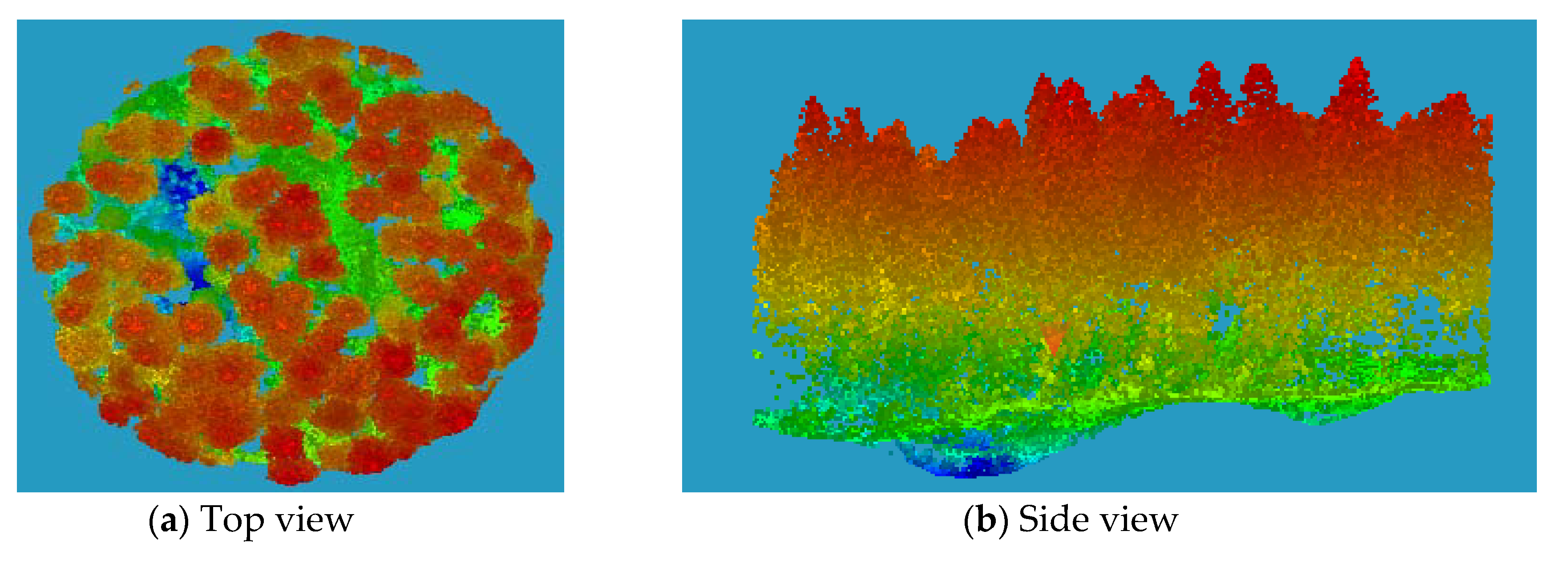
For all study plots, ALS data, DTM, as well as reference data were available in NEWFOR project, and the detailed data used in this article can be downloaded from its website [25]. Since the dataset originates from different institutions, the size and shape of these experimental plots are different. Most of the twelve plots are 40 m in diameter, and some plots (i.e., 3, 10, 11, 12) are 50 m in diameter. For the sake of comparative analysis, this study normalized twelve plots to the same size of 40 m diameter. The 3D view of plot 10 ALS data is shown as an example in Figure 2, where the colour represents the height of point. Red indicates high, and green indicates low.

The region and forest type of experimental plots are presented in Table 1, and more details can be seen in NEWFOR project. Among these plots, 5 plots were multi-layered mixed forests (ML/M), 2 plots were multi-layered coniferous forests (ML/C), 2 plots were single-layered mixed forests (SL/M), and 3 plots are single-layered coniferous forests (SL/C). The field measurements for plots 1, 2, 4, 5, 6, 7, and 8 occurred after the ALS data, while other plots (i.e., 3, 9, 10, 11, 12) had field measurements before the ALS data.

3. Methods

Existing single-tree detection algorithms require selection of the local maxima and thresholds for window dimensions. For example, the watershed method extracts the similar conical geometry of trees. However, this method must select the local maxima as seed points to avoid over-segmentation. The seed point selection depends on the manual setting of the parameters that significantly affects the experimental results.

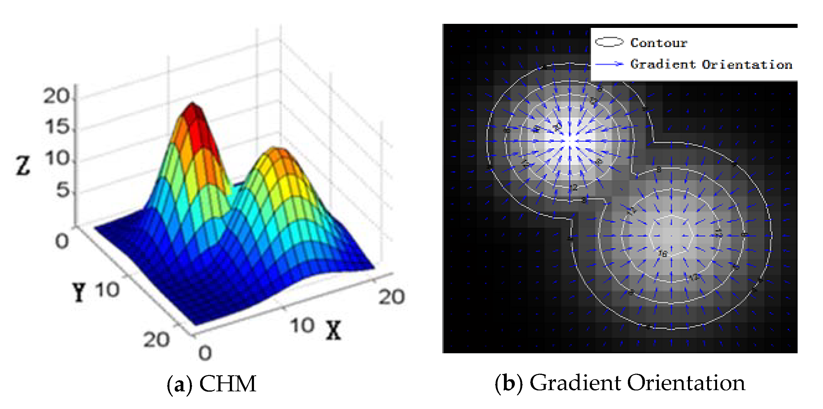
In this study, we proposed a novel and automatic method to detect single trees from ALS data through gradient orientation clustering. Like other single-tree detection algorithms (such as watershed [19,27,28], valley-following [29,30], and active contour model [31,32]), our method considers tree canopies as a mountain-like 3D topographic surface in the rasterized CHM, as shown in Figure 3a. The gradient orientation of each point was calculated from the CHM. The gradient orientation of most points moves towards the local maxima in rasterized CHM, as shown in Figure 3b. If it starts from any point in rasterized CHM and moves along the gradient orientation of each point, it eventually reaches the highest point, which is the local maxima point. All points that reach the same highest point are clustered into the same class. Therefore, the points in the same cones are clustered together.

The process of the proposed method consists of three steps: (1) calculate the DSM based on ALS data by retaining the highest altitude value of the points in each pixel, and then, the CHM is derived by subtracting the DTM from the DSM; (2) obtain the potential single-trees from gradient orientation clustering; and (3) select the final individual trees based on the density feature and determine its coordinates.

3.1. Obtain the CHM from ALS Data

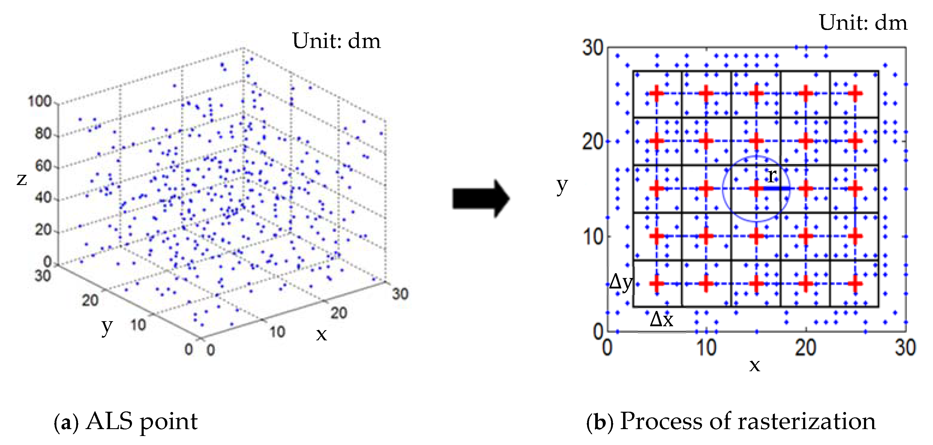
The point cloud in ALS data was irregularly distributed. However, the ALS height values can be summarized into regular grids. Figure 4 is an example of the process of rasterization ALS point cloud data to DSM. In this example, $\Delta x=5\mathrm{dm}$ and $\Delta y=5\mathrm{dm}$ are the length and width of the grid, respectively, and $r=6\mathrm{dm}$ is the search radius of the rasterized pixels. There may be more than one point in the same search range. We set the value of the rasterized pixels to the maximum height values within the search range.

The value will be set to 0 if there is no ALS-information available in a raster cell, which we called black holes. Usually, there are some black holes in the rasterized DSM, which are caused by the abnormal changes of the height values. This unnatural phenomenon may cause potential errors in the treetop detection, but we can solve it through interpolation. Interpolation algorithm is a commonly used algorithm in image processing [33,34]. Usually, there are linear, cubic and nearest-neighbor interpolation methods, and they are integrated into some image processing softwares, such as Matlab (The MathWorks Inc., Natick, MA, USA). What we used is the cubic interpolation method.

As shown in Figure 5, the CHM can be directly subtracted from DSM to DTM. The value of each raster cell in the CHM is the absolute height above ground. The values of some raster cells in the calculated CHM may be less than zero, and those raster cells will be replaced using nearest-neighbour interpolation [35]. Then, a 3 $\times$ 3 Gaussian filtering with σ = 0.5 was used for image smoothing and denoising of the CHM. Section 4.4 will discuss the selection of Gaussian filtering in detail.

3.2. Gradient Orientation Clustering

The x-gradient-component $G_x(x,y)$ of point $(x,y)$ in the CHM can be calculated using the Sobel operator [36]:

$$\begin{array}{c}{G}_x(x,y)=CHM(x-1,y+1)+2CHM(x,y+1)+CHM(x+1,y+1)-\\ CHM(x-1,y-1)-2CHM(x,y-1)-CHM(x+1,y-1)\end{array}$$

(1)

The y-gradient-component $G_y(x,y)$ is

$$\begin{array}{c}{G}_y(x,y)=CHM(x+1,y-1)+2CHM(x+1,y)+CHM(x+1,y+1)-\\ CHM(x-1,y-1)-2CHM(x-1,y)-CHM(x-1,y+1)\end{array}$$

(2)

The gradient orientation $\theta (x,y)$ is

$$\theta (x,y)=\{\begin{array}{lll}\arctan (\frac{G_y(x,y)}{G_x(x,y)})& G_x(x,y)>0& \\ \arctan (\frac{G_y(x,y)}{G_x(x,y)})+\pi & G_y(x,y)\ge 0,G_x(x,y)<0& \\ \arctan (\frac{G_y(x,y)}{G_x(x,y)})-\pi & G_y(x,y)<0,G_x(x,y)<0& ，\theta (x,y)\in [-\pi ,+\pi ]\\ +\frac{\pi }{2}& G_y(x,y)>0,G_x(x,y)=0& \\ -\frac{\pi }{2}& G_y(x,y)<0,G_x(x,y)=0& \\ 0& G_y(x,y)=0,G_x(x,y)=0& \end{array}$$

(3)

The pseudocode of 4-N GOC algorithm (Algorithm 1) is shown as follows.

Algorithm 1. Pseudocode of 4-N GOC.

Input:$CHM\in R^{M\times N}$ Output:$label$ Initialize:$map=\varnothing$, $label\leftarrow 0^{M\times N}$, $index\leftarrow 1$ 1. for $x=1\to M$ 2.  for $y=1\to N$// Traversing every point in the matrix 3.   $(x_c,y_c)\leftarrow (x,y)$// Select a current point from the matrix 4.   if $label(x_c,y_c)==0$ 5.    $map=\varnothing$// Clear the point set 6.     end if 7.     add $(x_c,y_c)$ to $map$ 8.    if $label(x_c,y_c)==0$ 9.    $\begin{array}{l}(x^{\prime },y^{\prime })=\arg min\angle \theta (\alpha ,\beta )\\ (\alpha ,\beta )\in \left\{(x_c+1,y_c),(x_c-1,y_c),(x_c,y_c+1),(x_c,y_c-1)\right\}\end{array}$ 10.     if $CHM(x_c,y_c)>CHM(x^{\prime },y^{\prime })$ 11.     for $(i,j)$ in $map$ 12.      $label(i,j)\leftarrow index$ // Set every point in map 13.      end for 14.      $map=\varnothing$ 15.     $index\leftarrow index+1$ 16.      goto line 2; // Set a new index and start the next cycle 17.    else 18.     $(x_c,y_c)\leftarrow (x^{\prime },y^{\prime })$ 19.     goto line 4 // Set a new current point and do the above steps 20.    end if 21.   else 22.    for $(i,j)$in$map$ 23.     $label(i,j)\leftarrow label(x_c,y_c)$ // Set every point in map 24.    end for 25.   end if 26.   end for 27.  end for

In the 4-N GOC algorithm, $label$ is a label matrix with the size of CHM, which is initialized to 0. These points in $label$ have a same value belong to the same class, (e.g., $label(x,y)=k$ indicates that point $(x,y)$ belongs to class k). $index$ is initialized to 1, and when it increments by 1 indicates that one cluster is completed. $map$ is a point set that stores the points belong to the same class in clustering, and $(i,j)$ represents a point in the $map$. $(x_c,y_c)$ is the point being processed currently. $\angle \theta (\alpha ,\beta )$ is the angle between the gradient orientation $\theta (x_c,y_c)$ and the orientation from $(x_c,y_c)$ to $(\alpha ,\beta )$, where $(\alpha ,\beta )$ represents one neighbour point of $(x_c,y_c)$. $(x^{\prime },y^{\prime })$ is the neighbour point of $(x_c,y_c)$ that has the minimum $\angle \theta (\alpha ,\beta )$.

The gradient orientation clustering (GOC) algorithm is a procedure to find a path from one point to the last point of the cluster. According to the neighbour size, GOC can be divided into 4-N (4-Neighbour) and 8-N (8-Neighbour) GOC algorithms. Compared with Pseudocode of 4-N GOC, Pseudocode of 8-N GOC is only different in line 9 where

$$(\alpha ,\beta )\in \left\{\begin{array}{l}(x_c+1,y_c),(x_c-1,y_c),(x_c,y_c+1),(x_c,y_c-1),\\ (x_c+1,y_c+1),(x_c+1,y_c-1),(x_c-1,y_c+1),(x_c-1,y_c-1)\end{array}\right\}$$

(4)

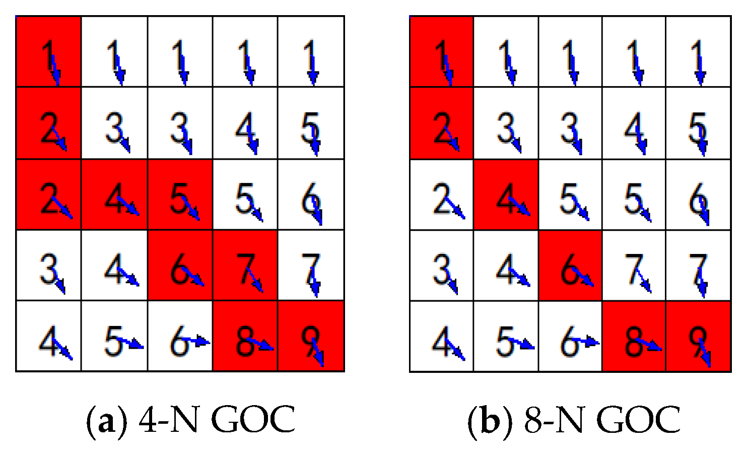
Figure 6 is an example of the process of GOC. During the clustering, both 4-N and 8-N GOC algorithms, the point that is nearest to the current point at the gradient direction is added to the clustering path.

3.3. Single-Tree Selection

In CHM, the gradient orientation of the shrubs and edges of canopies are chaotic. Thus, after the process of gradient orientation clustering, there is some noise and obviously erroneous detection objects in the image, such as rough borders and small plaques. This noise and erroneous detection objects can be eliminated by performing an image morphology opening and closing operation. We had performed some experiments for the morphology opening and closing operation with different structural elements. Finally, the 5 $\times$ 5 square structuring element is selected, as the 3 $\times$ 3 square has a poor smoothing effect, and the 7 $\times$ 7 square may remove some trees correctly detected and distort the image. Although most objects removed are noise and erroneous in the morphology operation, it is inevitable to remove some small trees. For example, if the resolution of CHM is 0.5 m, we will not extract the crown less than 2 m², because the object less than 3 $\times$ 3 cells was removed.

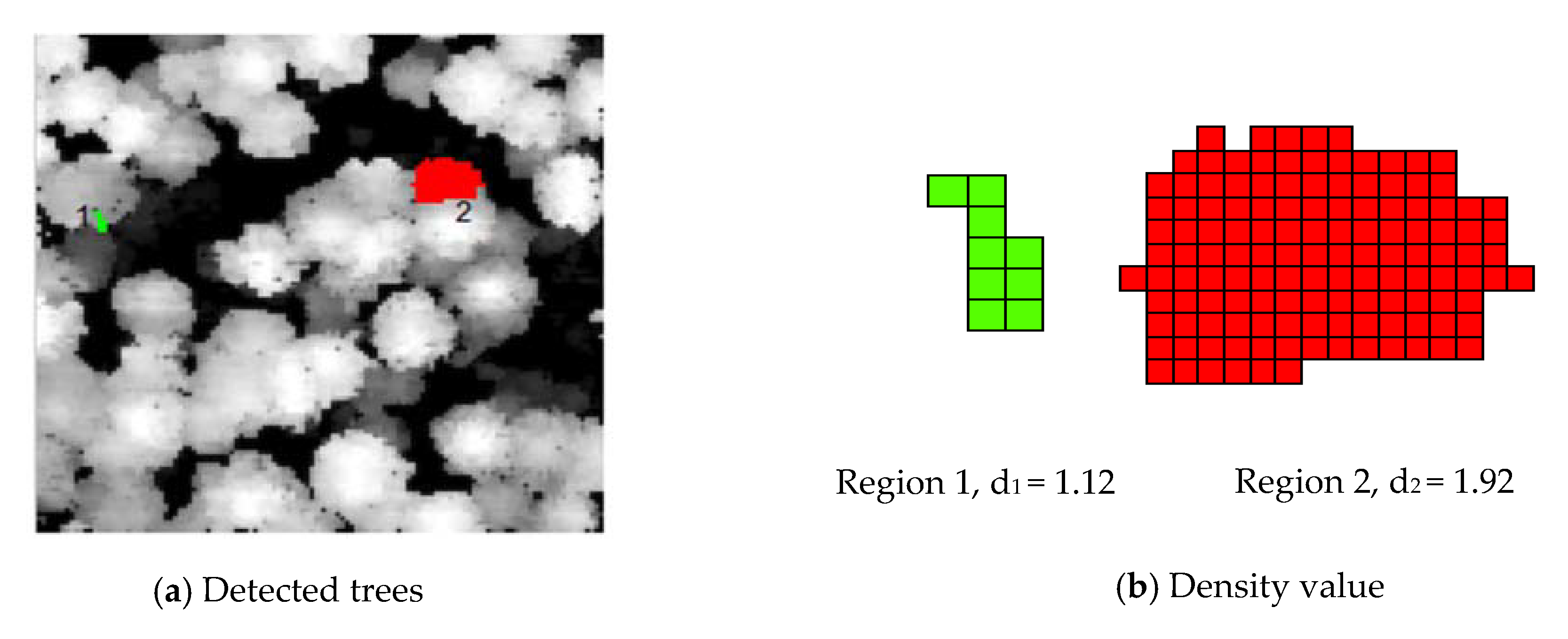
The shape of the tree canopy should approximate a circle. As shown in Figure 7, the object of region 2 is more such as a tree than region 1. The features of the image object that do not satisfy the tree canopy shape must be removed. By defining the density value to describe the compactness of the regions, the noise region (with an abnormal density value) can be removed. The density d is expressed as follows [37]:

$$d=\frac{\sqrt{n}}{1+\sqrt{Var(X)+Var(Y)}}$$

(5)

where n is the number of image pixels for the object; X and Y are the x and y coordinates of all image pixels that constitute the object; and Var is the variance operation. Density d describes the degree of compactness of an object. An image object commonly resembles a square with high density.

We defined the density threshold T_d as follows:

$$T_d=k_1-k_2\times res$$

(6)

where res is the image resolution, $k_1$ and $k_2$ are two constants, and $T_d\in (1,2)$. A higher image resolution corresponds to a larger tree density in the image. Therefore, the appropriate $k_1$ and $k_2$ must be selected to obtain the threshold at different resolutions. $k_1$ is the initial value of a threshold, and $k_1\in [1.2,2]$. Use $k_2$ to adjust the threshold for different resolutions, where $k_2\in [0,1]$. When the density of the image object $d>T_d$, the image object is considered a tree. For example, the density of region 2 in Figure 7a is 1.92, and the density of region 1 in Figure 7a is 1.12. Therefore, the object in region 2 is more likely a tree.

The final step is to determine the centre points of the trees. In this paper, the centre of the minimum circumscribed circle around the image object is considered the centre of a tree. The altitude of the centre point is considered the tree height. The radius of the minimum circumscribed circle is considered the crown radius of a tree. The effect of density features is detailly discussed in Section 4.1.

3.4. Parameters for Accuracy Evaluation

To prove the effectiveness of this method, we analysed the test results of this study with the reference data. The detected tree and reference tree were considered a match if the horizontal difference $\Delta H_{2H}$ and vertical difference $\Delta V_{2V}$ were within a certain range. The matching process is as follows. (1) Candidate tree selection: for a test tree, the reference trees are added to the candidate set if the horizontal difference $\Delta H_{2H}$ and vertical difference $\Delta V_{2V}$ are within a certain threshold range. If the tree is higher than 15 m, we set $\Delta H_{2H}<5 \mathrm{m}$ and $\Delta V_{2V}<2 \mathrm{m}$, else we set $\Delta H_{2H}<4 \mathrm{m}$ and $\Delta V_{2V}<1.5 \mathrm{m}$; (2) Choose the best candidate tree: find the nearest reference tree to the test tree from the candidate set as the best candidate tree; (3) Candidate testing: the matching problem is not a one-way problem. A test tree needs to find the best matching reference tree. The reference tree also needs to find the best matching test tree. These two trees are considered as a successful match only when the candidate tree of the test results and the candidate tree of reference data are two candidate trees for each other.

The evaluation parameters and their calculation methods are defined as follows [26]:

• N_test: Number of extracted trees
• N_ref: Number of reference trees
• N_match: Number of matched trees
• H_mean: Mean horizontal difference of the matching trees
• V_mean: Mean tree height difference of the matching trees
• R_extr (Extraction rate): R_extr = N_test/N_ref
• R_mat (Matching rate): R_mat = N_match/N_ref
• R_com (Commission rate): R_com = (N_test − N_match)/N_test, where commission represents misrecognized of the test result.
• R_om (Omission rate): R_om = (N_ref − N_match)/N_ref, where omission represents leakage recognition of the reference data.

These evaluation parameters were used to measure the matching results for each experimental dataset. The extraction rate should be within a reasonable range. If the extraction rate is too high, (e.g., R_extr = 200%, that indicates at least half of the extracted trees cannot match reference trees, or many extracted trees are incorrect). A higher matching rate indicates a better single-tree detection method. A higher commission rate and omission rate indicate a worse single-tree detection method. Since each above-mentioned indicator can only show one aspect of algorithm performance, we measure the performance of the algorithm more comprehensive and directly by using a matching score. The idea of using a matching score comes from Larsen’s work [38]. In Larsen’s work the matching score is $M_{Laesen}=100\times N_{matching}/(N_{matching}+N_{com}+N_{om})$. In order to make it easier to compare with the previous studies, we modified the matching score as below.

•  M (Matching score): $M=100\times \frac{R_{mat}}{R_{mat}+R_{com}+R_{om}}$

Although the expressions of these two formulas are different, a high matching score under our criteria can also indicate that the algorithm performance is better. In addition, root mean square (RMS) was used to evaluate the accuracy of model predictions. The evaluation parameters of the RMS were defined as follows [26]:

• RMS_H: Root mean square of H_mean.
• RMS_V: Root mean square of V_mean.
• RMS_R_extr: Root mean square of R_extr.
• RMS_R_mat: Root mean square of R_mat.
• RMS_R_com: Root mean square of R_com.
• RMS_R_om: Root mean square of R_om.
• RMS_M: Root mean square of matching score.

The RMS of X is defined as Formula (7), where X can be H_mean, V_mean, R_extr, R_mat, R_com, R_om and M, i represents the i-th plot.

$$RMS\_X=\sqrt{\frac{1}{n}{\displaystyle \sum _1^n{X}_i^2}}$$

(7)

4. Experiment & Discussion

This section aims to verify the effectiveness of our algorithm by conducting some related experiments. Firstly, it shows the selection of appropriate parameters, such as 4-N or 8-N GOC, different resolutions, different Gaussian filters, the values of k₁, k₂ and T_d. Next, it shows the results of 4-N GOC and 8-N GOC for each plot, and evaluates the detection results by using the evaluation criteria, such as extraction rate, matching rate, commission rate, omission rate, mean horizontal distance and mean height distance. Then, to show the advantages of our method, it presents the experiment results of RMS_R_extr, RMS_R_mat, RMS_R_com, RMS_R_om, RMS_H, and RMS_V for 12 plots to compare the detection results of our method with other existing methods. Finally, it presents the applicability of our algorithm for different forest types.

4.1. Analysis of Model Parameters

This section mainly presents the selection of experimental parameters. It first shows the effects of using different Gaussian filters. Then, it shows the effects of density threshold. Finally, it presents the effects of 4-N and 8-N and the effects of different resolutions of rasterized CHM.

We have tried several filter-specifications such as 3 × 3, 5 × 5 and 7 × 7 filtering to smoothen the CHM. With the same window size, there is almost no difference in the performances for different $\sigma$ values, so in our experiment we chose $\sigma =0.5$.

Table 2. Matching Scores of all Plots and their RMS_M for different Gaussian filters.

	Plot_ID	1	2	3	4	5	6	7	8	9	10	11	12	RMS_M
Size
no filtering		42	44	43	37	25	56	49	36	31	39	54	34	41
3 × 3		43	46	44	34	29	56	52	31	36	45	48	49	43
5 × 5		43	46	43	34	29	56	51	31	37	45	48	50	43
7 × 7		44	46	42	48	35	53	45	31	38	45	41	45	42

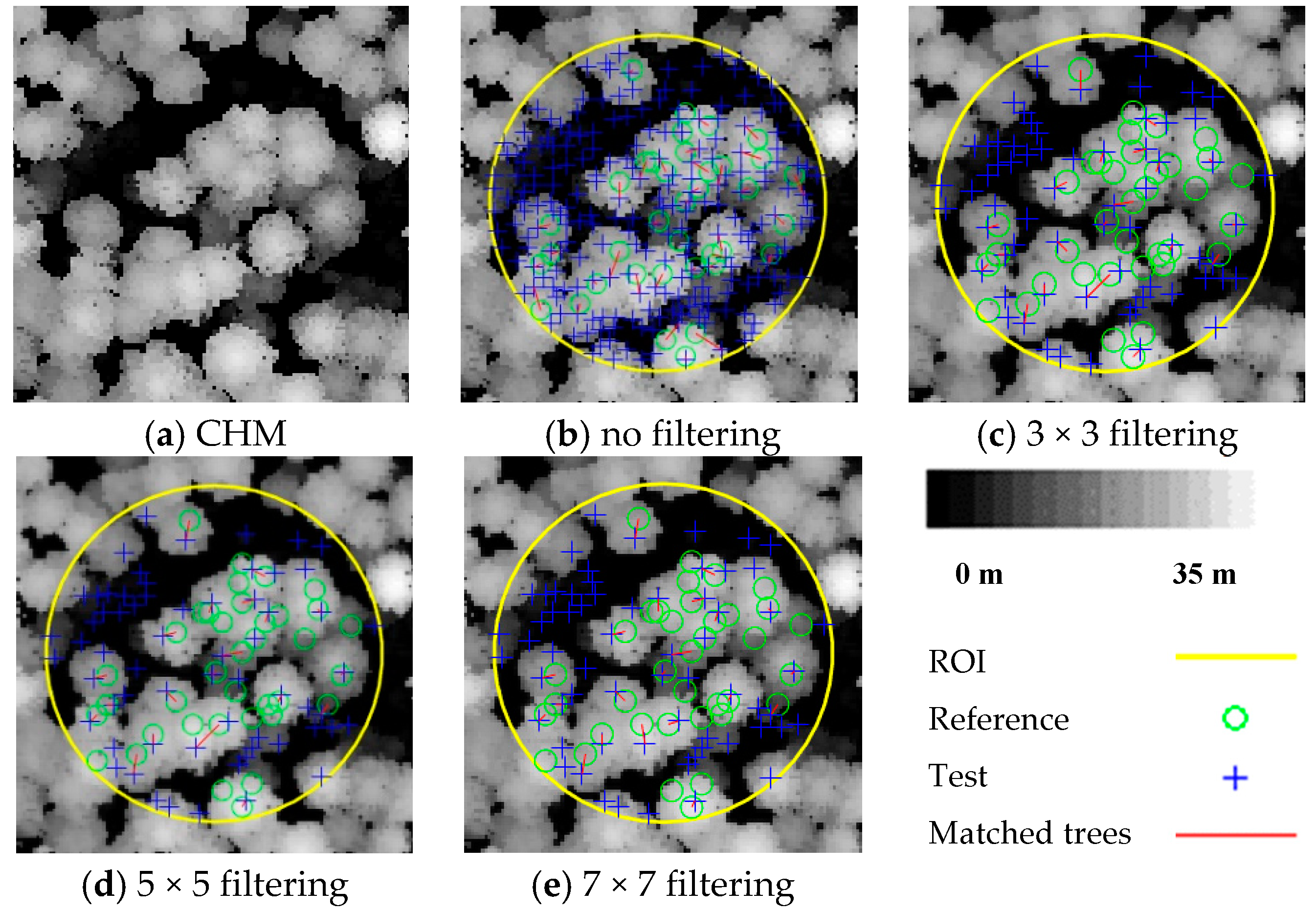
RMS_M: root mean square matching score.

shows matching scores of all 12 plots and there RMS_M of no filter, 3 $\times$ 3, 5 $\times$ 5 and 7 $\times$ 7 Gaussian filters. Moreover, Figure 8 shows 0.5 m CHM and the matching results of no filter, 3 $\times$ 3, 5 $\times$ 5 and 7 $\times$ 7 Gaussian filters in plot 10 using 4-N GOC method as an example. As we can see, the matching score M of no filter, 3 $\times$ 3, 5 $\times$ 5 and 7 $\times$ 7 Gaussian filters in plot 10 are 39, 45 45, 45. For plot 10, the detection result for the CHM using filter was better than the CHM without filter, and the single tree detection using different gaussian filters almost had the same results. Moreover, RMS_M of all these twelve plots showed that the detection result for the CHM using filter will have better performance than the CHM without filter. For these filters, the 3 $\times$ 3 and 5 $\times$ 5 filter had a better performance.

For the impact of density threshold T, we also took plot 10 as an example.

Table 3. Matching results of plot 10 with density threshold T_d of 0, 1.2, 1.4, and 1.6 respectively.

	Plot_ID	Ntest	Nref	Nmatch	Rextr	Rmat	Rcom	Rom	Hmean	Vmean	M
Td
0		91	37	29	246%	78%	68%	22%	1.7 m	1.2 m	46
1.2		64	37	28	173%	76%	76%	24%	1.8 m	1.2 m	49
		55	37	27	149%	73%	51%	27%	1.9 m	1.3 m	48
1.4		35	37	24	95%	65%	31%	35%	1.8 m	1.2 m	49

shows the matching results of plot 10 with T_d of 0, 1.2, 1.4, and 1.6 respectively. The extracted number decreases quickly when the threshold increases, and the matched number decreases rarely. Simply said, the density threshold T_d can help reduce the commission rate. Moreover, R_om does not increase with the same rate as R_com decreases. Therefore, the matching score M by setting the density threshold T_d will have better performance. When the threshold is within a certain range (1.2 to 1.6), the impact on the result is not significant.

In addition, we used two detection methods to present the experimental results: 4-N and 8-N gradient orientation clustering. The resolution of the CHM significantly affects the experimental results. If the density of the ALS data is not sufficient to support a high-resolution CHM, the CHM will have many null points. Although they can be filled using the interpolation method, this problem inevitably increases the noise in the CHM. If the CHM resolution is too low, the information in the CHM to compute the gradient orientation is inadequate and inaccurate. Then, the detection rate decreases; in particular, some small trees cannot be detected. To compare the experimental results, we generated three different resolution (0.3 m, 0.5 m, 0.7 m) CHM in this paper.

Table 4. Effects of different parameters on the matching results in single-tree detection.

Method	Resolution	k1, k2	Td	RMS_M
4-N	0.3 m	1.7, 0.65	1.505	36
		1.55, 0.5	1.4	37
		1.4, 0.35	1.295	37
	0.5 m	1.7, 0.65	1.375	41
		1.55, 0.5	1.3	43
		1.4, 0.35	1.225	43
	0.7 m	1.7, 0.65	1.245	38
		1.55, 0.5	1.2	37
		1.4, 0.35	1.155	37
8-N	0.3 m	1.7, 0.65	1.505	40
		1.55, 0.5	1.4	40
		1.4, 0.35	1.295	40
	0.5 m	1.7, 0.65	1.375	36
		1.55, 0.5	1.3	36
		1.4, 0.35	1.225	36
	0.7 m	1.7, 0.65	1.245	33
		1.55, 0.5	1.2	33
		1.4, 0.35	1.155	32

shows different parameters and the experimental results for all datasets. The three groups of k₁ and k₂ have notably similar experiment results, which implies that the parameters have a minimal effect on the single-tree matching result.

The best matching result is obtained when k₁ is 1.55 and k₂ is 0.5. Therefore, in our experiments, the values of k₁ and k₂ can be set as 1.55 and 0.5, respectively. We do not need manually adjust the values of these parameters according to the spatial resolutions of remote-sensing images, which enable the automation of single-tree detection.

Table 5. Matching results of 4-N gradient orientation clustering (GOC) and 8-N GOC at different resolutions. 4-N GOC achieves more satisfactory results at 0.5 m resolution.

Resolution	Method	RMS_Rextr (%)	RMS_Rmat (%)	RMS_Rcom (%)	RMS_Rom (%)	RMS_H (m)	RMS_V (m)	RMS_M
0.3 m	4-N	149	57	49	49	2.0	1.1	37
	8-N	249	68	62	36	2.0	1.0	41
0.5 m	4-N	124	63	42	42	1.9	1.0	43
	8-N	108	53	43	50	1.9	1.0	36
0.7 m	4-N	65	48	23	54	1.9	0.8	38
	8-N	59	42	28	60	1.8	0.9	32

shows the 4-N GOC and 8-N GOC matching results for CHM at 0.3 m, 0.5 m, and 0.7 m resolutions over the entire dataset. The 4-N GOC single-tree detection method achieved relatively satisfactory results at 0.5 m resolution. If the resolution of CHM is too high or too low, the results will not be reasonable. If the CHM resolution is too high, the point density is sparse, which results in more noise in the CHM. If the CHM resolution is too low, too much gradient information is lost in the CHM.

As to the reason that 4-N GOC performs better than 8-N GOC in our algorithm, the remote sensing image is not clear enough, so the gradient information is partly incorrect. In 8-N GOC, one raster cells will have eight directions to point to, and there are less raster cells point to a same one compared with 4-N GOC. Therefore, the clustering of 8-N is easy to converge prematurely, that results in an error clustering, which can be verified from the commission rate. As we can see in Table 5, the commission rate of 8-N GOC is higher than that of 4-N GOC no matter what the extraction rate is. Therefore, we finally adopted 4-N GOC in our comparative experiment.

4.2. Results for Each Plot of the Dataset

This section gives the results of each plot and the evaluation results of relevant six parameters (extraction rate, matching rate, commission rate, omission rate, mean horizontal distance and mean height distance) of 4-N GOC and 8-N GOC for each plot with the 0.3 m, 0.5 m and 0.7 m CHM.

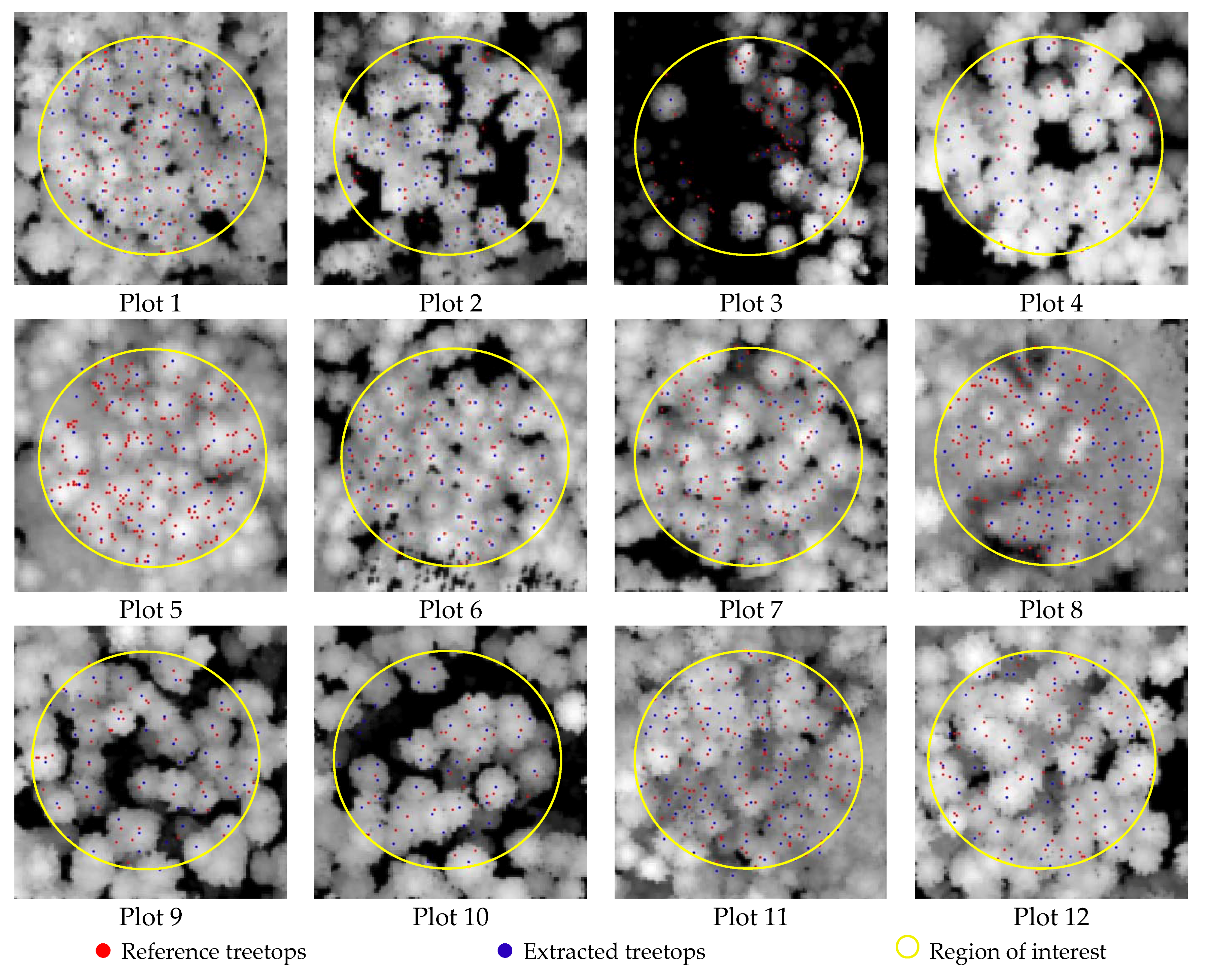
This study conducted the proposed single-tree detection algorithm in twelve plots of approximately 20 metres in diameter, which belonged to multi-layered mixed forests (ML/M), multi-layered coniferous forests (ML/C), single-layered mixed forests (SL/M), and single-layered coniferous forests (SL/C), as shown in Table 1. Figure 9 illustrates the results of the extracted individual trees by the 4-N GOC method with 0.5 m CHM.

In this study, there were 1286 reference trees, and a total of 1189 trees were extracted using the proposed algorithm in these twelve plots. The forest type of plots 1 and 3 were ML/C, and plots 2, 4, and 6 were SL/C. They were composed of coniferous trees, and the gradient of a coniferous tree usually points to only one treetop, so these plots had good extracted rates. The main problem of these plots was the omission rate. The forest type of plots 5, 7, 8, 11, and 12 were ML/M, and that of plots 9 and 10 was SL/M. They are mixed forests of conifer and broadleaf trees. As the gradient of a broadleaf tree may point to multiple treetops, the commission rate of these plots was slightly high. Overall, the proposed algorithm extracted most individual treetops in four types of forests. The matching score was M = 39 for ML/C plots, M = 51 for SL/C plots and M = 39 for ML/M plots, and M = 47 for SL/M plots. However, there were some omitted and misrecognized trees in each plot. We will discuss the matching results for different forest types in Section 4.4.

In Figure 10a, the extraction rate is higher when the resolution of the CHM resolution is higher, but the extraction rate being too high is not necessarily a good thing. It will also result in a high commission rate. The extraction rate should be in a suitable range (e.g., 50% to 150%). Then, we counted the plot number of 4-N and 8-N GOC’s extraction rate in a suitable range in total of 0.3 m, 0.5 m and 0.7 m are 11, 17, and 19, respectively.

A higher resolution corresponds to a higher matching rate because the extraction rate is high at high resolution, where more trees are accurately extracted at the same time, and the matching rate increases. At low resolution, the extraction rate is low and the number of accurately extracted trees decreases. Therefore, the matching rate in the single-tree detection is low. A higher matching rate is better, but we think that a result with greater than 60% the matching rate is a relatively good result. As in Figure 10b, 4-N GOC and 8-N GOC in 0.5 m CHM achieved the most plots with an excellent result. There were 10 plots of 4-N GOC with excellent results at 0.5 m resolution. These 10 plots include all single-layered forests (plots 2, 4, 6, 9 and 10), which indicates that the method achieves good results for single-layered forest types.

The commission is the misrecognized trees in the detection results; thus, the commission rate increase with the extraction rate increase. As seen in Figure 10c, the commission rates in 0.3 m CHM are higher than in 0.5 m and 0.7 m CHM. Because the density of ALS points in a pixel of the rasterized CHM of 0.3 m resolution is low, the 0.3 m CHM contains more noise; therefore, there are more misrecognized trees in the detection results. The omission is leakage in the reference trees, so the omission rate increases with the extraction rate decrease. As seen in Figure 10d, the omission rates in 0.7 m CHM are higher than that in 0.3 m and 0.5 m CHM. Too much gradient information is lost when generating CHM with 0.7 m resolution with ALS point cloud data, and the trees density feature in low resolution CHM is difficult to recognize. Figure 10e,f show the mean horizontal and vertical distance between the matched trees and reference trees. The mean horizontal distance of 0.3 m, 0.5 m, 0.7 m CHM is 2.0 m, 1.9 m and 1.9 m respectively. The mean vertical distance of 0.3 m, 0.5 m, 0.7 m CHM is 1.1 m, 1.0 m and 0.9 m, respectively. The mean horizontal and vertical distance difference between CHM of the three resolutions is small. Through the above histogram of six evaluation parameters, we find that the proposed 4-N GOC and 8-N GOC achieve best result in CHM of 0.5 m resolution.

4.3. Comparison with Previous Studies

To verify the effectiveness of the proposed GOC method, we conducted a comparative experiment with eight previous single-tree detection methods. The experimental results (i.e., RMS_R_extr, RMS_R_mat, RMS_R_com, RMS_R_om, RMS_H, RMS_V) of these eight methods are provided in the study of Eysn et al. [26]. Although these indicators are very specific, it is difficult to directly know the effect of the algorithm. Therefore, we calculated the root mean square of matching scores (RMS_M), which can directly compare the performance of these algorithms. In order to make it easier to compare with the other algorithms compared by Eysn et al., we modified Larsen’s formula of matching score. Although the expressions of these two formulas are different, the ideas of computing matching score are basically consistent. Moreover, our method can produce similar results when N_ref = N_test.

Table 6. Matching results of single-tree detection methods. Our single-tree detection method with 4-N GOC achieves a maximum RMS_M over the dataset.

ID	Method	RMS_Rextr	RMS_Rmat	RMS_Rcom	RMS_Rom	RMS_H	RMS_V	RMS_M
1	LM + filtering	51%	45%	9%	59%	1.6 m	0.9 m	40
2	LM + region growing	57%	43%	20%	61%	1.8 m	1.2 m	35
3	LM + multi CHM	101%	46%	61%	57%	1.7 m	0.7 m	28
4	LM + Watershed	86%	49%	49%	55%	1.6 m	1.1 m	32
5	Segment + Clustering	139%	53%	95%	51%	1.7 m	1.0 m	27
6	LM 3 × 3	154%	54%	113%	51%	1.6 m	0.9 m	25
7	LM 5 × 5	52%	41%	16%	63%	1.8 m	1.1 m	34
8	Polyn. Fitting + Watershed	54%	44%	13%	59%	1.8 m	1.1 m	38
9	GOC	124%	63%	42%	42%	1.9 m	1.0 m	43

shows the matching results of various single-tree detection methods. The ninth method is our method with 4-N GOC at 0.5 m resolution. The single-tree detection method with 4-N GOC can achieve a 63% matching rate at 124% extraction rate, which is much higher than the other detection methods. The commission rate in our method is 42%, which is lower than those of methods 3, 4, 5, and 6. The omission rate in our method is 42%, which is lower than any other method. RMS_H is 1.9 m, which is slightly higher than those of other methods; RMS_V is 1.0 m, which can reach the average level of all other methods. For the RMS_M, our single-tree detection method of 4-N GOC achieves a maximum RMS_M over the entire dataset. Therefore, the 4-N GOC is an excellent single-tree detection method to detect single trees from the ALS data.

For further experiments, we also have implemented the related algorithms. For example, we compared the matching results using our method with LM + filtering [39]. Figure 11 shows the matching results for 4-N GOC and the LM + filtering method.

Figure 11a shows the matching results of 4-N GOC with 0.5 m resolution in plot 10 using 4-N GOC method. The extraction rate is 170%, the matching rate is 76%, the commission rate is 56%, the omission rate is 24%, and the matching score is 49. Figure 11b,c use the LM + filtering. In Figure 11b, the window size is 5, the extraction rate is 91%, the matching rate is 59%, the commission rate is 35%, the omission rate is 41%, and the matching score is 44. In Figure 11c, the window size is 3, the extraction rate is 329%, the matching rate is 81%, the commission rate is 75%, the omission rate is 19%, and the matching score is 46. The results show that the 4-N GOC method can provide superior results, whereas the LM + filtering method is strongly affected by the window size.

4.4. Analysis of Matching Results for Different Forest Types

The existing single-tree detection methods based on rasterized CHM are commonly used to detect trees in a single-layered forest or dominant trees in a multi-layered forest. It is difficult to effectively detect suppressed trees in a multi-layered forest. Though GOC cannot detect suppressed trees in a multi-layered forest either, it can appropriately capture the dominant trees at least.

To explore the effect of the GOC algorithm on different types of forests, we applied our method to detect single trees in both single-layered forests and multi-layered forests.

Table 7. Matching results for different forest types.

Forest Type	SL/M	SL/C	ML/M	ML/C
RMS_Rext	163%	139%	116%	74%
RMS_Rmat	73%	73%	57%	52%
RMS_Rcom	54%	44%	41%	30%
RMS_Rom	27%	27%	48%	50%
RMS_H	1.8 m	1.7 m	2.0 m	1.7 m
RMS_V	1.1 m	1.0 m	0.9 m	1.1 m
RMS_M	47	51	39	39

SL/M: single-layered mixed forests; SL/C: single-layered coniferous forests; ML/M: multi-layered mixed forests; ML/C: multi-layered coniferous forests.

shows the matching results for different types of forests using our 4-N GOC method at 0.5 m resolution. According to the matching results, there are larger values of RMS_R_extr, RMS_R_mat and RMS_R_com in single-layered mixed forests and single-layered coniferous forests. The values of RMS_M are 47 and 51 for the single-layered mixed forests and single-layered coniferous forests, respectively. Therefore, our single-tree detection method is more suitable for non-overlapping trees in a single-layered forest.

Because CHM only contains the top layer information of the tree canopy, that leads to better performance of the algorithm in single-layer forests than multi-layer forests. The matching results of multi-layered mixed forests and multi-layered coniferous forests have smaller values of RMS_R_extr, RMS_R_mat and RMS_R_com than those of the single-layered forest. The values of RMS_M for the multi-layered mixed forest and multi-layered coniferous forest is 39. Although the matching results of the multi-layered forest are not as satisfactory as those of single-layered forests, they are still better than most the other existing methods in Table 6. Therefore, GOC method can also be used to automatically and effectively identify dominant trees in multi-layered forests.

5. Conclusions

This paper proposed an automatic method for single-tree detection in airborne laser scanning data through gradient orientation clustering. The proposed method combines the height value of CHM and gradient orientation information to cluster points belonging to the same crown as a conical shape in a canopy to detect single-trees. In the experiments, we used the proposed method with two different neighbour sizes (4-N and 8-N), and we presented the experimental results in six different aspects, the extraction rate, matching rate, commission rate, omission rate, mean horizontal distance and mean height distance. In our method, the CHM resolution significantly affects the experimental results. If the ALS points density is not sufficient to support a high-resolution CHM, the CHM may have some pits. Although they can be filled by using the linear interpolation method, this problem inevitably distorts the CHM. If the CHM resolution is too low, the gradient orientation information of the CHM is inadequate and inaccurate. This result in the extraction rate and matching rate obviously decreasing and many small trees cannot be detected. Experiment shows that the overall matching scores of the proposed GOC method in four types of forests are higher than those of the other eight methods, and the root mean square matching score of GOC method (RMS_M is 43) at least 7% higher than the other eight methods. Although the proposed method can detect dominant single trees in multi-layered forests, this method has more satisfactory results in single-layered forests.

As to the types of forest communities, such as the broad-leaved forest, coniferous forest, and mixed coniferous broad-leaved forest, as long as the tree crown has a conical shape, our method is applicable. However, the single-tree detection method still has room for improvement, particularly for the detection of multi-layer forest, as the information for different layers of the multi-layered forest is insufficient in the CHM. Because of GOC method needs to calculate the gradient orientation of the trees and small trees’ gradient orientation have deviation, it is not suitable for small trees’ detection. For example, GOC cannot correctly detect the crown whose projection area is below 2 m². In the future, our method will be combined with a point cloud-based method to detect small trees and find a way to detect the suppressed trees in multi-layered forests.

References

1. Kumar, J.; Talwar, P.; Krishna, A. Forest Canopy Density and ASTER DEM based Study for Dense Forest Investigation using Remote Sensing and GIS Techniques around East Singhbhum in Jharkhand, India. Int. J. Adv. Remote Sens. GIS 2015, 4, 1026–1032. [Google Scholar] [CrossRef]
2. Nagendra, H.; Lucas, R.; Honrado, J.P.; Jongman, R.H.; Tarantino, C.; Adamo, M.; Mairota, P. Remote sensing for conservation monitoring: Assessing protected areas, habitat extent, habitat condition, species diversity, and threats. Ecol. Indic. 2013, 33, 45–59. [Google Scholar] [CrossRef]
3. Garestier, F.; Dubois-Fernandez, P.C.; Champion, I. Forest height inversion using high-resolution P-band Pol-InSAR data. IEEE Trans. Geosci. Remote Sens. 2008, 46, 3544–3559. [Google Scholar] [CrossRef]
4. Deo, R.K.; Russell, M.B.; Domke, G.M.; Andersen, H.E.; Cohen, W.B.; Woodall, C.W. Evaluating Site-Specific and Generic Spatial Models of Aboveground Forest Biomass Based on Landsat Time-Series and LiDAR Strip Samples in the Eastern USA. Remote Sens. 2017, 9, 598. [Google Scholar] [CrossRef]
5. Yu, B.; Liu, H.; Wu, J. A method for urban vegetation classification using airborne LiDAR data and high resolution remote sensing images. J. Image Graph. 2010, 15, 782–789. [Google Scholar]
6. Zhen, Z.; Quackenbush, L.J.; Zhang, L. Trends in automatic individual tree crown detection and delineation—Evolution of LiDAR data. Remote Sens. 2016, 8, 333. [Google Scholar] [CrossRef]
7. Hyyppä, J.; Schardt, M.; Haggrén, H.; Koch, B.; Lohr, U.; Scherrer, H. HIGH-SCAN: The first European-wide attempt to derive single-tree information from laserscanner data. Photogramm. J. Finl. 2001, 17, 58–68. [Google Scholar]
8. Popescu, S.C.; Wynne, R.H. Seeing the trees in the forest. Photogramm. Eng. Remote Sens. 2004, 70, 589–604. [Google Scholar] [CrossRef]
9. Koch, B.; Heyder, U.; Weinacker, H. Detection of individual tree crowns in airborne lidar data. Photogramm. Eng. Remote Sens. 2006, 72, 357–363. [Google Scholar] [CrossRef]
10. Hyyppä, J.; Holopainen, M.; Olsson, H. Laser scanning in forests. Mol. Divers. Preserv. Int. 2012, 4, 2919–2922. [Google Scholar] [CrossRef]
11. Corona, P.; Cartisano, R.; Salvati, R.; Chirici, G.; Floris, A.; Di Martino, P. Airborne Laser Scanning to support forest resource management under alpine, temperate and Mediterranean environments in Italy. Eur. J. Remote Sens. 2012, 45, 27–37. [Google Scholar] [CrossRef] [Green Version]
12. Nijland, W.; Coops, N.C.; Nielsen, S.; Stenhouse, G. Integrating optical satellite data and airborne laser scanning in habitat classification for wildlife management. Int. J. Appl. Earth Obs. Geoinf. 2015, 38, 242–250. [Google Scholar] [CrossRef]
13. Maltamo, M.; Næsset, E.; Vauhkonen, J. Forestry Applications of Airborne Laser Scanning: Concepts and Case Studies; Springer: Berlin, Germany, 2014. [Google Scholar]
14. Hyyppa, J.; Kelle, O.; Lehikoinen, M.; Inkinen, M. A segmentation-based method to retrieve stem volume estimates from 3-D tree height models produced by laser scanners. IEEE Trans. Geosci. Remote Sens. 2001, 39, 969–975. [Google Scholar] [CrossRef]
15. Persson, A. Detecting and measuring individual trees using an airborne laser scanner. Photogramm. Eng. Remote Sens. 2002, 68, 925–932. [Google Scholar]
16. Popescu, S.C.; Wynne, R.H.; Nelson, R.F. Estimating plot-level tree heights with lidar: Local filtering with a canopy-height based variable window size. Comput. Electron. Agric. 2002, 37, 71–95. [Google Scholar] [CrossRef]
17. Chen, Q.; Baldocchi, D.; Gong, P.; Kelly, M. Isolating individual trees in a savanna woodland using small footprint lidar data. Photogramm. Eng. Remote Sens. 2006, 72, 923–932. [Google Scholar] [CrossRef]
18. Ke, Y.; Quackenbush, L.J. A review of methods for automatic individual tree-crown detection and delineation from passive remote sensing. Int. J. Remote Sens. 2011, 32, 4725–4747. [Google Scholar] [CrossRef]
19. Wang, L.; Gong, P.; Biging, G.S. Individual tree-crown delineation and treetop detection in high-spatial-resolution aerial imagery. Photogramm. Eng. Remote Sens. 2004, 70, 351–357. [Google Scholar] [CrossRef]
20. Dalponte, M.; Frizzera, L.; Gianelle, D. Estimation of forest attributes at single tree level using hyperspectral and ALS data. Remote Sens. Environ. 2014, 79, 105–115. [Google Scholar]
21. Mohan, M.; Silva, C.A.; Klauberg, C.; Jat, P.; Catts, G.; Cardil, A.; Hudak, A.T.; Dia, M. Individual Tree Detection from Unmanned Aerial Vehicle (UAV) Derived Canopy Height Model in an Open Canopy Mixed Conifer Forest. Forests 2017, 8, 340. [Google Scholar] [CrossRef]
22. Zhao, Y.; Hao, Y.; Zhen, Z.; Quan, Y. A Region-Based Hierarchical Cross-Section Analysis for Individual Tree Crown Delineation Using ALS Data. Remote Sens. 2017, 9, 1084. [Google Scholar] [CrossRef]
23. Kaartinen, H.; Hyyppä, J.; Yu, X.; Vastaranta, M.; Hyyppä, H.; Kukko, A.; Holopainen, M.; Heipke, C.; Hirschmugl, M.; Morsdorf, F.; et al. An International Comparison of Individual Tree Detection and Extraction Using Airborne Laser Scanning. Remote Sens. 2012, 4, 950–974. [Google Scholar] [CrossRef] [Green Version]
24. Vauhkonen, J.; Ene, L.; Gupta, S. Comparative testing of single-tree detection algorithms under different types of forest. Forestry 2011, 85, 27–40. [Google Scholar] [CrossRef]
25. NEWFOR. The NEWFOR Single Tree Detection Benchmark Dataset. Available online: http://www.newfor.net/download-newfor-single-tree-detection-benchmark-dataset/ (accessed on 1 Feburary 2015).
26. Eysn, L.; Hollaus, M.; Lindberg, E.; Berger, F.; Monnet, J.-M.; Dalponte, M. A benchmark of lidar-based single tree detection methods using heterogeneous forest data from the alpine space. Forests 2015, 6, 1721–1747. [Google Scholar] [CrossRef] [Green Version]
27. Wannasiri, W.; Nagai, M.; Honda, K.; Santitamnont, P.; Miphokasap, P. Extraction of Mangrove Biophysical Parameters Using Airborne LiDAR. Remote Sens. 2013, 5, 1787–1808. [Google Scholar] [CrossRef]
28. Lamar, W.R.; Mcgraw, J.B.; Warner, T.A. Multitemporal censusing of a population of eastern hemlock (Tsuga canadensis L.) from remotely sensed imagery using an automated segmentation and reconciliation procedure. Remote Sens. Environ. 2005, 94, 133–143. [Google Scholar] [CrossRef]
29. Gougeon, F.A. A Crown-Following Approach to the Automatic Delineation of Individual Tree Crowns in High Spatial Resolution Aerial Images. Can. J. For. Res. 1995, 21, 274–284. [Google Scholar] [CrossRef]
30. Gougeon, F.A.; Leckie, D.G. The individual tree crown approach applied to Ikonos images of a coniferous plantation area. Photogramm. Eng. Remote Sens. 2006, 72, 1287–1297. [Google Scholar] [CrossRef]
31. Lin, C.; Thomson, G.; Lo, C.S.; Yang, M.S. A multi-level morphological active contour algorithm for delineating tree crowns in mountainous forest. Photogramm. Eng. Remote Sens. 2011, 77, 241–249. [Google Scholar] [CrossRef]
32. Ardila, J.P.; Bijker, W.; Tolpekin, V.A. Multitemporal change detection of urban trees using localized region-based active contours in VHR images. Remote Sens. Environ. 2012, 124, 413–426. [Google Scholar] [CrossRef]
33. Isenburg, M. LAStools—Efficient Tools for LiDAR Processing. Available online: http://www.cs.unc.edu/~isenburg/lastools/ (accessed on 9 October 2012).
34. Oliver, M.A.; Webster, R. Kriging: A method of interpolation for geographical information systems. Int. J. Geogr. Inf. Syst. 1990, 4, 313–332. [Google Scholar] [CrossRef]
35. Collignon, A.; Maes, F.; Delaere, D. Automated multi-modality image registration based on information theory. Inf. Process. Med. Imaging 1995, 3, 263–274. [Google Scholar]
36. Gonzalez, R.; Woods, R. Digital Image Processing; Addison Wesley: Boston, MA, USA, 1992; pp. 414–428. [Google Scholar]
37. eCognition. eCognition® Developer (8.64.0) Reference Book; Trimble Germany GmbH: Munich, Germany, 2010. [Google Scholar]
38. Larsen, M.; Eriksson, M.; Descombes, X. Comparison of six individual tree crown detection algorithms evaluated under varying forest conditions. Int. J. Remote Sens. 2011, 32, 5827–5852. [Google Scholar] [CrossRef]
39. Monnet, J.M.; Mermin, E.; Chanussot, J. Tree top detection using local maxima filtering: A parameter sensitivity analysis. In Proceedings of the 10th International Conference on LiDAR Applications for Assessing Forest Ecosystems (Silvilaser 2010), Freiburg, Germany, 14–17 September 2010. [Google Scholar]
Figure 1. Study areas distribution. Red triangles represent different study areas that this paper used, and yellow triangles represent the remaining areas of NEWFOR (NEW technologies for a better mountain FORest timber mobilization) project.
Forests 09 00291 g001
Figure 2. 3D view of ALS data.
Forests 09 00291 g002
Figure 3. Three-dimensional display of canopy height model (CHM) (a) and gradient orientation (b).
Forests 09 00291 g003
Figure 4. The process of rasterizing ALS point cloud data to the digital surface model (DSM). The blue point represent the ALS point. The black rectangles represent the rasterized pixels and the red cross represents the value of a rasterized pixel.
Forests 09 00291 g004
Figure 5. Computing canopy height within each pixel based on the difference between the surface model and the terrain model. DSM = digital surface model; DTM = digital terrain model; CHM = canopy height model.
Forests 09 00291 g005
Figure 6. Example of gradient orientation clustering (GOC). The blue arrow represents the gradient orientation of a point and the red squares represent the clustering path.
Forests 09 00291 g006
Figure 7. An example of single-tree selection based on density feature. The green pixels and the red pixels represent region 1 and region 2, respectively.
Forests 09 00291 g007
Figure 8. Matching results of no filter, 3 × 3, 5 × 5, and 7 × 7 Gaussian filters.
Forests 09 00291 g008
Figure 9. Results for each plot of the dataset.
Forests 09 00291 g009
Figure 10. The evaluation parameters for each plot of the study plots (the raster resolutions are 0.3, 0.5, and 0.7 m respectively, and the numbers indicate the plot IDs).
Forests 09 00291 g010aForests 09 00291 g010b
Figure 11. Matching results of 4-N GOC and LM + filtering methods.
Forests 09 00291 g011