1. Introduction
Ecological modeling has proven to be an effective approach toward understanding key factors that influence or control the long-term behavior of a system of interest. Among these, the individual-based gap models (IBGMs) have a long history of successful forest simulation across temperate and northern forests (See: [
1] for recent review). Establishment, diameter growth, and mortality of trees are usually simulated on an annual time-step, within a plot of a defined size. As a defining characteristic of IBGMs, the life history of each individual is simulated as a unique entity with respect to these processes [
2,
3,
4]. For each individual, simple interaction rules (e.g., shading, competition for limiting resources, etc.) in conjunction with rules for birth, death, and growth are the basis for individual response functions, which are driven by the formation of canopy gaps that occur when a mature tree falls [
1,
2,
3,
5]. However, to formulate such rules, detailed information on the dynamics of individual tree species (growth rates, establishment requirements, height/diameter relations) is required.
Several individual-based models (IBGMs) including FORMIND, which was applied in this study, have been successfully adapted to understand patterns of growth and competition in forests worldwide. Other examples of IBGM study sites lie in the subtropics or in mountains, including Australian montane rain forests [
6] and a subtropical rain forest in Southern Africa [
7]. Often, these models have been developed in relatively well-studied sites. For example, Doyle [
8] implemented an individual-based gap model with 34 different species and tested it on its ability to reproduce species abundance-diversity curves in response to hurricane disturbance in the montane rain forest of the Luquillo research site in Puerto Rico. O’Brien et al. [
9] inspected the changes in these diversity curves across a theoretical spectrum of disturbance using a three-dimensional version of Doyle’s model. Independently and working on the same site, Uriarte et al. [
10] implemented an 11-species version of a similar individual-based model and also inspected the impact of different ecological disturbances.
These model examples capture inherent difficulties that exist in the development of rainforest-specific modeling frameworks. For instance, researchers must decide whether to represent the Luquillo forests as an assemblage of 34 species or of 11 species. The decision highlights the tradeoff that exists between the difficulty in estimating performance parameters across individual species (presumably the motivation for reducing the number of species) and the degree to which diversity is an important consideration in the ecosystem response. Since these models simulate the dynamics of changes in the state of individual trees, the number of species has little effect on the computer processing demands of IBGMs simulating forests with differing species richness.
A recent application individual-based modeling has been a framework to study and project ecosystem productivity and carbon flux through time for a given forest. An advantage of utilizing this type of modeling framework is that the mechanics that drive these fluxes (i.e., growth, biomass allocation, competition, mortality), can be measured and studied at the individual tree level. The application of this model type gives the user the flexibility to distinguish patterns and processes at multiple spatial and temporal scales [
11,
12,
13].
Most ecological modelers realize that there is a balance between model simplicity and model complexity and hope that there is some sort of “sweet-spot” between the two poles, the so-called Medawar zone (see [
14]). However, differences in approach have thus far precluded the universal acceptance of any one modeling approach as the most appropriate choice for forest ecologists working in the tropics. Difficulties include: (a) abstracting the immense tree species diversity in tropical rainforests; (b) in terms of which of the rarer species to include, many rainforests have still not been fully described and species lists are incomplete; (c) species parameterization is vexed by the absence of life history, allometric, and phenological information on some, if not many, of the individual tree species; (d) the large variation in growth rates and growth forms of tree species of similar size, along with a general lack of interpretable tree rings; (e) comparatively little information on seed dispersal mechanisms and seed bank longevity; (f) limited information on natural disturbance recovery rates and patterns, as well as how individual tree species respond to changing climatic conditions; and (g) lack of long term monitoring data relative to the age of old growth forests [
11,
15,
16,
17].
These considerations, combined with the challenges of achieving the appropriate measurements needed for parameterizing models in forested ecosystems that are often difficult to access, have given rise to the development of different classes of ecological models. The adaptation of IBGMs toward accurate simulation of tropical forests has brought about a new set of challenges. Chiefly among them are how to simulate the high levels of biotic diversity and endemism that characterize forests of the tropics. The significance of and the underlying processes that cause the coexistence of the high levels of tree diversity found in tropical rainforests are not well understood; thus, creating forest models that can simulate the many but rarely occurring species is difficult to achieve. To resolve this, the individual-based FORMIND forest growth model [
17] takes a different approach from other rainforest models in that it combines aspects of several types of ecological models. The successional status of the forest is driven by canopy gap formation and position, and tree species are aggregated into size and light-requirement-based functional groups. In addition, canopy layer structure and tree growth are calculated based on a biomass balance, using equations for leaf photo-production that are a typical approach of process models [
11]. Because of these key features, the model is widely applicable to large areas of tropical rainforests with high levels of accuracy of biomass prediction (see: [
18,
19]).
The lowland rainforests of Madagascar are a classic example of species-rich ecosystems with more than 297 species per hectare measured in the region of the eastern lowland rainforest study sites. Deforestation across Madagascar’s remaining forest ecosystems has been measured at an average rate of 1100 km
2/year [
20] in recent years; with its high degree of endemism and tree species richness, Madagascar is one of the world’s most threatened hotspots for terrestrial biodiversity [
21]. Based on the assessment (see: [
22]) that growth and species distribution within the study site are undergoing and responding to classic gap processes as described by Whitmore [
15,
23], FORMIND is an appropriate forest growth model to parameterize and test for the lowland rainforests of Madagascar.
In this study, the FORMIND model is parameterized for Madagascar’s lowland rainforest and evaluated. The objectives of this study are to:
- (1)
Apply forest inventory and growth data from tree species collected in repeat inventory plots in lowland rainforest to calculate model parameters and group species into plant function types (PFTs), in order to test the applicability of the model’s functional type classification approach toward accurately simulating key forest structure and attributes in the study forest.
- (2)
Validate FORMIND using an independent forest inventory dataset collected from an additional lowland rainforest study site.
- (3)
Calculate forest productivity estimates for the region by using the forest model.
2. Materials and Methods
2.1. Study Sites and Forest Data Collection
2.1.1. BTP—Betampona Strict Nature Reserve, Madagascar
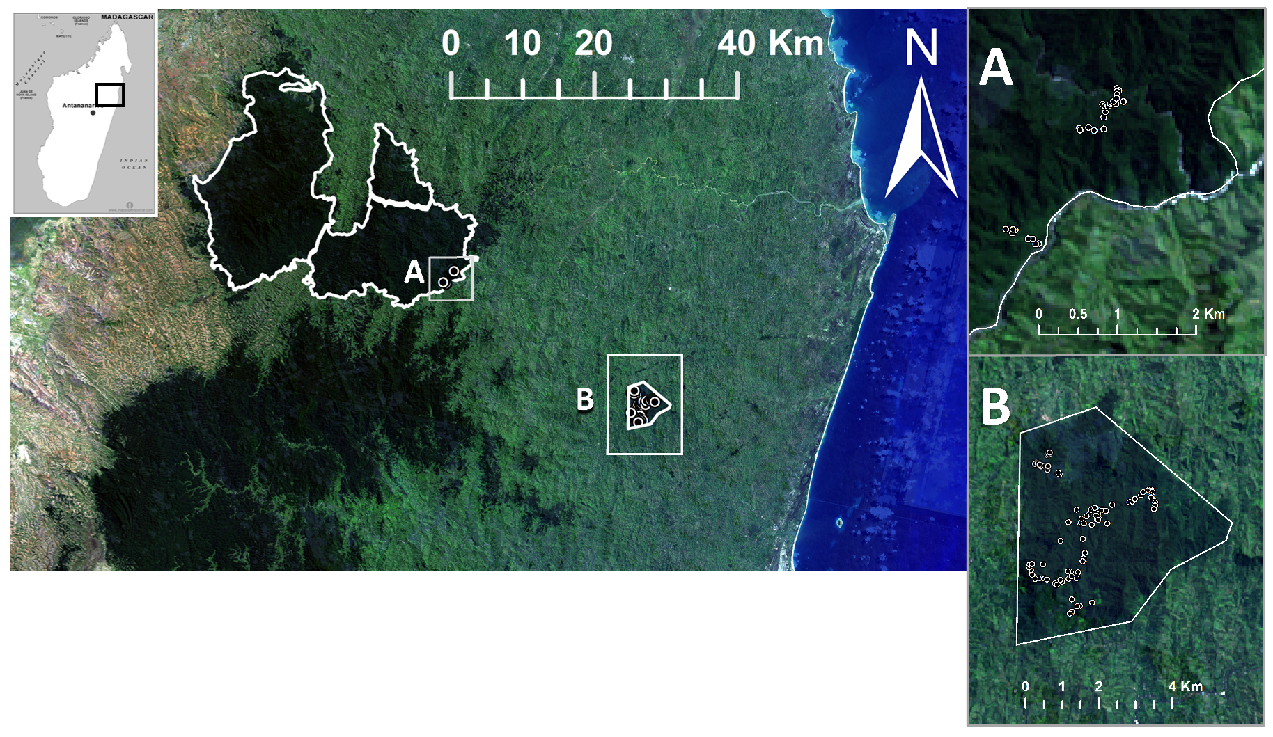
The model parameterization study site is Reserve Naturelle Integrale de (RNI) Betampona (translated: Betampona Strict Nature Reserve, henceforth referred to here as “Betampona” or “BTP”), a protected rainforest site in eastern Madagascar (
Figure 1). One of very few remaining tracts of primary lowland rainforest in the country [
23], Betampona is protected and only accessible through the acquisition of a research entry permit from the Malagasy government. Situated approximately 30 km to the northwest of the port town of Tamatave/Toamasina, the 2.23 km
2 reserve is located at 17°15′–17°55′ S, 49°12′–49°15′ E. Though given the protected status by the Malagasy government in 1927, enforcement was virtually absent until the 1990s. Based on conversations with the local organization managing Betampona’s protection, it is estimated that ca. 50% of Betampona (i.e., 1114 ha) is undisturbed primary rainforest, with an additional ca. 35% characterized as recovering primary lowland rainforest, and the remainder as secondary lowland forest. The inventory plots measured in this study were established in undisturbed and recovering primary lowland rainforest; no plots were located in secondary forest.
2.1.2. ZNP—Zahamena National Park, Madagascar
Zahamena National Park (ZNP) comprises a total area of 64.37 km
2, with 42.30 km
2 of National Park and 22.10 km
2 of Strict Nature Reserve (similar protection status as BTP, located at 17°37′45″ S, 48°43′30″ E). ZNP is isolated in an area of Madagascar that has virtually no infrastructure (roads, utilities, other facilities) and only little tourism. First established as a Strict Nature Reserve in 1927, its boundaries were amended a few times before the August 1997 Malagasy government decree that established its present-day boundaries. However, it was not until 2001 that ZNP achieved its current national park status [
24]. Because of its high biodiversity, 85% endemism, and disappearing ecosystem type, ZNP is one of the six national parks that comprise the “Rainforests of the Atsinanana”, which became a United Nations Educational, Scientific and Cultural Organisation (UNESCO) World Heritage Site in 2007 [
25,
26]. ZNP is approximately 30 km north-west of BTP, has a similar climate, and is believed to contain a similar floral community composition (There are currently no published studies that contain a full listing of the tree species in Zahamena National Park) (see
Supplementary A for more detail). The park comprises several rainforest ecosystems types, including lowland (where study plots were located), mid-elevation rainforest and mountainous rainforest. The study inventory plots were located on the eastern slopes of ZNP, in lowland rainforest.
Due to its isolated proximity and the political turmoil that Madagascar has experienced in recent decades, there is little or no enforcement of ZNP’s boundaries in terms of protection from encroachment, poaching, or burning (e.g., subsistence agriculture). In 2010, UNESCO designated the “Rainforests of Atsinanana” as “In Danger” [
27]. Currently, there is no published information on the state of the primary forest or how heavily the boundaries of ZNP have been logged or burned.
2.2. Inventory Dataset Collection
One hundred small (10 m-diameter) vegetation inventory plots were established in BTP in 2004. These plots were re-measured in 2005, and then fifty of these plots were re-measured for a third time in 2008. Because a GPS unit was not acquired in BTP until 2006, the plots were initially located in 2004 using a small hand-drawn map. A 1 km × 1 km grid was overlaid onto the map, whereby 15 full squares and 10 partial squares fell within the boundaries of the BTP, with an estimated 12 of the 15 full squares located in primary forest. Five plots were established at random locations within each full 1 km × 1 km grid square containing primary forest, with additional plots located in partial grid squares to total 100 plots. Plots were located at least 20 m into the forest off the main trail; however, steep terrain prevented this in some areas. Some plots were located closer to secondary trails. A multivariate statistical analysis that compared different aspects of species composition, size, and maximum height determined that the inventory plots measured near trails were not statistically different from plots measured farther from trails [
22]. A detailed description of the methodology used for plot location and measurement can be found in Armstrong [
22] and Armstrong et al. [
23].
In addition, thirty-five inventory plots of the same 10-diameter circular dimension were established in ZNP in 2008 (
Figure 1). The ZNP plots were established at random intervals along trails in lowland rainforest on a 20-day backpacking expedition that was led by a national park agent. All plots in ZNP were located at least 25 m away from the trail, as the trails in ZNP were slightly wider than the trails in BTP. Qualitative boundary descriptions to indicate location on slope, canopy gap effects, proximity to water, and GPS coordinates were recorded. Tree species were identified within each 10 m-diameter plot; in most cases, tree species identification was achieved through a local guide who is a resident expert on plant and tree species for the area. The same guide identified trees in both study locations. Species were recorded by Malagasy vernacular name. Scientific names were attained from the vernacular names by referencing Schatz [
28], consulting with non-government organization staff and botanists at the Missouri Botanical Garden (MBG) office in Antananarivo, Madagascar (see: [
22,
23] for a complete tree species list and detailed methods). When species could not be identified to the species level, genus only (and in one case family only) was recorded, with sp1, sp2, etc., used to denote individual unknown species of the same genus.
For all plots at both study sites, the following information was recorded for all tree ≥5 cm in diameter at breast height (DBH): species identification, DBH (cm), height (m), and presence of qualitative health characteristics such as bole wounding, disease, rot evidence, or strangling vines. When a tree was located at the plot border, if equal to or greater than 50% of the stem fell within the plot, the tree was counted as within the plot boundary. If less than 50% of the tree stem fell within the plot boundary, the tree was not counted as within the plot. When a tree was leaning or sprouting new growth after falling over, the DBH was measured at 1.37 m from where the trunk met the ground. When a tree split below DBH, each stem was measured at DBH as a separate tree. Standing dead trees were noted but not measured. Tree height was measured with a clinometer from a distance of at least 10 m (much larger in the cases of larger trees). All regeneration specimens with stems less than 5 cm DBH were identified and recorded for each plot. Finally, to obtain a sample of ground cover in the plot, a 1 m × 1 m square plot was randomly thrown from the plot center and all species of groundcover and regeneration smaller than having a woody diameter at breast height were identified and recorded.
2.3. The Forest Model FORMIND
Though the framework of individual-based gap models is perhaps the best-suited model type to simulate rainforest dynamics [
29,
30,
31,
32], few have been successful at achieving the persistence of the multitude of rarely occurring species, i.e., the immense biodiversity found in these forests, through space and time. The FORMIND model was developed specifically for the simulation of tree growth in tropical rainforests, by aggregation of tree species into plant functional types, and has been successfully applied to a larger number of sites [
17].
The spatial structure of the model is formulated in a similar manner to that of classical individual-based gap models [
2,
3,
6,
30,
33]. As the dominant driving factor of forest growth dynamics, competition for light and space occurs among the individual trees. Primarily, it is light climate that strongly influences the process of growth and also establishment; space competition is realized by the process of thinning, undergone when individuals die due to resource limitations brought on by crowding. Trees are simulated individually and each simulated tree belongs to a certain plot. Horizontally, the model sub-divides the one-hectare plot into 20 m × 20 m subplots, a size which roughly corresponds to the canopy spread of a mature canopy dominant tree [
3,
11]. In this way, all trees in one sample plot compete for light and space both vertically and horizontally. In addition, gaps formed by the death of a dominant tree can disrupt and influence growth in both the subplot where the gap formed, as well as adjacent subplots (see: [
11]).
The model is driven by the main processes of tree growth, competition for light and space, mortality, and regeneration. When a tree falls and a canopy gap is created, the vertical leaf distribution and light availability are calculated at the tree level. Biomass growth, also calculated at the tree level, is calculated as a balance of carbon based on photosynthesis, respiration, biomass allocation, and litter fall. Photosynthetic production is calculated as a function of the local available light (according to light response curves).
The basic structural framework of FORMIND follows the growth of individual trees while maintaining an overall balance of forest carbon on multiple levels. Forest growth in general is constrained by the photo-production of leaves, light climate within the different canopy layers, and loss of biomass through thinning or senescence. Competition among individual trees occurs for both light and space. As is a basic tenet of individual-based gap models, canopy gap formation caused by tree falls drives age, species, and canopy heterogeneity across the forest mosaic [
33]. A full listing of the equations that drive growth, photosynthesis, mortality, recruitment, and distribution dynamics in FORMIND can be found in Fischer et al. [
17]. Due to the individual- and process-based approach in FORMIND, it is possible to estimate forest stand productivity and respiration. Integrating carbon stocks for the deadwood and for the soil, FORMIND has the capability to simulate the full carbon balance of a forest stand [
18,
34,
35,
36]. In order to simulate the total ecosystem carbon balance, above- and belowground carbon stocks and the resulting net ecosystem exchange (NEE in tonnes C per ha per year) are calculated as the balance of carbon sequestration and carbon emissions (see [
17,
35] for a detailed description of the module).
2.4. Species Grouping into Plant Functional Types
In this study, we used two characteristics for grouping species into plant functional types (PFTs): shade tolerance and the potential maximum height of the tree. Following Whitmore [
15], we assumed three light demand classes, including: shade intolerant (pioneer species), shade tolerant trees (climax species), and intermediate shade tolerance. In addition, five canopy strata [
37]: emergent trees, main canopy, understory, woody treelets (saplings), and forest floor shrubs or small trees are layered into the model. The 244 tree species identified in Betampona study plots were classified based on information from literature [
28] and expert knowledge (botanists at the Missouri Botanical Garden Office in Antananarivo, Madagascar). The maximum height of each tree species was determined using the survey plot data, though in some cases, trees were assigned to a larger height class than suggested by field data, based on information from local botanists at the Missouri Botanical Garden Office in Antananarivo, Madagascar, the local guide, and conservations agents at Betampona, or observations of the species outside of the plot. Species that occurred in very low frequencies among survey plots and could not be identified beyond the family level of classification were left out of the model, but in total constituted less than 0.5% of the overall biomass found in the plots.
Because not all possible combinations of size and light class were found to exist in Betampona (e.g., shade intolerant forest floor herbs), species were divided among 12 total groups.
Table 1 (below) lists the size and light demand parameters for each group.
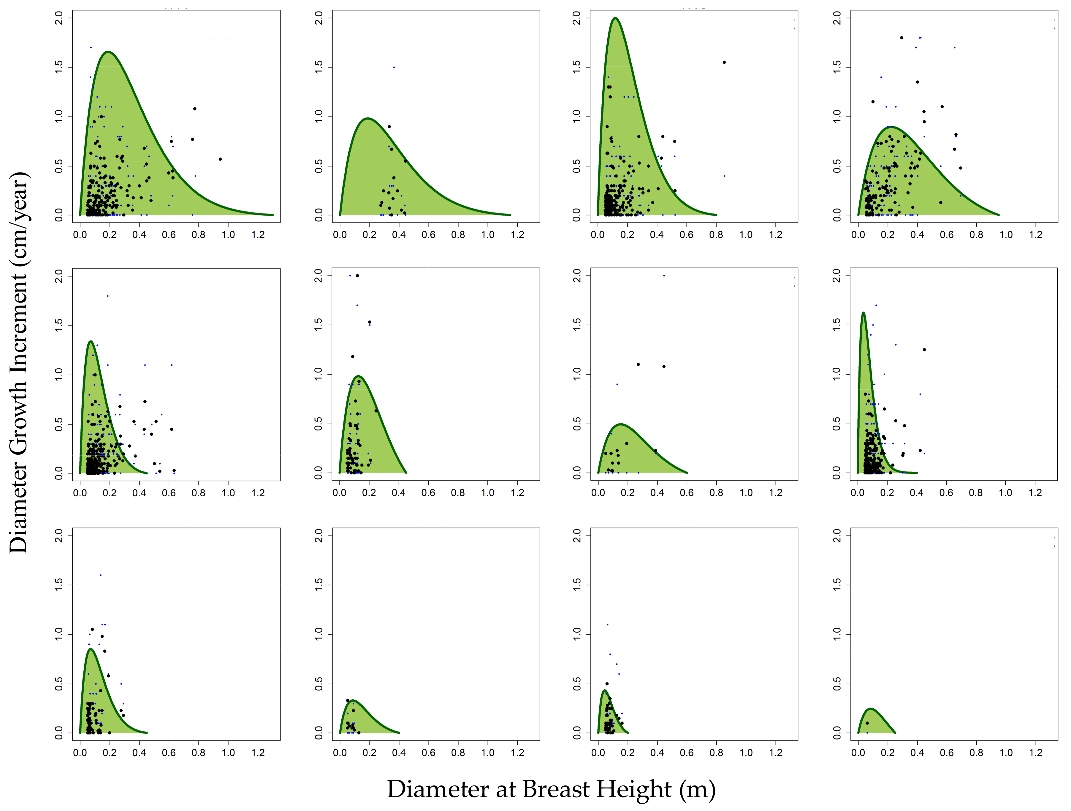
Figure 2 below shows the growth curve fitting for all 244 species found within the 12 PFTs. Growth curves were drawn from diameter growth increments (cm/year) and DBH (cm) for all individuals, the equations of which provided PFT-specific growth rate model parameters. Stem counts and the number of species that make up each group are included as derived from the survey plot data. A full species grouping list for Betampona (BTP) is documented in
Supplementary A. Similarly, the inventory dataset gathered in Zahamena National Park (ZNP) was divided into the FORMIND plant functional types that were derived for BTP as there were many overlapping species and a similar canopy structure. A full species grouping list for ZNP can be found in
Supplementary D.
2.5. Forest Model Parameters
All FORMIND model parameter values were taken from Fischer et al. [
38]. In Fischer et al. [
38], we used the FORMIX3 model (a predecessor of FORMIND) to estimate the impact of drought on lowland tropical forests in Madagascar (i.e., Betampona). In contrast to FORMIX3, the height stratification in FORMIND is more finely scaled and individual trees have a continuous height growth through time. In the current study, we adapted the FORMIX3 parameters that had been previously calculated for Betampona (BTP) to parameterize a new Madagascar rainforest version of the FORMIND model. Unknown parameter values (e.g., number of seeds) were determined with a calibration process by comparing the aboveground biomass, species composition, and tree density of a simulated mature forest with field data from the study region [
22,
23]. A description of the model parameters and their values can be found in
Supplementary B and [
38]. Following our parameterization and calibration of the FORMIND Model for BTP, we then validated FORMIND using another dataset that we collected in the lowland tropical rainforest of Zahamena National Park (ZNP). With the successful validation, our current study presents a FORMIND model version that can successfully simulate all lowland tropical forests within and around the study region.
2.6. Simulation Experiments and Validation
In this study, we used the FORMIND model to explore the forest dynamics of the investigated Malagasy forests. For the analysis of a mature forest, we simulated 50 hectares of forest succession over 1000 years starting with bare ground conditions. As this study did not focus on climate change, climate and soil conditions were held constant throughout all simulations. All calculated output values are mean values over the whole simulation area (50 ha) and over the last 500 years of the forest succession simulation, based on the assumption that the model in that period is in the equilibrium/climax state. In detail, we analyzed total stem numbers, aboveground biomass, basal area, and stem size distribution. We also analyzed gross primary production (GPP), respiration, biomass mortality, net primary production (NPP), and the stand carbon balance called net ecosystem exchange (NEE).
Though there are several definitions of NEE and NEP in recent literature, for our study, we defined NEE as the following (see: [
38]):
where GPP is the sum of the gross primary productivity of all the trees in the forest,
R is the total respiration of all of the living trees,
Rdead is the amount of carbon released from the deadwood pool to the atmosphere, and
Rsoil is the amount of carbon released from the soil carbon pool to the atmosphere. Thus, a positive NEE value indicates that the forest takes up carbon.
The simulation results were compared first between model output and the Betampona (BTP) forest verification dataset. For this comparison, only trees with DBH above 10 cm were included. To validate the FORMIND model for lowland rainforest in Madagascar, several simulated forest attributes were compared with the Zahamena (ZNP) dataset. Again, only trees greater than 10 cm DBH were included. The ZNP dataset was compared to both the model output and the BTP 2008 dataset, and the deviations of the two comparisons were analyzed. Further details and the results of this analysis can be found in
Supplementary A.
3. Results
Within the 100 BTP plots, a total of 233 tree species belonging to 49 families comprised the 2847 trees measured in 2004 and 2005 (1797 among 50 plots in 2008). Stems per plot ranged from 16 to 53 for trees (mean = 28.47) and 22 to 224 for regeneration (less than 5 cm at DBH; mean = 94.19), with an average of 19.27 species per plot in 2004. In addition, species per plot averages fell from 19.27 per plot in 2004 to 15.71 per plot in 2005. The per plot averages decreased in 2005 to 22.27 for trees and 57.28 for regeneration. For the plots measured in 2008, the average number of trees per plot was 35.94, with 54.1 stems of regeneration. However, there was an increase in the average DBH of trees from 12.77 cm to 13.5 cm. Similarly, both total plot basal area (m
2/ha) and average plot canopy cover (%) increased from 61.46 m
2/ha and 79% in 2004 to 81.51 m
2/ha and 83% respectively, in 2005. These trends are concurrent with dynamics that have been observed in other rainforests worldwide ([
16,
24]), where local thinning occurs following recovery from the formation of canopy gaps by large-scale disturbances such as cyclones, including Cyclone Kesiny, which heavily impacted the area in and around BTP in 2002.
3.1. Simulation of Forest Succession
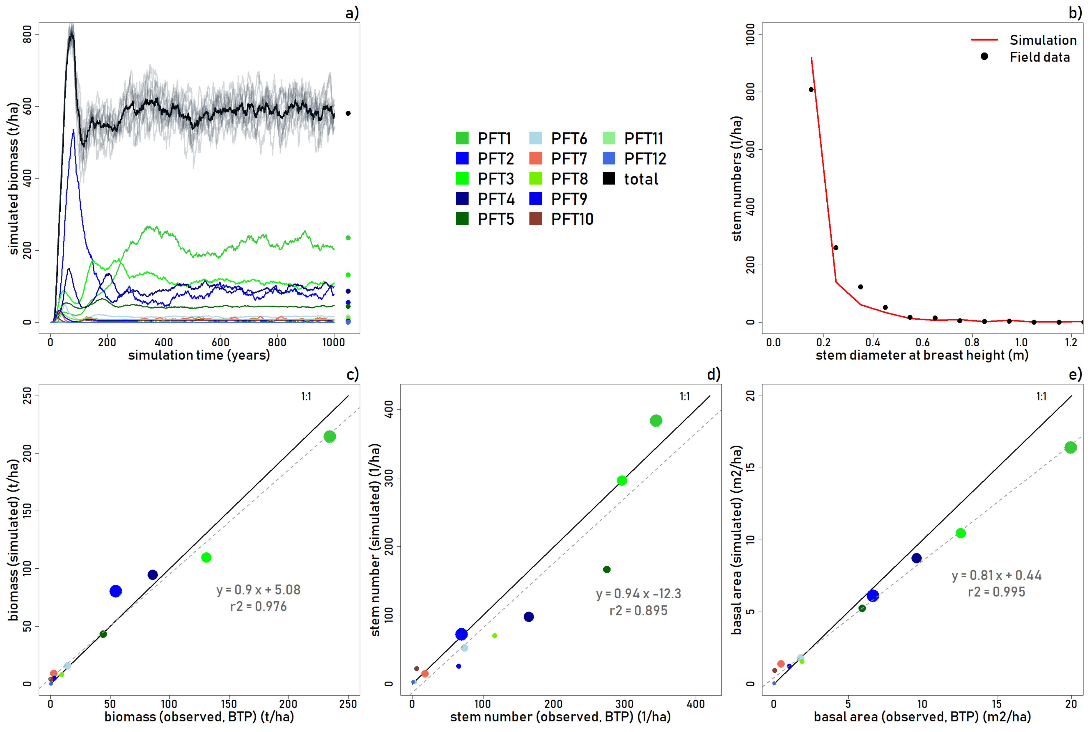
The life history of the simulated forests follows an ordinary successional pathway (
Figure 3a). Initially, the plot is colonized by small (PFT 10) and medium (PFT 7) shade intolerant trees, and small (PFT 9 and PFT 12) and large (PFT 2) intermediate tolerance trees, as well as an in-seeding of large shade tolerant trees. After the initial exponential increase in biomass, crowding leads to thinning and by year 50, shade intolerant PFTs 7 and 10, and intermediate PFT 9, are out-competed by larger intermediate and shade tolerant trees (PFTs 1 to 6). PFTs 3–6 have initial biomass peaks that thin by year 100. PFT 2 establishes as the dominant plant functional type, but peaks around year 100 when shade tolerant trees are thriving in closed canopy shadier conditions.
In year 200, canopy emergent and canopy shade tolerant classes (PFTs 1 and 3) dominate the overall biomass, while PFT2 and PFT4 are on the decline toward a more stable equilibrium. But in year 400, the forest reaches a climax state, dominated by large shade tolerant followed by intermediate tolerance tree species. From this stable equilibrium, small fluctuations of biomass occur following the deaths of large trees, and shade intolerant species colonize the gaps formed by treefalls (as seen by short peaks in biomass of PFTs 7 and 10) and are eventually out-competed or out-lived by intermediate or shade tolerant trees that colonize in the shady sub-canopy conditions.
The model accurately reproduces aboveground biomass (t/ha;
r2 = 0.976), stem numbers (
r2 = 0.895), and basal area (m
2/ha;
r2 = 0.995) for the BTP study site (
Figure 3a–e). The >10 cm simulated trees match well for the smaller statured plant functional types (PFT5-PFT12). Aboveground biomass in the simulation was slightly overestimated for the main canopy and emergent intermediate trees, and slightly underestimated for the main canopy and emergent shade tolerant trees.
As shown in
Figure 3b, the model slightly overestimates the number of trees 0.2 m-DBH and less, but underestimates the number of trees between 0.25 m and 0.5 m-DBH. This is further explained in
Figure 3d, which shows stem number as overestimated in the simulation for PFT 1, and underestimated for PFTs 4, 5, 6, 8, and 9. Basal area was slightly underestimated in the simulation for PFTs 2 and 4. The slightly low aboveground biomass and basal area but inflated simulated stem numbers for PFT 1 suggest that the model grows a larger number of comparatively smaller shade tolerant canopy emergent trees (in terms of maximum size) than was measured in BTP. Overall, however, the results show that the model reproduces the main forest structural patterns observed in the BTP plots with respect to aboveground biomass, stem numbers, and basal area (
Figure 3c–e).
3.2. Comparison of Model Simulations with Independent Field Data
Following the model verification to the BTP forest inventory dataset (see
Supplementary C), we compared the FORMIND model simulation to the ZNP forest as a model validation test site. While the character of ZNP forest differs slightly from BTP (see
Supplementary A), the simulated forest approximates the structure of the ZNP forest overall, with per PFT stem counts per hectare, aboveground biomass (Tonnes C/ha), and basal area (m
2/ha)
R2 values of 0.95, 0.96, and 0.963 in 1:1 correlations, respectively (
Supplementary A). The overall biomass falls within the runs and there is strong agreement with respect to the largest tolerant and intermediate tolerance shade classes.
The most significant divergence in terms of forest structure occurs in the model’s underestimation of the overall stem numbers and basal area (m
2/ha); the aboveground biomass does not differ significantly. This is primarily due to the underestimation of stem numbers of sub-canopy and woody treelets by the model (PFTs 5, 6, 8, and 11). Basal area for large intermediate shade tolerance (PFT 2 and 4) trees was slightly overestimated by the model, but the degree was not significant enough to offset the overall underestimation (
Supplementary A). Similarly, the largest shade tolerant group (PFT 1) and PFTs 2 and 4 were also overestimated by the simulation.
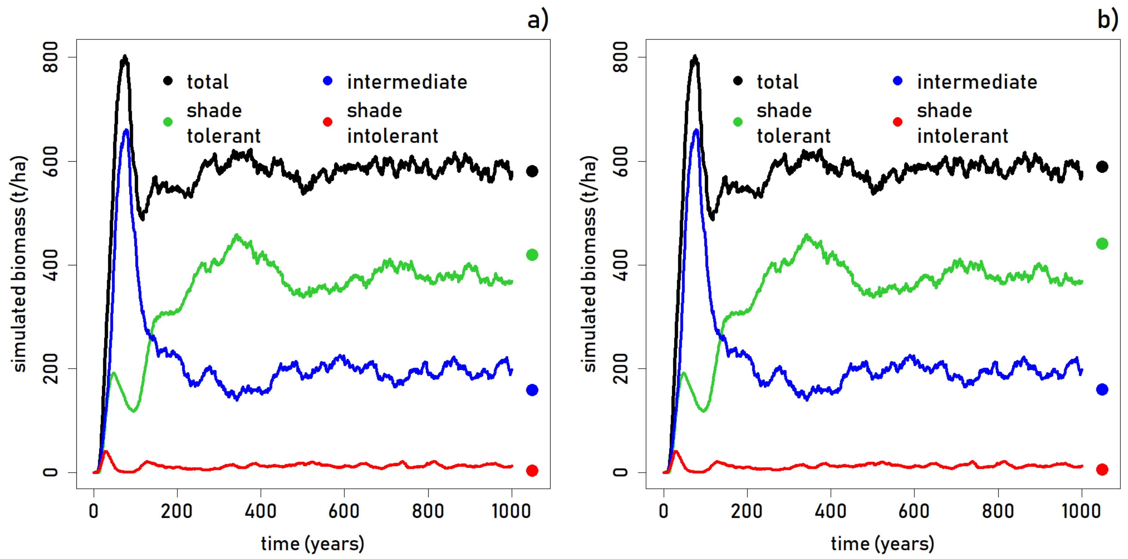
To assess the differences in the comparative accuracies through time,
Figure 4 shows successional groups related to light requirements for BTP and ZNP. It is interesting to note that there are relatively few shade intolerant trees overall in the forest, but especially in the initial colonization of the forest simulation. Initially, only a small number of shade intolerant trees colonize the bare ground, and the overwhelming majority of the biomass is from intermediate tree growth. In both forests (
Figure 4), shade tolerant trees are underestimated by FORMIND, but both are within the margin of the range in biomass seen throughout the simulation. Intermediate trees are overestimated at both sites, though the simulation numbers do match the field numbers at around year 375 of the simulation, when shade tolerant trees account for the highest percentage of biomass and intolerant trees are at their lowest. However, these forests are both very old and have not been clear-cut in the past 400 years. Rather, the cause is more likely that a number of species were placed in the wrong plant functional groups.
3.3. Forest Productivity
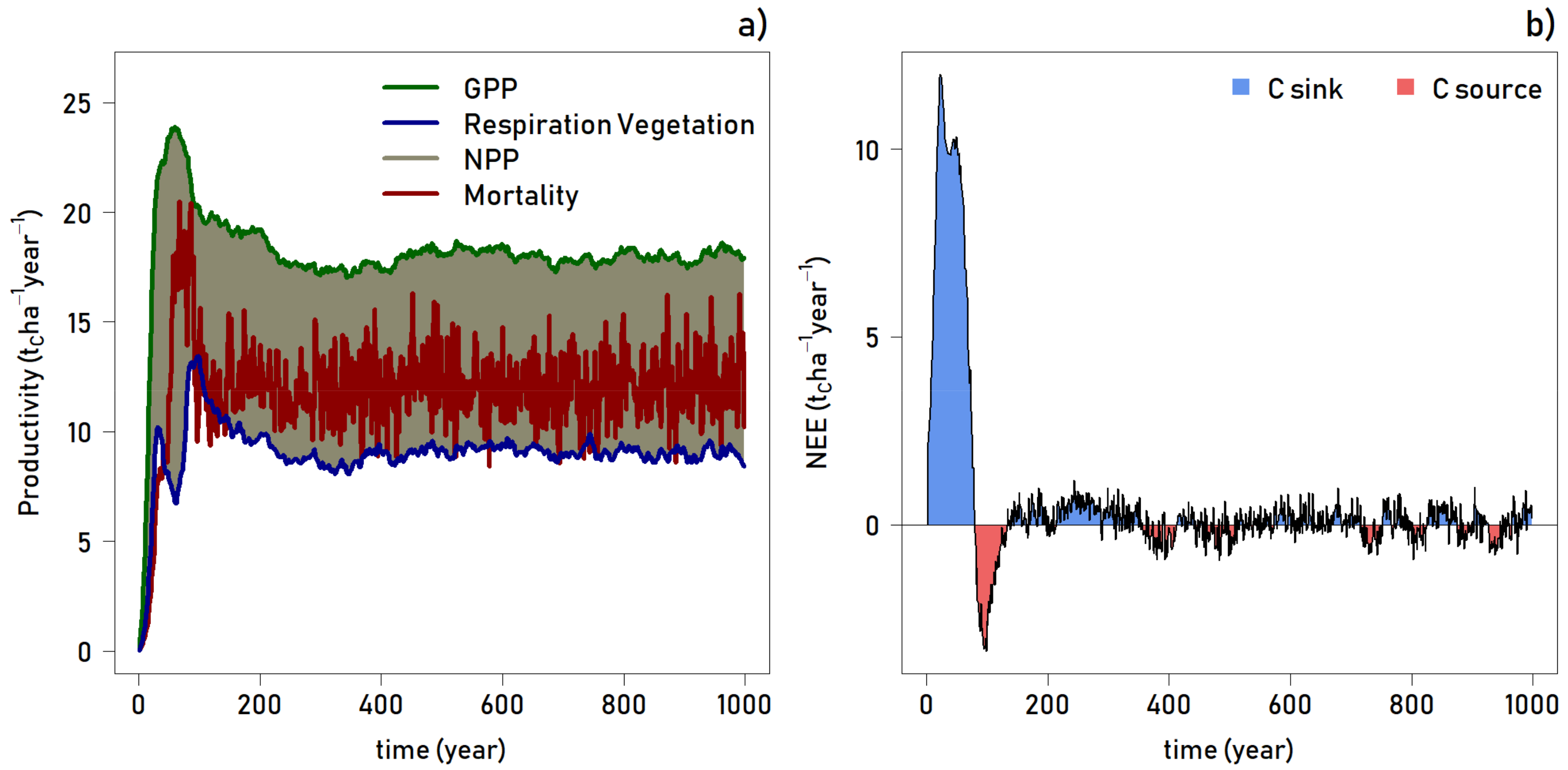
A time series analysis of net primary productivity (NPP), plant respiration, gross primary productivity (GPP), and tree mortality reveals an expected pattern through time (
Figure 5, top). After the initial exponential increase in productivity in the first 25–30 years, there is a sharp decline in respiration and a spike in mortality, as the young forest stand undergoes initial competition and thinning. By year 60, respiration has reached a low, while GPP is peaking; NPP is highest as dominant trees quickly grow into a closed canopy forest. At this point, mortality is also on the rise due to the forest thinning and competition for resources. At about year 100, plant respiration reaches a second peak, where GPP is declining, thus NPP is the lowest during the entire simulation, and mortality is high. Following successional dynamics, growth has slowed as the canopy has closed, there is dieback of the out-competed individuals, and pioneer species are being replaced by intermediate and climax species. By approximately year 250, the forest reaches an equilibrium with respect to productivity (
Figure 5, top).
Related to productivity, carbon flux is an important measurement used to classify the contribution of an ecosystem to the global carbon cycle. As shown in
Figure 5, the net ecosystem exchange (NEE; in tons of carbon per hectare per year) indicates that the forest switches from a carbon sink to a carbon source after 75 years. During the thinning stage as described above, the forest emits carbon to a maximum of about 3.5 t Cha
−1 year
−1 in year 95. By year 130, the forest once again becomes a carbon sink, and for the remainder of the 1000 simulation, the forest fluctuates between sink and source. The NEE values are very small and range between 1 and −1 t Cha
−1 year
−1, consequently the forest can be considered as a net neutral or a very slight carbon sink ecosystem from year 130 to year 1000.
4. Discussion
In this study, we applied the forest model FORMIND to simulate the dynamics of Madagascar lowland rainforest in Reserve Naturelle Integrale de Betampona, and then validated FORMIND in the lowland rainforest of Zahamena National Park. Madagascar, known for its >80% endemicity, is a imperilously threatened global biodiversity hotspot [
39]. With the diminishing forest resources, the need to effectively conserve the remaining ecosystems has been eclipsed by the lack of long term inventory datasets, and there are few studies devoted to how the remaining forests and forest fragments will survive under the anthropogenic threat and changing environmental conditions. Our model has the ability to evaluate and simulate scenarios involving changing climatic conditions [
38] and has been applied to a number of other tropical forests worldwide for understanding how the structure and dynamics are altered in fragmented forests [
18].
A general challenge of predictive forest modeling is to accurately simulate and subsequently forecast how forest stands will develop in the near and distant future in response to the many disturbances to which they can be subjected, including: fragmentation, fires, logging, pollution, the loss of pollinating and seed-dispersing animals, and the direct (leaf physiology) and indirect (climate) effects of increasing atmospheric CO
2 [
40]. An important advantage of the application of individual-based models (IBMs) toward understanding the impact of such perturbations is that their framework allows the modeler to control the resolution at which they are studied, both spatially and temporally [
13]. Shifting dynamics be studied on the scale of individual leaf-level changes up to landscape scale, and IBMs like FORMIND have been extensively applied with field data from various tropical forests [
11,
13,
18,
38,
41,
42,
43].
Our Madagascar FORMIND Model accurately simulated the structure of both BTP and ZNP forests, though a few features of each were not well captured by the forest simulation. For instance, as shown in
Figure 4 and
Figure 5, simulated total aboveground biomass and stem counts per PFT matches our calculations from field data well in the case of Betampona, and is within the range seen across the 50 runs, for the case of Zahamena. However, in looking at the stems per diameter size class for each (
Figure 4 and
Figure 5), it is clear that the model underestimates the number of smaller to medium trees as compared to both study site datasets. At both sites, the smallest size (10–20 cm DBH) was overestimated by the model. Thus, though FORMIND is accurately depicting the forest structure in general, the character of the forest appears slightly differently. In BTP and ZNP, there are fewer small trees and more mid-sized trees.
Two notable sources of error that occurred with the development of our parameterization were: (i) so little is known about Madagascar tree species in general, that the placement of species in the proper plant functional type groups was very challenging; and (ii) the growth forms of trees in Madagascar forests are not consistent with other rainforests worldwide. With respect to the first issue, the dataset used to parameterize this forest model contains a number of tree species that are described only to the genus level at present. The maximum sizes and light requirements of many of these species are not definitively known, thus their group placement was an educated guess based on expert knowledge and field-based observations. It is therefore likely that as more is learned about the tree species that occur in RNI Betampona, the placement of species into plant functional groups may be improved.
Figure 4 shows that the model consistently overestimates aboveground biomass for intermediate shade tolerance species, but underestimates it for shade tolerant species, for both BTP and ZNP forests. In addition, a strong May cyclone (Kesiny) caused damage to Betampona and Zahamena in 2002. The recovery from this cyclone would still be occurring within the forest in 2004, 2005, and 2008. While the foliage would have recovered by 2004, large limbs and large trees downed in this storm would have initiated gap dynamics and could have slightly affected growth curves for smaller trees undergoing release from light suppression.
A notable feature (see [
23]) observed during the plot survey, the high abundance of palms, pandans, and tree ferns in Madagascar rainforests, could explain a significant proportion of the error exhibited by the FORMIND simulation with respect to growth within diameter classes (
Figure 3c). The high importance (#2) of the Malagasy traveler’s palm,
Ravenala madagascariensis, as well as other palms and members of the
Pandanaceae family, could account for some of the discrepancies that occurred in both the biomass and basal area calculations due to their atypical growth forms (
Figure 4 and
Figure 5). In comparison to the other forests that FORMIND has been successfully parameterized for, RNI Betampona has a highly significant proportion of trees with non-phanerophytic growth forms. It is possible that a source of error with respect to the growth and maximum sizes of trees is that the ability to capture anomalies such as atypical growth forms is diminished when tree species are aggregated into functional groups.
Madagascar lowland rainforest has among the highest species diversity per hectare in the world [
23]. Aboveground biomass was found to be high, more akin to Malaysia and Papua New Guinea [
44] than to Amazonian [
45,
46,
47,
48,
49,
50] or African [
51,
52] forests.
Forests are primarily thought of as carbon storage pools within the global Carbon cycle. Research suggests that particularly in the tropics, though forests are typically carbon sinks, they can act as a carbon source during certain periods within their lifecycle (e.g., self-thinning). The FORMIND model executes growth on a carbon balance and records carbon flux throughout the simulation. With respect to NEE, Grace et al. [
53] found undisturbed forest in southwest Amazonia to store 1.02 t Cha
−1 year
−1. Grant et al. [
54], found their study site in Tapajo’s National Forest (TNF) in Para, Brazil, to be within 100 g Cm
−2 year
−1 of net neutrality in the absence of major disturbance. Their study also noted that rainforests can range from moderate C sinks (1.0 t Cha
−1 year
−1; [
54]) to those large in size (3.0–7.0 t Cha
−1 year
−1; e.g., [
55,
56,
57,
58]); but that some studies conducted in their study area were found to be C sources ranging from (~0.8–~1.9 t Cha
−1 year
−1 [
59,
60]). Our simulation resulted in a time series range of values averaging between +1.0 and −1.0 t Cha
−1 year
−1, indicating that Madagascar lowland rainforest is as highly productive as it is diverse.

 ,
, 


