Article

Influences of Extreme Weather Conditions on the Carbon Cycles of Bamboo and Tea Ecosystems

1
Key Laboratory of Watershed Geographic Sciences, Nanjing Institute of Geography and Limnology, Chinese Academy of Sciences, 73 East Beijing Road, Nanjing 210008, China
2
School of Forestry and Environmental Studies, Yale University, New Haven, CT 06511, USA
3
Yale-NUIST Center on Atmospheric Environment and Collaborative Innovation Center on Forecast and Evaluation of Meteorological Disasters, Nanjing University of Information Science and Technology, Nanjing 210044, China
*
Author to whom correspondence should be addressed.
Forests 2018, 9(10), 629; https://doi.org/10.3390/f9100629
Submission received: 30 August 2018 / Revised: 8 October 2018 / Accepted: 9 October 2018 / Published: 11 October 2018
(This article belongs to the Section Forest Ecology and Management)

Abstract

:
Tea plantations have expanded rapidly during the past several decades in China, the top tea-producing country, as a result of economic development; however, few studies have investigated the influence of tea plantations on the carbon cycle, especially from the perspective of climate change and increases in extreme weather events. Therefore, we employed combined observational and modeling methods to evaluate the water and carbon cycles at representative bamboo and tea plots in eastern China. Green tea growth and the corresponding water and carbon cycles were reproduced using the Community Land Model after applying fertilizer. Old-growth bamboo was reasonably simulated as broadleaf evergreen forest in this model. The mean observed soil respiration ranged from 1.79 to 2.57 and 1.34 to 1.50 µmol m−2 s−1 at the bamboo and tea sites, respectively, from April 2016 to October 2017. The observed soil respiration decreased by 23% and 55% due to extreme dryness in August 2016 at the bamboo and tea plots, respectively, and the model reproduced these decreases well. The modeling results indicated that tea acted as a stronger carbon sink during spring and a stronger carbon source during autumn and winter compared with old-growth bamboo. The carbon cycle was affected more by extremely dry weather than by extremely wet weather in both the bamboo and tea plots. Extremely dry periods markedly reduced the carbon sink at both plots, although this trend was more pronounced at the tea plot.

1. Introduction

Tea is the second most consumed beverage in the world and is one of the “business cards” of Chinese culture. Driven by economic development and the rise in living standards, tea plantations have expanded rapidly over the past several decades in China. China currently has the largest area of tea plantations and produces the most tea in the world, accounting for approximately 60% and 50% of the world’s plantations and production in 2016, respectively [1]. The area of plantations in China is currently around 30,000 km2, which increased by 143% from 2000 to 2014, representing the most rapid increase worldwide [1]. Moreover, tea production is predicted to increase by 55% from 2013 to 2023 [2]. This rapid expansion in tea plantations must be achieved by reducing the area of other land types, in most cases causing deforestation, because tea is usually planted in hilly areas in China. However, few studies have investigated the influences of tea plantations and corresponding land use changes on the terrestrial carbon (C) cycle.
Climate change and extreme weather and climate events (EWCEs) have increased the complexity of the influences of tea plantations on the terrestrial C cycle. EWCEs occur frequently in the middle and lower reaches of the Yangtze River (MLRYR), where water resources are plentiful and the monsoon climate is dominant. For example, the entire Yangtze River experienced the second largest recorded flood in the 20th century in 1998. Meanwhile, the MLRYR suffered from a drought with a return period of 50 years during the spring of 2011 [3] and experienced another severe flood in 2016 accompanied by rainfall from June 19 to July 20 equivalent to twice the multi-year average (600 mm) [4,5]. Increasing frequencies of extreme rainfall events [6,7,8,9] and extreme droughts [10,11,12,13] have been projected with increasing global air temperature. Tea plantations located in the southern region of the MLRYR produce more than two-thirds of the tea in China [14] and are frequently affected by EWCEs; however, no studies have assessed the influences of EWCEs on the C cycle in tea plantations.
Bamboo is another plant with special meaning in Chinese culture; for example, a man of complete virtue is often compared to bamboo in China. Bamboo forests account for 2.97% of the total forest area in China [15] and have a similar spatial distribution as that of tea in China (e.g., in Zhejiang, Fujian Province) [16]. As a result, tea plantations are often developed at the expense of bamboo forest (e.g., at the present study site). Currently, the area of tea plantation is approximately half that of bamboo forest [15]. In recent years, bamboo has received attention for its high capacity to store C and potential for C farming and trading [16,17]. Therefore, the influence of replacing natural bamboo forest with tea plantations on the C cycle must be investigated in depth.
The tea plant can be categorized as a shrub (shorter varieties) or tree (taller stages or varieties), and fertilization is required to increase production. However, most land surface models do not have an option or module for fertilized shrubs or trees in agroforestry, including the most widely used land surface model in climate change studies, the Community Land Model (CLM). Meanwhile, bamboo is biologically classified as a giant grass [18], although its height, stem, and other characteristics are tree-like. To our knowledge, no studies have assessed the performance of the CLM in modeling bamboo.
In this study, we monitored meteorological indexes and soil water content and measured soil respiration (SR) at a reference bamboo plot and a green tea plot in Taihu Basin, MLRYR. Then, we constructed and validated mathematical models based on the field observations and data from the literature. We aimed to evaluate the performance of the widely used CLM model in modeling the growth and C cycles of bamboo and tea ecosystems, to analyze the complete C cycles in these two plots, to investigate the influences of land use change from moso bamboo to green tea on the C cycle, and to investigate the influences of extreme weather and climate events on the growth and C cycles of these two ecosystems.

2. Materials and Methods

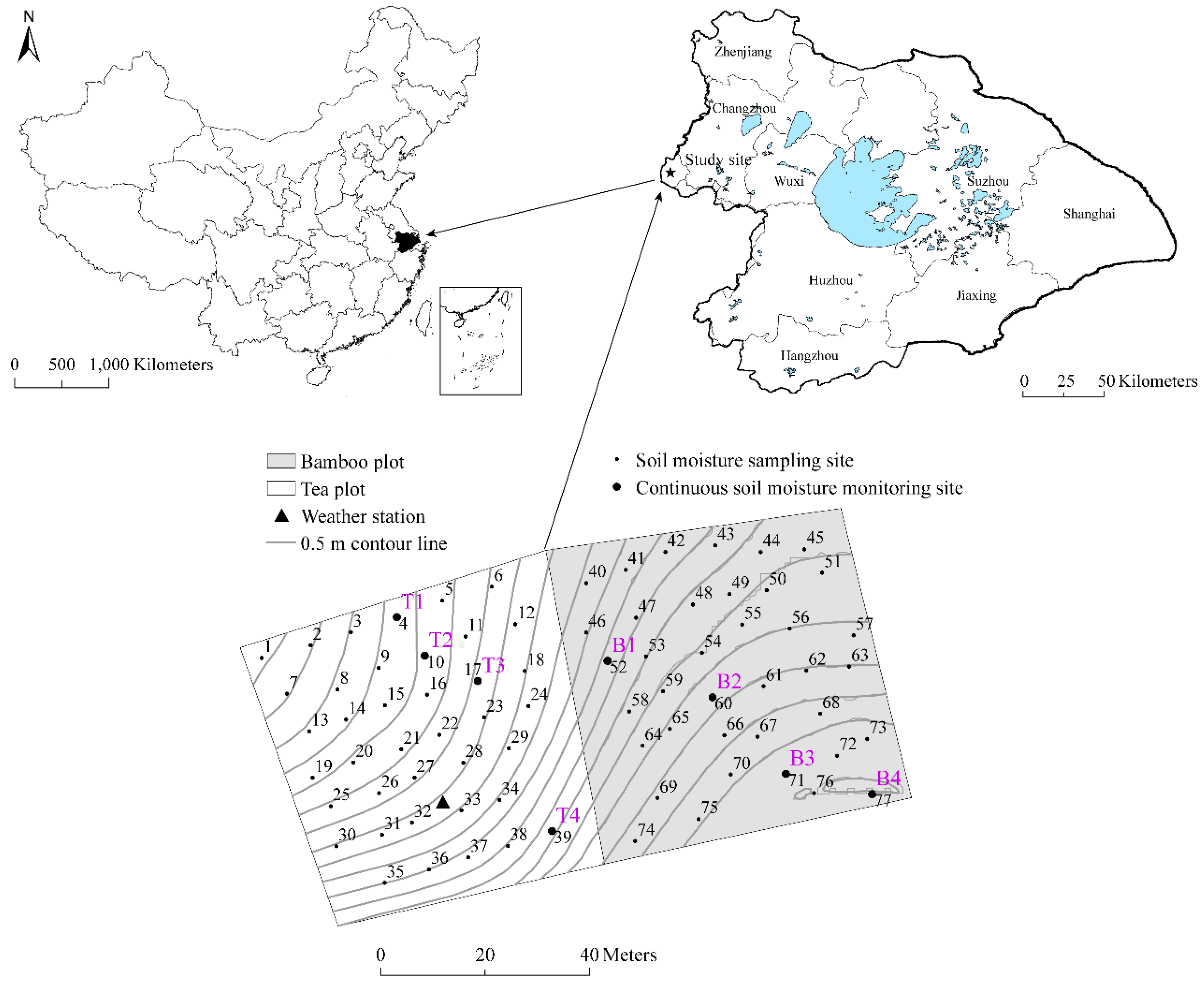
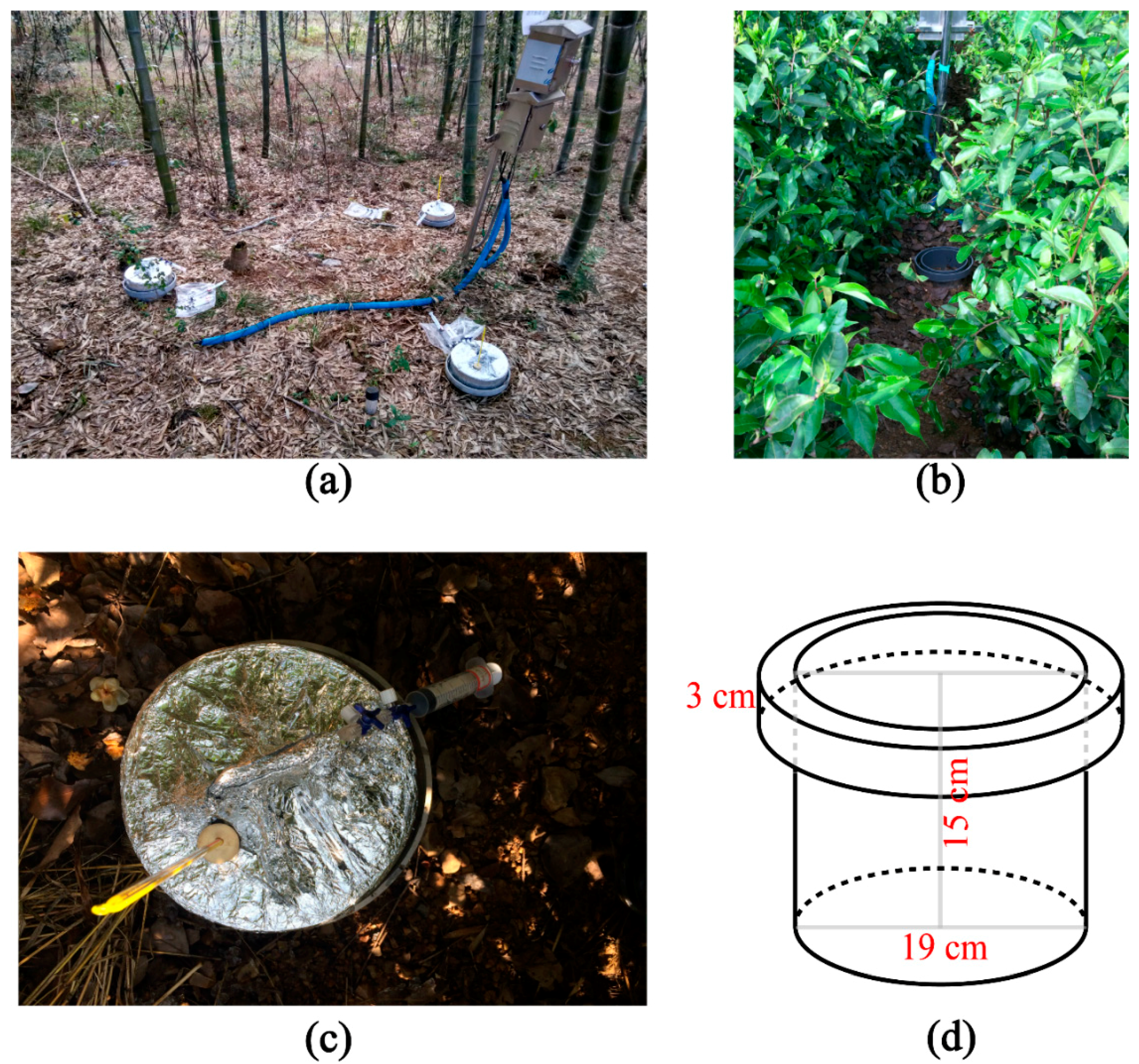
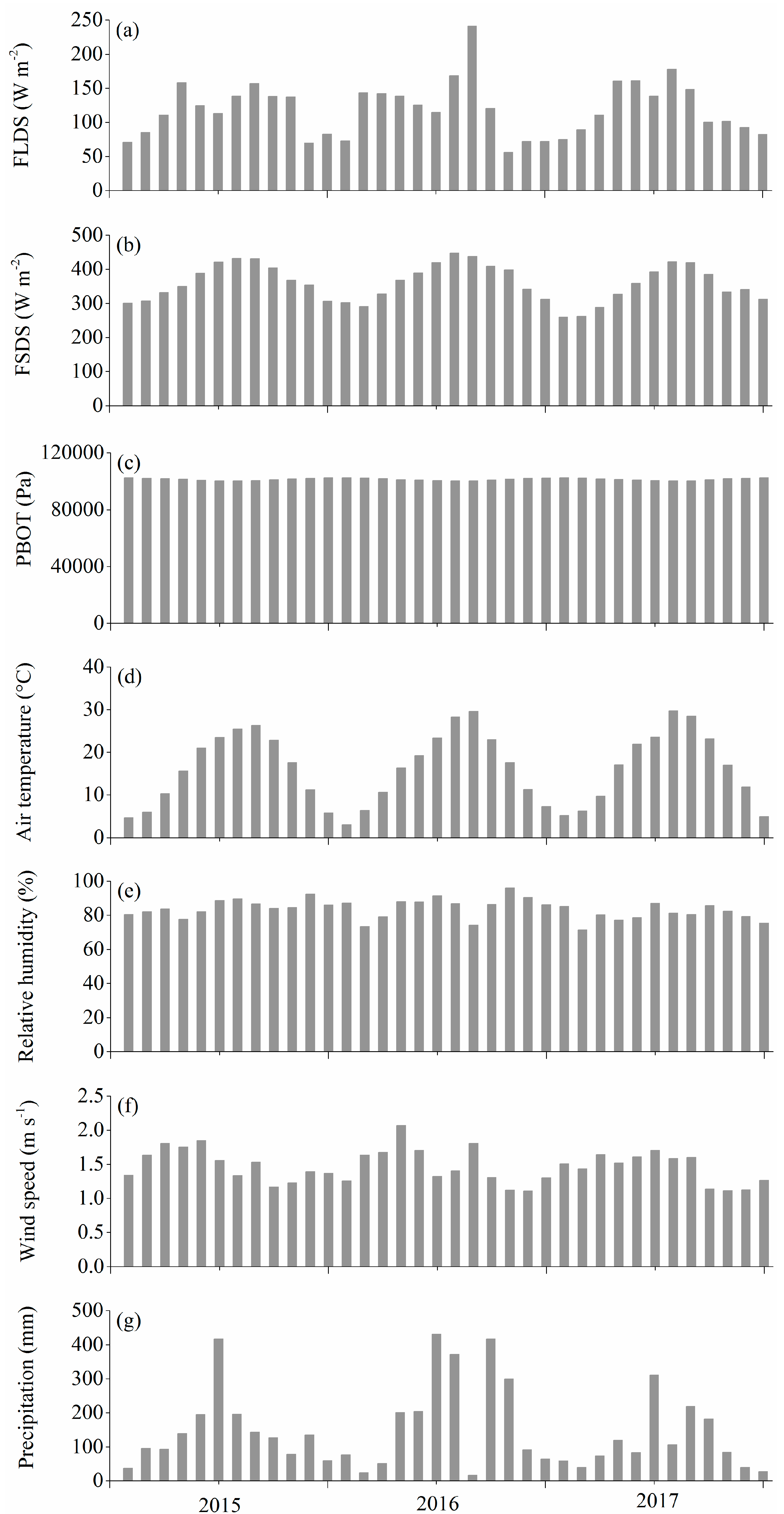
2.1. Study Sites and Data

This study was conducted at an experimental hillslope site (31°21′ N, 119°03′ E) in Taihu Basin, eastern China, which is part of the MLRYR and is located approximately 230 km west of Shanghai (Figure 1). The study site has a north subtropical–middle subtropical transition monsoon climate with a mean annual precipitation of 1157 mm and a mean annual temperature of 15.9 °C (2006–2016). The study site includes a moso bamboo (Phyllostachys edulis (Carr.) H. de Lahaie) plot and a green tea (Camellia sinensis (L.) O. Kuntze) plot (Figure 1). Bamboo, tea, and mixed forest are the dominant plants at the study site. Moso bamboo accounts for 34% of the forest in Taihu Basin [19]. The bamboo forest in the present study is under near-natural conditions and is at the old-growth stage (>20 years old; Figure 2a). The rapid biomass and C accumulation of newly planted bamboo was not within the scope of this study. As described in Section 1, the MLRYR accounts for two-thirds of tea production in China, and the green tea analyzed in the present study represented the dominant tea type in China [1].
The hillslope at the study site has a slope of 0%–21%, and the mean slopes of the bamboo and tea plots are 8.5% and 11.5% [20,21], respectively. The soil texture of the two study sites is silt loam with a mean silt content >70%. The depth from the surface to the soil–bedrock interface varies from <0.3 m to around 1.0 m, and the mean depths at the bamboo and tea plots are 0.56 m and 0.49 m [22], respectively.
An automatic weather station (see location in Figure 1) was installed to collect and record incoming solar radiation, rainfall, air temperature, relative humidity, and wind speed in 5-min intervals. Data from a nearby state meteorology station, Yixing station (31°20′ N, 119°49′ E), a nearby airport weather station (31°45′ N, 118°52′ E), and National Centers for Environmental Prediction (NCEP) reanalysis data with a resolution of 1.905° × 1.875° (only incoming longwave radiation in 2017; ftp://ftp.cdc.noaa.gov/Datasets/ncep.reanalysis) were used when the corresponding instruments of the automatic weather station were non-functional, or relevant data were unavailable (Figure S1).
The volumetric soil water content used in the present study (1 January 2015 to 31 December 2017) was monitored continuously and recorded in 5-min intervals using EC-5 SWC sensors (Decagon Devices Inc., Pullman, WA, USA) at six sites in the bamboo (points B1, B2, and B4 in Figure 1) and tea (points T2, T3, and T4 in Figure 1) plots. One to three sensors were installed at depths of 5, 10, and 30 cm at each site, and the soil water content was also monitored at a depth of 40 cm at the bamboo plot (Table 1). The EC-5 sensors were calibrated using a portable time-domain reflectometry TRIME-PICO-IPH probe (IMKO Micromodultechnik, Ettlingen, Germany) for each site and soil depth [23].
SR (heterotrophic respiration (HR) + root respiration (RR)) was measured from bimonthly to monthly from 13 April 2016 to 18 October 2017 using the closed chamber technique [24]. For the gas flux measurements, a series of three aluminum unvented chambers (open bases of 50 cm × 50 cm × 30 cm) at each site (bamboo plot: B1–B4; tea plot: T1–T4) were inserted into the soil to a depth of 15 cm to ensure an airtight seal and left throughout the cropping cycle (Figure 2c,d). Gas sampling was normally carried out between 09:00 and 11:00, which was assumed to be representative of the daily mean [24]. The modeling results supported this assumption, with a difference of less than 7% between the daily and mean values between 09:00 and 11:00 (see Section 3). To ensure adequate mixing of air within the chamber, the chamber air was mixed using a 60-mL syringe before sampling, and four gas samples were taken from each chamber headspace (0, 10, 20, and 30 min after closure) using a 30-mL syringe (Terumo, Tokyo, Japan) for transport back to the laboratory. Three samples were taken at each site at each sampling time. Carbon dioxide (CO2) concentrations in the gas samples were analyzed in the laboratory using a gas chromatograph (Varian 3800). The SR (CO2 flux) FCO2 (µmol m−2 s−1) was calculated as follows:
F C O 2 = ρ h 273 273 + T d C d t 3.788
where ρ is the density of CO2 (g cm−3), h is the height of the closed chamber from the soil surface (cm), T is the air temperature in the chamber (°C) measured using a thermometer (Figure 2c), C is the measured CO2 concentration in the gas samples (ppm), t is time (10 min in this study), and 3.788 is a unit conversion factor.

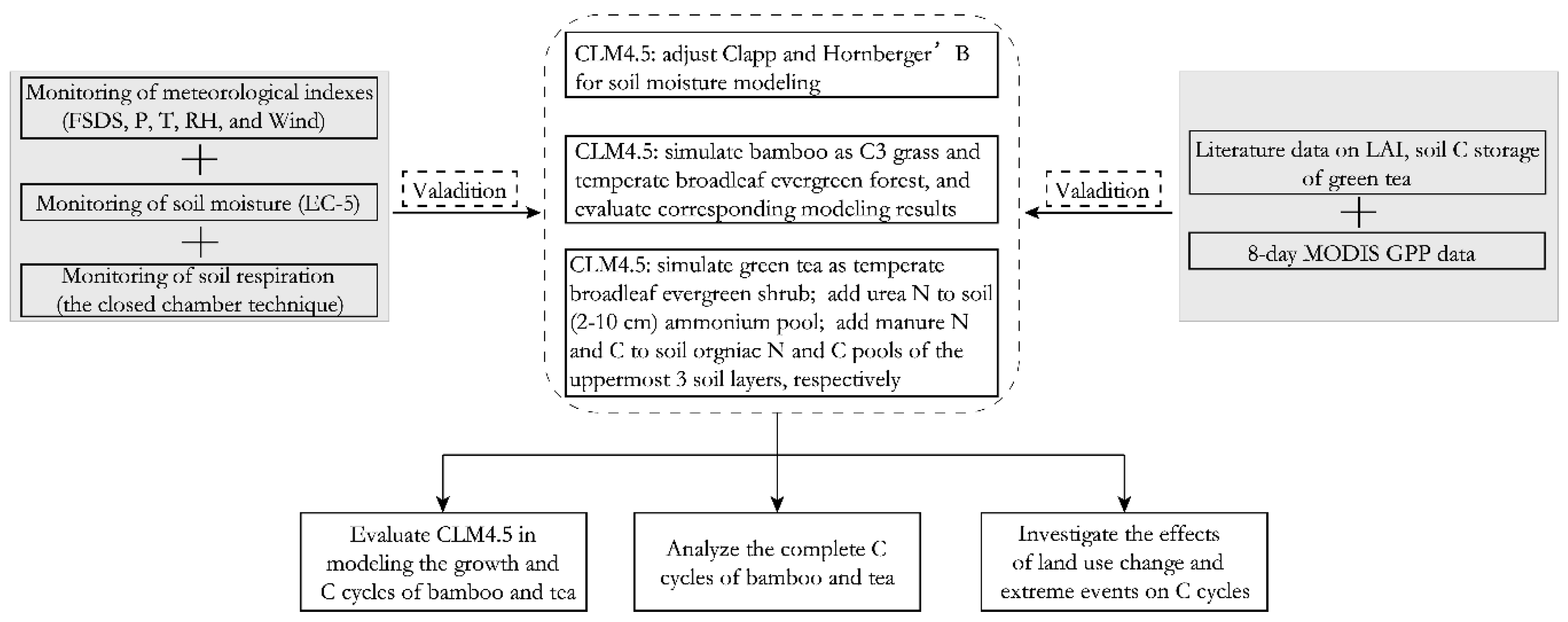
2.2. Land Surface Model

CLM ver. 4.5 (CLM4.5) [25] was used to simulate plant growth, water, and the C and nitrogen (N) cycles for the two ecosystems in this study. In CLM4.5, water, C, and N flux models are based on the offline ecosystem process model Biome-BGC ver. 4.1.2 [26,27,28]. The CENTURY-based soil C pool kinetics (CLM45BGC) [29] in CLM4.5 was used in the present study. The soil–water content simulation in CLM was based on the one-dimensional Richards equation. The air forcing data used to drive the model included air temperature at a height of 2 m, precipitation, wind speed, relative humidity, surface atmospheric pressure, incident solar radiation, and incident longwave radiation (Figure 3 and Figure S1). The single-point mode of the CLM model was used for each plot.
Green tea plants are usually fertilized in China; therefore, urea and manure were applied to the tea plot. Specifically, 209 and 174 kg N ha−1 were applied in the form of urea on 16 March and 30 October of each year, respectively, and 120 kg N ha−1 and 1792 kg C ha−1 were applied as manure on 30 October. CLM4.5 currently has simulation options available for corn, soybean, and cereal, but no option or module exists for green tea. In this study, green tea was treated as temperate broadleaf evergreen shrub, and we added N fertilizer to the soil ammonium pool and added C to the first soil organic C pool on the corresponding application dates by revising the source codes for the C and N cycles. Specifically, urea N was added to soil layers at a depth of 2–10 cm by revising the N state update procedure in the CLM (CNNStateUpdate1Mod.F90), in which fertilizer was added to the ammonium pool in the default CLM for corn simulations. Manure N and C were added to the first soil organic N and C pools of the uppermost three soil layers for the tea plot, respectively. To determine the optimal method to simulate bamboo growth, we compared simulations in which bamboo was treated as either C3 grass or temperate broadleaf evergreen forest.
Soil water dynamics reflect the comprehensive influences of rainfall, evapotranspiration, and lateral leaching; therefore, we used the soil water content to validate the modeling results for the water cycle. In our previous C/N modeling studies based on CLM4.5, CLM4.5 roughly captured the net ecosystem exchange (NEE) dynamics at a site in Minnesota representing the United States Corn Belt, a Douglas fir site in Washington State, a Mesquite Savanna site in Arizona, an oak pine forest site in southern California, and an Amazon evergreen forest site in Brazil [30,31]. Moreover, CLM4.5 reproduced gross primary production (GPP), net primary production (NPP), soil organic C content, and litter and fine root masses [31]. A cumulative 8-day MODIS GPP product with a pixel size of 500 m (MOD17A2H version 6) was provided by Running et al. (2015; https://lpdaac.usgs.gov/dataset_discovery/modis/modis_products_table/mod17a2h_v006). In the present study, we used the MODIS GPP product and the measured soil HR at the two experimental plots, along with data from the literature, to validate the performance of the model in simulating plant growth and the C cycle. The schematic of the method that was used in the present study is shown in Figure 4.

3. Results and Discussion

To obtain a stable vertical soil C distribution for the initial modeling conditions, a long model spin-up, consisting of an accelerated decomposition [32] spin-up run of 1000 years followed by a normal spin-up run of 200 years was conducted for both the bamboo and tea simulations (Figure S2).

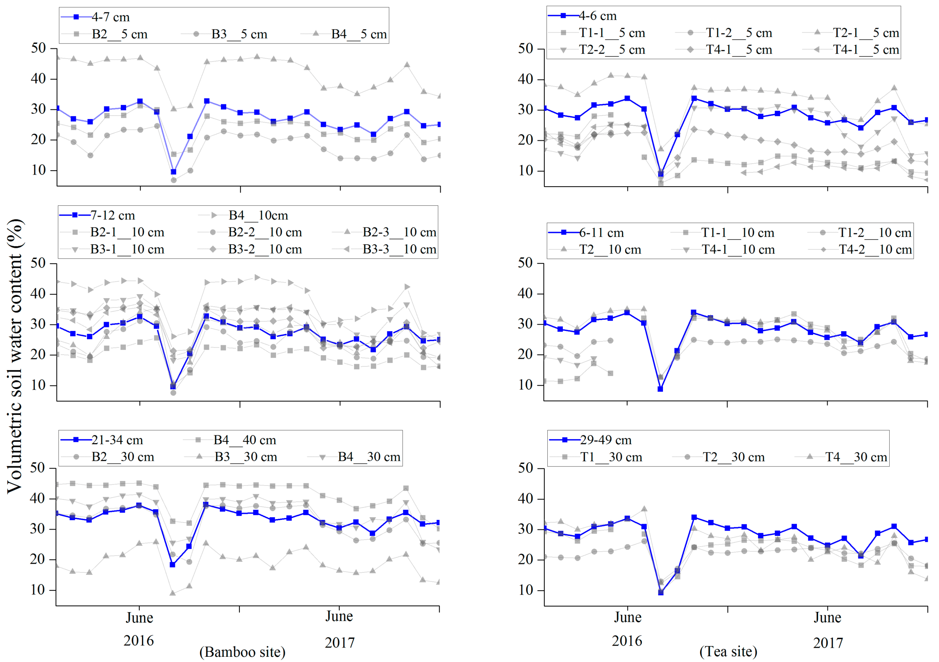
3.1. Observed and Modeled Soil Water Content

The model reproduced the seasonal dynamics of the observed soil water content at various time scales (hourly, daily, and monthly as shown in Table 1; Figure 5 and Figure S3). The exponent in the soil water retention curve, Clapp and Hornberger’s “B”, is a sensitive soil water content modeling parameter used in the CLM [33]. It was adjusted to improve the soil water content simulation at these two plots in the present study. To compensate for the effects of gravel on the soil water content at the two plots [34], it was adjusted to the lower boundary of the reasonable range for silt loam provided by Clapp and Hornberger [35]. The coefficients of determination (R2) between the observed and simulated hourly soil water contents at depths of 5, 10, and 30 cm from January 2015 to December 2017 were 0.58–0.61 (0.22–0.64), 0.50–0.63 (0.09–0.65), and 0.36–0.55 (0.36–0.52) at the bamboo (tea) plot, respectively. Similar R2 values were obtained at daily and monthly scales (Table 1; Figure S3). The simulated monthly soil water content was always within or near the ranges of the observations at a given depth (5, 10, 30, and 40 cm) at these two plots (Figure 5).
Both the observation and modeling results illustrated an obvious decrease in soil water content during August and September 2016, which was caused by the limited precipitation during August 2016 (monthly precipitation: 16.7 mm; Figure 3g). In comparison, the soil water content was larger in August and September 2017 because of greater precipitation in August 2017 (219 mm). The limited precipitation and low soil water content in August and September 2016 had a clear influence on the C cycle (see Section 3.4). Interestingly, the mean observed soil water contents at depths of 5, 10, and 30 cm at the bamboo (tea) plot were 27.95 (21.81)%, 28.14 (22.66)%, and 28.24 (24.33)%, indicating wetter soil in the bamboo than in the tea plot.

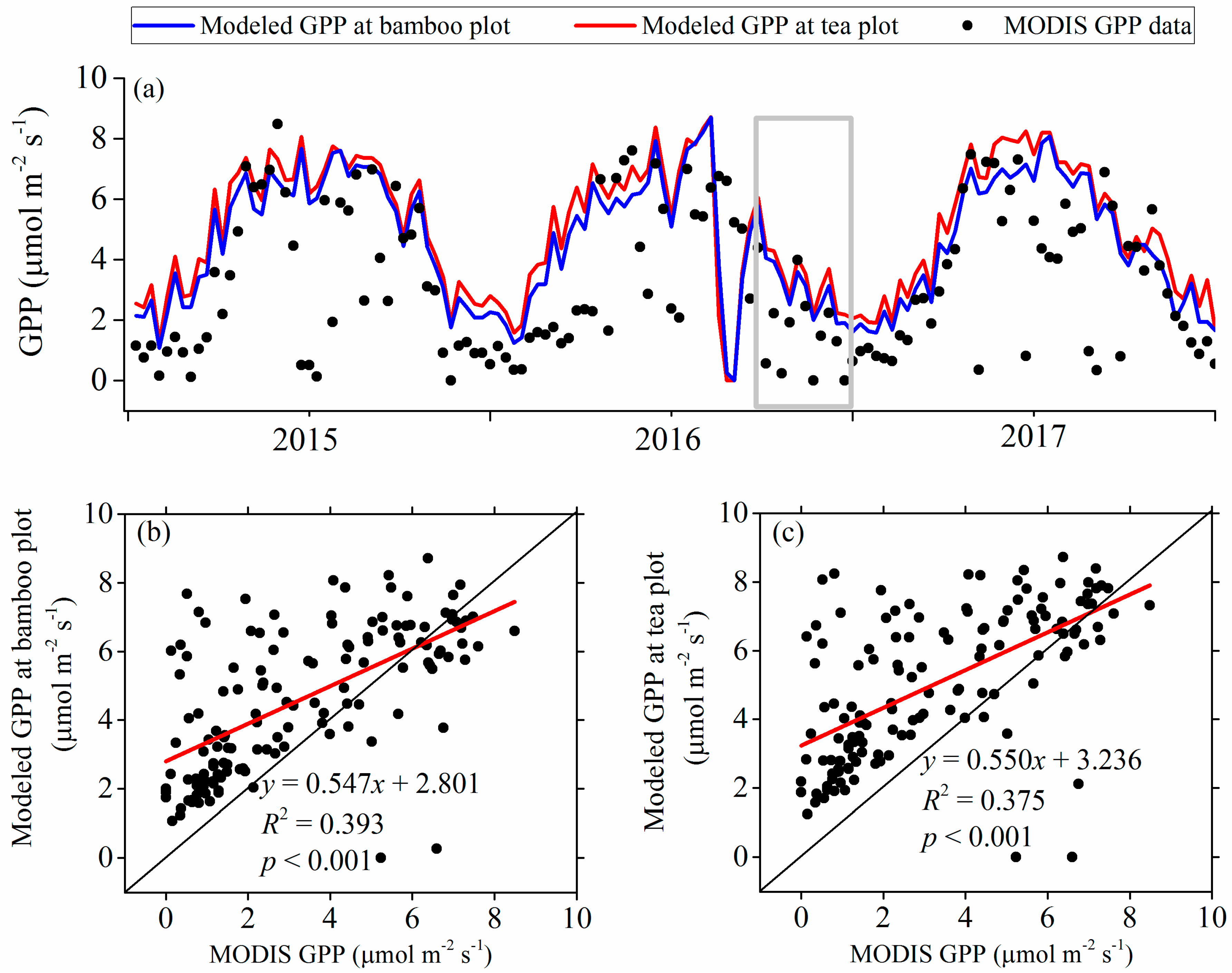
3.2. Modeled Plant Growth

The results of the model that treated bamboo as grass were not reasonable. For example, the modeled leaf area index (LAI) reached as high as 8, but decreased to 0 during the dry August of 2016 (Figure S4a), which was inconsistent with observations at the study site. Therefore, the following modeling results were obtained by considering bamboo as temperate broadleaf evergreen forest.
The modeled mean LAI values of the bamboo and tea plots during 2015–2017 were 3.3 and 4.5 (Figure S5), respectively. In comparison, the observed LAI for moso bamboo in a subtropical forest (Anji County, northwestern Zhejiang Province, China; 30°28′ N, 119°40′ E) located 115 km from the present study site was 3.6 in 2015 [36], similar to the modeled result (3.3) in the present study. The slight decrease in the observed LAI in autumn and winter and increase in spring at the Anji site were also reproduced by the model (Figure S4b). Green tea typically has a very large LAI. For example, Dutta [37] observed 36 LAI values for the same type of tea as that examined in the present study in India (Figure 1 in [37]), of which 5 values were within 3.0–4.0 and 30 within 4.0–6.5. High LAI values were observed in the photograph of our study plot (Figure 2b). Therefore, the modeled mean LAI of 4.5 for the tea plot was within a reasonable range.
The modeled GPP at the two plots was basically consistent with the MODIS GPP product (Figure 6), with the correlation R2 between simulation and MODIS GPP product being 0.39 and 0.38 at the Bamboo and tea plots, respectively. The moderate R2 (0.38–0.39) was caused the noise (e.g., close to zero GPP values during the growing season) in the MODIS product (Figure 6). The picking of the youngest leaves at the tea plot was not considered in the modeling, which could affect the carbon cycle and might contribute to the differences in GPP between modeling results and MODIS product. Both the noise in the MODIS GPP product and the neglect of the youngest leave picking in the modeling contributed to the larger modeled GPP than the MODIS value.
The modeled C storage in biomass and soil at the tea plot in the present study were consistent with previous studies, supporting the model’s accuracy. Li et al. [36] reported that the average densities of C storage in biomass, litter layer, and soil at tea plantations in China were 50.90, 4.91, and 137.50 Mg C ha−1, respectively, and no significant differences were found in the density of biomass C among different tea plant varieties and climate conditions. In the present study, the mean biomass C density, including leaf C, fine root C, coarse root C, and stem C, during 2015–2017 was 37.70 Mg C ha−1, equivalent to 74% of the value reported by Li et al. [36]. In addition, soil C accounted for the largest proportion of C storage (123.25 Mg C ha−1) during 2015–2017 in the present study, equivalent to 90% of the value reported by Li et al. [36].

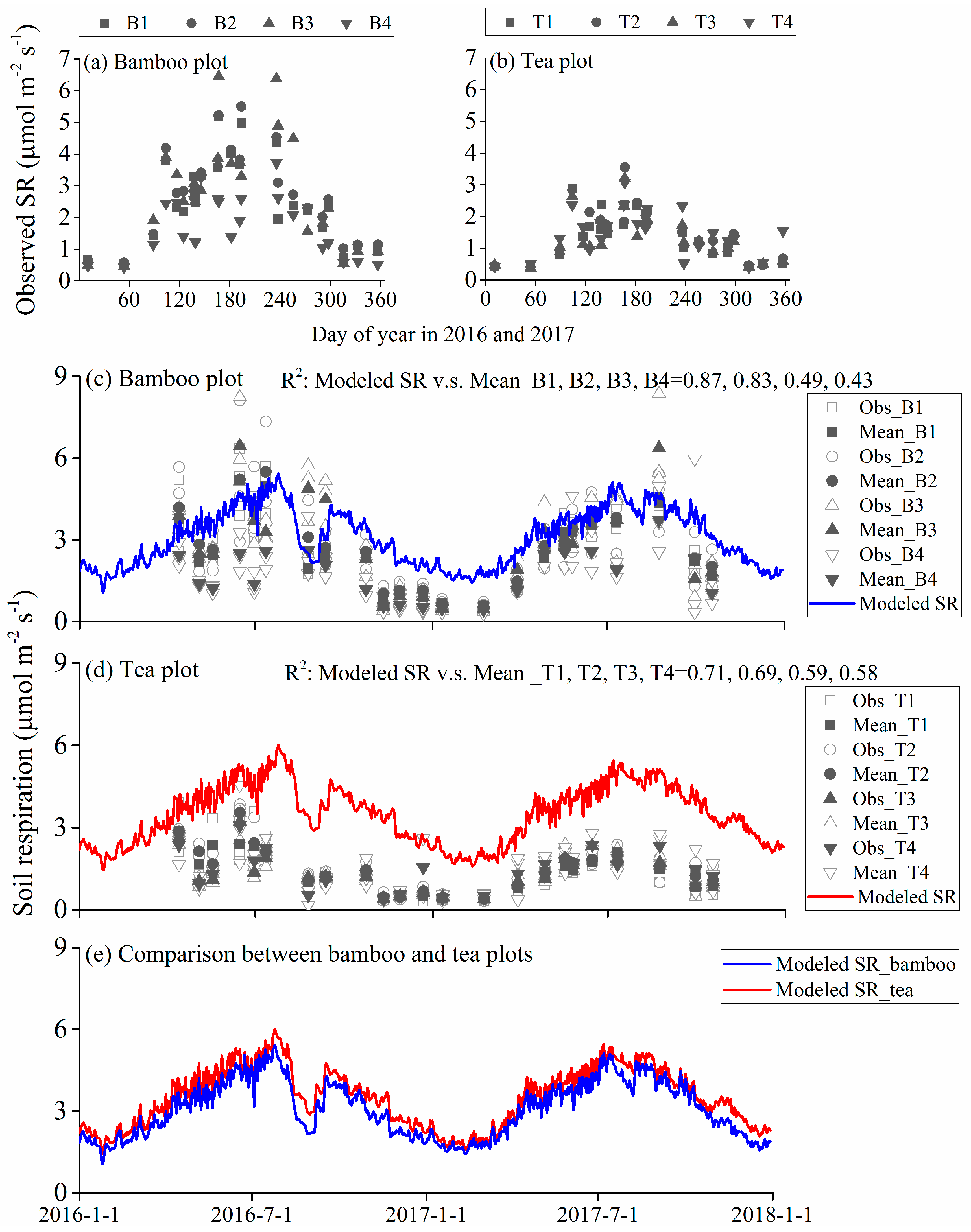
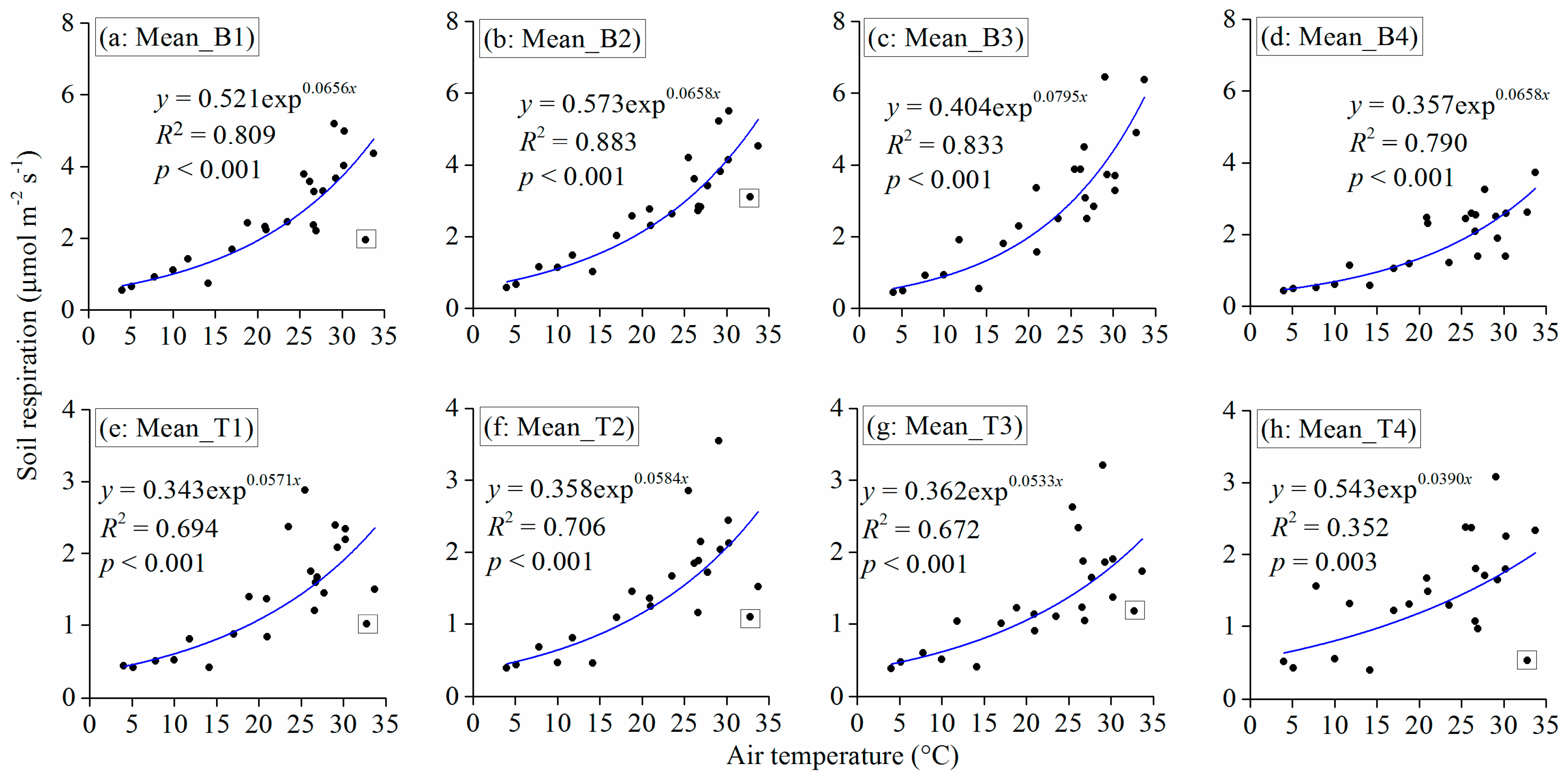
3.3. Observed and Modeled Total Soil Respiration and Heterotrophic Respiration

Figure 7 presents the measured SR data at the two plots (n = 552). At the bamboo plot, the mean (SD) observed SR values at sites B1–B4 from April 2016 to October 2017 were 2.57 (1.37), 2.79 (1.40), 2.86 (1.71), and 1.79 (0.96) µmol m−2 s−1, respectively. The modeled mean SR during 09:00–11:00 on the days when the measurements were conducted was 3.40 (0.98) µmol m−2 s−1, which was similar to the observations at sites B2 (difference: 22%) and B3 (difference: 19%). The mean hourly modeled SR during 2016–2017 was 3.14 µmol m−2 s−1, illustrating that the mean value during 09:00–11:00 (3.40) was similar to the daily value. The model also captured the seasonal dynamics of the observed SR, and the R2 values between the observed and modeled SR at sites B1–B4 were 0.87, 0.83, 0.49, and 0.43, respectively.
At the tea plot, the mean (SD) observed SR values at sites T1–T4 from April 2016 to October 2017 were 1.39 (0.73), 1.50 (0.81), 1.34 (0.73), and 1.46 (0.72) µmol m−2 s−1, respectively. The modeled mean SR (SD) and HR (SD) during 09:00–11:00 on the days when the measurements were conducted were 3.81 (0.96) and 1.57 (0.38) µmol m−2 s−1, respectively. In contrast to the bamboo plot, the modeled HR (1.57) was closer to the observed HR (1.34–1.50) than to the modeled SR (3.81). This was unsurprising, because bamboo has a fibrous root system, and the measured SR at the bamboo plot reflected the sum of RR and HR, whereas tea has a tap root system, and the measured SR between two rows at the tea plot (Figure 2b) reflected mainly HR (Figure 7d). The R2 values between the observed and modeled SR (HR) at sites T1–T4 were 0.71 (0.31), 0.69 (0.35), 0.59 (0.23), and 0.58 (0.44), respectively (Figure 7d and Figure 8b), and the correlation between the observed SR and modeled SR (Figure 7d) was markedly greater than that between the observed SR and modeled HR (Figure 8b) at all four sites, implying that RR contributed to the observed SR to some extent, although HR was the primary component of the observed SR at the tea plot.
The drought in August 2016 (monthly precipitation: 16.7 mm) caused a 55% decrease in the mean observed SR at the tea plot, from 2.12 (1.58–2.70) µmol m−2 s−1 on 12 July 2016 to 0.96 (0.17–1.32) µmol m−2 s−1 on August 25, 2016 (Figure 7d). In contrast, the corresponding mean observed SR at the bamboo plot only decreased by 23% (Figure 7c). The larger decrease in the observed SR at the tea plot (55%) than at the bamboo plot (23%) partially reflected the larger contribution of HR to the observed SR at the tea plot, because HR is influenced by soil water content and subsequent anaerobic conditions.
The simulations offered interesting results for the comparisons of SR, RR, and HR between the two plots (Figure 7e and Figure 8c). The modeled HR was larger at the bamboo plot than at the tea plot (Figure 8c), whereas the modeled SR showed the opposite trend (Figure 7e), indicative of a smaller modeled RR (SR − HR) at the bamboo plot than at the tea plot. The larger HR and smaller RR at the bamboo plot were reasonable, considering that soil water content, which influences HR, was greater at the bamboo plot than at the tea plot (Figure 5; Section 3.1), and that the LAI was larger at the tea plot (4.5) than at the bamboo plot (3.3) [38].
Both the observations and simulation showed greater SR during April–October and lower SR during November–March, consistent with the seasonal dynamics of air temperature (Figure 3, Figure 7a and Figure 9; Figure S10). Similarly, Kutsch et al. [39] reported that the rhizomicrobial respiration rate was strongly temperature dependent. In the present study, a strong exponential correlation was found between observed air temperature and soil respiration (Figure 9), which is also consistent with the monitoring results in Kutsch et al. [39] (Figure 6 in their paper). It is worth mentioning that the exponential correlation between soil respiration and temperature was decreased by the extremely dry events, as shown by the dots in small rectangles in Figure 9.

3.4. Influences of Climate and Land Use on the Carbon Cycle

The substantial differences in annual precipitation between 2015–2017 and drought in August 2016 provided a valuable opportunity to analyze the influences of climate and extremely dry events on the C cycle. The annual precipitation amounts were 1720 and 2251 mm in 2015 and 2016, respectively, and the precipitation in 2017 was 1349 mm. Therefore, 2015 and 2016 were considered to be wet and extremely wet years, respectively, while 2017 was near-normal conditions, considering the multi-year average precipitation of 1157 mm.
The modeled annual mean GPP values at the bamboo (tea) plot were 4.80 (5.21), 4.33 (4.71), and 4.57 (5.07) µmol m−2 s−1 in 2015, 2016, and 2017, respectively (Figure 10 and Figure S6). The plentiful rainfall in 2016 (2251 mm) did not increase the GPP compared with 2015 (1720 mm) and 2017 (1349 mm). This may have been due to sufficient water during normal years for plant growth in the study area; therefore, additional water does not substantially stimulate plant growth.
The modeled GPP values at the bamboo (tea) plot were 6.18 (6.48), 3.91 (3.92), and 5.31 (5.65) µmol m−2 s−1 between August–October in 2015, 2016, and 2017, respectively (Figure 10 and Figure S6), indicating that the extremely dry August in 2016 reduced the GPP during August–October, despite high precipitation in September and October in 2016 (717 mm) (Figure 10a). The MODIS GPP product also illustrated the reducing impact of drought on the GPP during August–October (shown in the grey rectangle in Figure 7a). Overall, the results indicated that the modeled GPP was not sensitive to extremely wet weather conditions but was sensitive to short periods (August 2016) of extremely dry weather conditions.
The drought in August 2016 caused marked decreases in GPP in August and the following two months (Figure 10a), while the modeled LAI was less affected (Figure S5), consistent with observations from other studies. For example, Vicca et al. [40] reported that extreme drought in Hesse, France, caused a three-year reduction in GPP in a beech forest, even though the state of the forest remained unaltered (i.e., no browning or defoliation occurred).
The monthly NEE with an absolute value greater than 0.50 µmol m−2 s−1 was defined as CO2 emissions or absorption in this study. CO2 absorption mainly occurred within (2015) or around (2016 and 2017) spring (March–May), and CO2 emissions mainly occurred in autumn (September–November) and winter (December–February). The tea plot acted as a strong CO2 emission source during the drought in August 2016 and in the following two months (Figure 10e). Both plots acted as CO2 sinks (negative NEE) in 2015 and 2017, with a mean annual NEE of −0.06 (−0.15) and −0.13 (−0.26) µmol m−2 s−1 at the Bamboo (tea) plot, respectively. In contrast, both plots acted as a CO2 source (positive NEE) in 2016, with a mean annual NEE of 0.18 and 0.29 µmol m−2 s−1, respectively. The increase in C emissions into the atmosphere after the extreme drought in 2016 (positive NEE; Figure 10e) from the modeling results was consistent with the existing understanding that extreme droughts reduce terrestrial C sinks [41].
The modeled GPP was slightly larger at the tea plot than at the bamboo plot in all months except August 2016, when the tea plot showed a slightly smaller GPP (Figure 10a). Autotrophic respiration (AR; Figure 10b) and ecosystem respiration (=AR + HR; Figure 10d) were always greater at the tea plot than the bamboo plot. The tea plot acted as a much stronger CO2 sink in 2015 and a much stronger CO2 source in 2016 compared with the bamboo plot. Temperate evergreen needle forest and mixed forest account for 20.8% and 11.7% of the total forest area in Taihu Basin. In this study, we simulated bamboo as temperate evergreen broadleaf forest. Considering the larger C sink/source of tea than bamboo during different periods, the tea ecosystem should also be a greater C sink/source than temperate evergreen needle forest in Taihu Basin.
Bamboo has a high CO2 sequestration capacity due to its rapid growth and corresponding high biomass accumulation during its early growth stage (e.g., first year); therefore, it has high potential as a woody forest for C farming and trading [16,17]. The rapid growth and high CO2 sequestration capacity of bamboo during its early growth stage are attributed to its deep and laterally extensive root system. The bamboo ecosystem in the present study was more than 20 years old and past the rapid growth stage (Figure 2a). The mean value and seasonal dynamics of the observed SR (RR + HR) were captured by the model, which implied that (a) the model effectively reproduced the C cycle of old-growth bamboo in the study, and (b) old-growth bamboo does not have as high a CO2 sequestration capacity as bamboo in the early-growth stage. Moreover, bamboo plots could act as stronger C sinks if older bamboo were harvested regularly and replaced with new growth, which did not occur at the research site during the study period. The greater observed soil water content at the bamboo plot than at the tea plot supported the low C sequestration capacity, because the soil would have been drier at the bamboo plot than at the tea plot if growth, evapotranspiration, and biomass accumulation were greater at the bamboo plot than at the tea plot.

4. Conclusions

In this study, we measured meteorological indexes, soil water content, and SR between 2016–2017 at a bamboo and green tea plot on a hillslope in the MLRYR, China. Then, we constructed mathematical models based on CLM4.5 to describe the water and C cycles for these two plots. The mean observed SR was 1.79–2.57 µmol m−2 s−1 at four bamboo sites and 1.34–1.50 µmol m−2 s−1 at four tea sites from April 2016 to October 2017. The observations illustrated the seasonal dynamics of SR, showing a peak in April–October at the two plots. The observed SR at the bamboo plot reflected both RR and HR, while the observed SR at the tea plot reflected mainly HR. Based on the good fit of the observed soil water contents at different depths at the two plots, the model effectively reproduced the seasonal dynamics of SR at the bamboo plot and HR at the tea plot. The R2 values between the observed and modeled SR were 0.43–0.87 and 0.58–0.71 for the bamboo and tea sites, respectively. The observed SR decreased by 23% and 55% due to an extreme drought in August 2016 at the bamboo and tea plots, respectively, and the model also reproduced this decrease. The modeling results indicated that tea acted as a greater C sink during spring and a greater C source during autumn and winter compared with bamboo. GPP, NPP, and NEE were affected much more by extremely dry weather than by extremely wet weather at both the bamboo and tea plots. The extremely dry period likely caused the change in both plots from a C sink to a C source and had greater influences on the tea plot.

Supplementary Materials

The following are available online at https://www.mdpi.com/1999-4907/9/10/629/s1, Figure S1: Data availability for the modeling study. FSDS, incident solar radiation; FLDS, incident longwave radiation; Temp, surface air temperature, Figure S2: Accelerated decomposition spinup and final spinup results for bamboo and tea plots, Figure S3: Observed and modeled daily soil water content at different depths at bamboo and tea plots, Figure S4: Observed (dots) and modeled (lines) leaf area index for Moso bamboo, Figure S5: Modeled leaf area index and various carbon pools, Figure S6: Modeled weekly carbon fluxes at the two study plots. AR, autotrophic respiration; ER, ecosystem respiration; GPP, gross primary production; NEE, net ecosystem exchange; NPP, net primary production.

Author Contributions

Conceptualization, C.F. and Q.Z.; Methodology, C.F., Q.Z. and Z.W.; Validation, C.F. and Q.Z.; Data Curation, Q.X. and W.X.; Writing-Original Draft Preparation, C.F.; Writing-Review & Editing, Q.Z.; Supervision, G.Y.

Funding

This study was funded by the National Natural Science Foundation of China, grant number (41622102), Pioneer Hundred Talent Program, Chinese Academy of Sciences, grant number (Y7BR021001), NIGLAS startup project for introducing talents, grant number (Y7SL041001), and Key Research Plans of Frontier Sciences, Chinese Academy of Sciences, grant number (QYZDB-SSW-DQC038).

Acknowledgments

Data for driving and validating the model are hosted at https://drive.google.com/drive/folders/1SplKoGZKdUQFYwBH8AJ368CXrVMNcxex.

Conflicts of Interest

The authors declare no conflict of interest.

References

  1. Li, M.; Feng, T.; Cai, J.; Zhou, G. Report on the World Tea Industry Development; Social Sciences Academic Press: Beijing, China, 2017; pp. 1–383. ISBN 978-7-5201-0325-1. [Google Scholar]
  2. Food and Agriculture Organization of the United Nations. World Tea Production and Trade: Current and Future Development; Food and Agriculture Organization of the United Nations: Rome, Italy, 2015. [Google Scholar]
  3. Lu, E.; Liu, S.; Luo, Y.; Zhao, W.; Li, H.; Chen, H.; Zeng, Y.; Liu, P.; Wang, X.; Higgins, R.W.; et al. The atmospheric anomalies associated with the drought over the Yangtze River basin during spring 2011. J. Geophys. Res. Atmos. 2014, 119, 5881–5894. [Google Scholar] [CrossRef] [Green Version]
  4. China Meteorological Administration (CMA). China Climate Bulletin; CMA: Beijing, China, 2016. [Google Scholar]
  5. Herring, S.; Christidis, N.; Hoell, A.; Kossin, J.; Schreck, I.I.I.C.; Stott, P. Explaining Extreme Events of 2016 from a Climate Perspective. Bull. Am. Meteorol. Soc. 2018, 99, S1–S157. [Google Scholar] [CrossRef] [Green Version]
  6. Allan, R.; Soden, B. Atmospheric warming and amplification of precipitation extremes. Science 2008, 321, 1481–1484. [Google Scholar] [CrossRef] [PubMed]
  7. Utsumi, N.; Seto, S.; Kanae, S.; Maeda, E.E.; Oki, T. Does higher surface temperature intensify extreme precipitation? Geophys. Res. Lett. 2011, 38, L16708. [Google Scholar] [CrossRef]
  8. Fischer, E.M.; Kutti, R. Observed heavy precipitation increase confirms theory and early models. Nat. Clim. Chang. 2016, 6, 986–991. [Google Scholar] [CrossRef]
  9. Wang, G.; Wang, D.; Trenberth, K.E.; Erfanian, A.; Yu, M.; Bosilovich, M.G.; Parr, D.T. The peak structure and future changes of the relationships between extreme precipitation and temperature. Nat. Clim. Chang. 2017, 7, 268–275. [Google Scholar] [CrossRef]
  10. Sterl, A.; Severijns, C.; Dijkstra, H.; Hazeleger, W.; van Oldenborgh, G.J.; van den Broeke, M.; Burgers, G.; van den Hurk, B.; van Leeuwen, P.J.; van Velthoven, P. When can we expect extremely high surface temperatures? Geophys. Res. Lett. 2008, 35, L14703. [Google Scholar] [CrossRef]
  11. Allen, C.D.; Macalady, A.K.; Chenchouni, H.; Bachelet, D.; Mcdowell, N.; Vennetier, M.; Kitzberger, T.; Rigling, A.; Breshears, D.D.; Hogg, E.H.; et al. A global overview of drought and heat-induced tree mortality reveals emerging climate change risks for forests. For. Ecol. Manag. 2010, 259, 660–684. [Google Scholar] [CrossRef]
  12. IPCC. Climate Change 2013: The Physical Science Basis. Contribution of Working Group I to the Fifth Assessment Report of the Intergovernmental Panel on Climate Change; Stocker, T.F., Qin, D., Plattner, G.K., Tignor, M., Allen, S.K., Boschung, J., Nauels, A., Xia, Y., Bex, V., Midgley, P.M., Eds.; Cambridge University Press: Cambridge, UK; New York, NY, USA, 2013; 1535p. [Google Scholar] [CrossRef]
  13. Zhang, Q.; Li, Q.; Singh, V.P.; Shi, P.; Huang, Q.; Sun, P. Nonparametric integrated agrometeorological drought monitoring: Model development and application. J. Geophys. Res. Atmos. 2018, 123, 73–88. [Google Scholar] [CrossRef]
  14. Yang, J.; Li, M.; Xiao, L.; Zhou, H.; Guan, X.; Li, X.; Su, Z.; Xie, X.; Zong, Q.; Yang, Q. Annual Reports on China’s Tea Industry; Social Sciences Academic Press: Beijing, China, 2017; ISBN 978-7-5201-1707-4. [Google Scholar]
  15. SFAPRC. Forest Resources in China—The 8th National Forest Inventory; State Forestry Administration: Beijing, China, 2015. [Google Scholar]
  16. Song, X.; Zhou, G.; Jiang, H.; Yu, S.; Fu, J.; Li, W.; Wang, W.; Ma, Z.; Peng, C. Carbon sequestration by Chinese bamboo forests, and their ecological benefits: Assessment of potential, problems, and future challenges. Environ. Rev. 2011, 19, 418–428. [Google Scholar] [CrossRef]
  17. Nath, A.J.; Lal, R.; Das, A.K. Managing woody bamboos for carbon farming and carbon trading. Glob. Ecol. Conserv. 2015, 3, 654–663. [Google Scholar] [CrossRef]
  18. McClure, F.A. The Bamboos: A Fresh Perspective; Harvard University Press: Cambridge, MA, USA, 1966; p. 345. [Google Scholar]
  19. Xu, X.; Yang, G.; Tan, Y.; Tang, X.; Jiang, H.; Sun, X.; Zhuang, Q.; Li, H. Impacts of land use changes on net ecosystem production in the Taihu Lake Basin of China from 1985 to 2010. J. Geophys. Res. Biogeosci. 2017, 122, 690–707. [Google Scholar] [CrossRef]
  20. Liao, K.; Lv, L.; Yang, G.; Zhu, Q. Sensitivity of simulated hillslope subsurface flow to rainfall patterns, soil texture and land use. Soil Use Manag. 2016, 32, 422–432. [Google Scholar] [CrossRef]
  21. Liao, K.; Zhou, Z.; Lai, X.; Zhu, Q.; Feng, H. Evaluation of different approaches for identifying optimal sites to predict mean hillslope soil moisture content. J. Hydrol. 2017, 547, 10–20. [Google Scholar] [CrossRef]
  22. Lai, X.; Zhou, Z.; Zhu, Q.; Liao, K. Comparing the spatio-temporal variations of soil water content and soil free water content at the hillslope scale. Catena 2018, 160, 366–375. [Google Scholar] [CrossRef]
  23. Lai, X.; Zhu, Q.; Zhou, Z.; Liao, K. Influences of sampling size and pattern on the uncertainty of correlation estimation between soil water content and its influencing factors. J. Hydrol. 2017, 555, 41–50. [Google Scholar] [CrossRef]
  24. Hutchinson, G.L.; Livingston, G.P. Use of chamber systems to measure trace gas fluxes. In Agricultural Ecosystem Effects on Trace Gases and Global Climate; Harper, L.A., Ed.; American Society of Agronomy: Madison, WI, USA, 1993; pp. 79–93. [Google Scholar]
  25. Oleson, K.; Lawrence, D.M.; Bonan, G.B.; Drewniak, B.; Huang, M.; Koven, C.D.; Levis, S.; Li, F.; Riley, W.J.; Subin, Z.M.; et al. Technical Description of Version 4.5 of the Community Land Model (CLM); NCAR Technical Note NCAR/TN-503CSTR; NCAR: Boulder, CO, USA, 2013; 420p. [Google Scholar]
  26. Running, S.W.; Hunt, E.R., Jr. Generalization of a forest ecosystem process model for other biomes, BIOME-BGC, and an applicationfor global-scale models. In Scaling Physiological Processes: Leaf to Globe; Ehleringer, J.R., Field, C., Eds.; Academic Press: San Diego, CA, USA, 1993; pp. 141–158. [Google Scholar]
  27. White, M.A.; Thornton, P.E.; Running, S.W.; Nemani, R.R. Parameterization and sensitivity analysis of the Biome-BGC terrestrial ecosystem model: Net primary production controls. Earth Interact. 2000, 4, 1–85. [Google Scholar] [CrossRef]
  28. Thornton, P.E.; Law, B.E.; Gholz, H.L.; Clark, K.L.; Falge, E.; Ellsworth, D.S.; Goldstein, A.H.; Monson, R.K.; Hollinger, D.; Falk, M.; et al. Modeling and measuring the effects of disturbance history and climate on carbon and water budgets in evergreen needleleaf forests. Agric. For. Meteorol. 2002, 113, 185–222. [Google Scholar] [CrossRef]
  29. Parton, W.; Stewart, J.; Cole, C. Dynamics of C, N, P and S in Grassland Soils—A Model. Biogeochemistry 1988, 5, 109–131. [Google Scholar] [CrossRef]
  30. Fu, C.; Lee, X.; Griffis, T.J.; Wang, G.; Wei, Z. Influences of root hydraulic redistribution on N2O emissions at AmeriFlux sites. Geophys. Res. Lett. 2018, 45, 5135–5143. [Google Scholar] [CrossRef]
  31. Fu, C.; Wang, G.; Bible, K.; Goulden, M.L.; Saleska, S.R.; Scott, R.L.; Cardon, Z.G. Hydraulic redistribution affects modeled carbon cycling via soil microbial activity and suppressed fire. Glob. Chang. Biol. 2018, 24, 3472–3485. [Google Scholar] [CrossRef] [PubMed]
  32. Thornton, P.E.; Rosenbloom, N.A. Ecosystem model spin-up: Estimating steady state conditions in a coupled terrestrial carbon and nitrogen cycle model. Ecol. Model. 2005, 189, 25–48. [Google Scholar] [CrossRef]
  33. Fu, C.; Wang, G.; Goulden, M.L.; Scott, R.L.; Bible, K.; Cardon, Z.G. Combined measurement and modeling of the hydrological impact of hydraulic redistribution using CLM4.5 at eight AmeriFlux sites. Hydrol. Earth Syst. Sci. 2016, 20, 2001–2018. [Google Scholar] [CrossRef]
  34. Zhu, Q.; Castellano, M.J.; Yang, G.S. Coupling soil water processes and nitrogen cycle across spatial scales: Potentials, bottlenecks and solutions. Earth-Sci. Rev. 2018. [Google Scholar] [CrossRef]
  35. Clapp, R.B.; Hornberger, G.M. Empirical equations for some soil hydraulic properties. Water Resour. Res. 1978, 14, 601–604. [Google Scholar] [CrossRef]
  36. Li, X.; Mao, F.; Du, H.; Zhou, G.; Xu, X.; Han, N.; Sun, S.; Gao, G.; Chen, L. Assimilating leaf area index of three typical types of subtropical forest in China from MODIS time series data based on the integrated ensemble Kalman filter and PROSAIL model. ISPRS J. Photogramm. Remote Sens. 2017, 126, 68–78. [Google Scholar] [CrossRef]
  37. Dutta, R. Impact of age and management factors on tea yield and modelling the influence of leaf area index on yield variations. Sci. Asia 2011, 37, 83–87. [Google Scholar] [CrossRef]
  38. Wei, Z.; Yoshimura, K.; Wang, L.; Miralles, D.; Jasechko, S.; Lee, X. Revisiting the contribution of transpiration to global terrestrial evapotranspiration. Geophys. Res. Lett. 2017, 44, 2792–2801. [Google Scholar] [CrossRef]
  39. Kutsch, W.L.; Staack, A.; Wötzel, J.; Middelhoff, U.; Kappen, L. Field measurements of root respiration and total soil respiration in an alder forest. New Phytol. 2001, 150, 157–168. [Google Scholar] [CrossRef] [Green Version]
  40. Vicca, S.; Balzarolo, M.; Filella, I.; Granier, A.; Herbst, M.; Knohl, A.; Longdoz, B.; Mund, M.; Nagy, Z.; Pintér, K.; et al. Remotely-sensed detection of effects of extreme droughts on gross primary production. Sci. Rep. 2016, 6, 28269. [Google Scholar] [CrossRef] [PubMed] [Green Version]
  41. Reichstein, M.; Bahn, M.; Ciais, P.; Frank, D.; Mahecha, M.D.; Seneviratne, S.I.; Zscheischler, J.; Beer, C.; Buchmann, N.; Frank, D.C.; et al. Climate extremes and the carbon cycle. Nature 2013, 500, 287–295. [Google Scholar] [CrossRef] [PubMed]
Figure 1. Location of the study site and distribution of the sampling points for soil moisture and soil respiration.
Forests 09 00629 g001
Figure 2. Images of the (a) moso bamboo and (b) green tea plots, and (c) image and (d) diagram of the soil respiration monitoring instrument.
Forests 09 00629 g002
Figure 3. Meteorological data used to drive the model. (a) FSDS, incident solar radiation; (b) FLDS, incident longwave radiation; (c) PBOT, atmospheric pressure; (d) air temperature; (e) wind speed, and (f) precipitation.
Forests 09 00629 g003
Figure 4. Schematic of the method used in the study. FSDS, P, T, RH, and Wind represent incoming solar radiation, rainfall, air temperature, relative humidity, and wind speed, respectively.
Forests 09 00629 g004
Figure 5. Observed and modeled soil water content by soil depth at the two study plots.
Forests 09 00629 g005
Figure 6. MODIS and the modeled 8-day Gross Primary Production (GPP) at the study site. The grey rectangle shows the period when drought affects GPP. (a) time series of the modeled GPP and MODIS data; correlations between MODIS and the modeled GPP at bamboo (b) and tea (c) plot.
Forests 09 00629 g006
Figure 7. Observed and modeled soil respiration (SR) at the two study plots. (a,b) show the seasonal dynamics of the observed SR at the bamboo and tea plots, respectively; (ce) show the time series of the observed and modeled SR.
Forests 09 00629 g007
Figure 8. Observed soil respiration (SR) and modeled heterotrophic respiration (HR) at the bamboo (a) and tea (b) plots. Panel (c) shows the comparisons between the modeled HR at the two plots.
Forests 09 00629 g008
Figure 9. Correlations between observed air temperature and soil respiration at bamboo (panels (ad): sites B1–B4) and tea (panels (eh): sites T1–T4) plots. Both air temperature and soil respiration were observed between 9:00–11:00 Dots in squares were soil respirations that were observed during the dry August of 2016.
Forests 09 00629 g009
Figure 10. Modeled monthly carbon fluxes at the two study plots. (a) AR, autotrophic respiration; (b) ER, ecosystem respiration; (c) GPP, gross primary production; (d) NEE, net ecosystem exchange; (e) NPP, net primary production.
Forests 09 00629 g010
Table 1. Hourly (daily, monthly) R2 between observed and simulated soil water content.
Bamboo Plot 4–7 cm7–12 cm21–34 cm
B15 cm0.58 (0.61, 0.65)
10 cm_10.56 (0.63, 0.65)
10 cm_20.53 (0.57, 0.70)
10 cm_30.56 (0.58, 0.54)
30 cm0.36 (0.40, 0.49)
B25 cm0.61 (0.64, 0.62)
10 cm_10.63 (0.64, 0.60)
10 cm_20.53 (0.54, 0.47)
10 cm_30.54 (0.60, 0.49)
30 cm0.55 (0.52, 0.53)
B45 cm0.59 (0.61, 0.62)
10 cm0.50 (0.55, 0.50)
30 cm0.51 (0.52, 0.51)
40 cm0.47 (0.48, 0.47)
Tea Plot 4–6 cm6–11 cm29–49 cm
T25 cm_10.22 (0.21, 0.32)
5 cm_20.64 (0.64, 0.41)
10 cm_10.09 (0.09, −)
10 cm_20.43 (0.44, 0.28)
30 cm0.52 (0.54, 0.74)
T35 cm_10.60 (0.63, 0.74)
5 cm_20.24 (0.23, 0.22)
10 cm0.60 (0.65, 0.72)
30 cm0.36 (0.44, 0.55)
T45 cm_10.62 (0.67, 0.75)
5 cm_20.39 (0.39, 0.42)
10 cm_10.65 (0.68, 0.80)
10 cm_20.40 (0.41, −)
30 cm0.47 (0.55, 0.61)

