Estimating Forest Canopy Cover in Black Locust (Robinia pseudoacacia L.) Plantations on the Loess Plateau Using Random Forest

Abstract

The forest canopy is the medium for energy and mass exchange between forest ecosystems and the atmosphere. Remote sensing techniques are more efficient and appropriate for estimating forest canopy cover (CC) than traditional methods, especially at large scales. In this study, we evaluated the CC of black locust plantations on the Loess Plateau using random forest (RF) regression models. The models were established using the relationships between digital hemispherical photograph (DHP) field data and variables that were calculated from satellite images. Three types of variables were calculated from the satellite data: spectral variables calculated from a multispectral image, textural variables calculated from a panchromatic image (T_pan) with a 15 × 15 window size, and textural variables calculated from spectral variables (T_B+VIs) with a 9 × 9 window size. We compared different mtry and ntree values to find the most suitable parameters for the RF models. The results indicated that the RF model of spectral variables explained 57% (root mean square error (RMSE) = 0.06) of the variability in the field CC data. The soil-adjusted vegetation index (SAVI) and enhanced vegetation index (EVI) were more important than other spectral variables. The RF model of T_pan obtained higher accuracy (R² = 0.69, RMSE = 0.05) than the spectral variables, and the grey level co-occurrence matrix-based texture measure—Correlation (COR) was the most important variable for T_pan. The most accurate model was obtained from the T_B+VIs (R² = 0.79, RMSE = 0.05), which combined spectral and textural information, thus providing a significant improvement in estimating CC. This model provided an effective approach for detecting the CC of black locust plantations on the Loess Plateau.

1. Introduction

Forest canopy cover (CC), which is defined as the proportion of the forest floor that is covered by the vertical projection of the tree crown [1], plays a major role in understanding the structure and health condition of forest ecosystems [2]. It is also a useful measure for evaluating the leaf area index (LAI), carbon stocks, tree density, and wildlife microhabitat [3,4,5,6]. The growth and diversity of understory vegetation is also related to CC [7]. In addition, the forest CC and understory vegetation play an important role in minimize the rate of soil loss by reducing the erosive effects of rainfall with interception [8]. The Loess Plateau of China has experienced severe soil erosion, vegetation degradation, and desertification [9]. Black locust (Robinia pseudoacacia L.) represents the most abundant type of plantation on the Loess Plateau, and these plantations provide a wide range of ecological and socio-economic functions [10,11]. Accurate and regular measurements of the CC of black locust plantations are important and can be used to monitor forest degradation and desertification on the Loess Plateau [12].

There are two common approaches for CC estimation: field measurements and remote sensing. Field-based methods are the most accurate estimation approaches. Optical instruments, such as digital hemispherical photographs (DHPs), LAI-2200 plant canopy analyzers, and AccuPAR Ceptometers are widely adopted for CC acquisition due to their non-destructive nature [13]. However, these methods suffer from many shortcomings; for example, they are time-consuming, labor-intensive, and difficult to apply for large areas [5,14]. Thus, a method is needed that can be used to easily extract forest CC over a large area. Remote sensing techniques can represent such a method, because they offer new strategies for measuring forest CC from local to global scales [3,12,15,16,17,18]. Different type of sensors such as aerial photo, satellite images and active sensors (e.g., LiDAR, SAR, and RADAR) have been applied to estimate forest CC [18,19,20]. The unmanned aerial vehicle (UAV) with high acquisition flexibility and resolution appears to be very promising for the assessment of CC, but only if the forest is widely open and a precise digital terrain model is available [21]. Ma et al. [20] compared LiDAR, aerial imagery and satellite imagery in CC estimation, and found that LiDAR-derived CC were marginally influenced by the estimation algorithms and generate comparable results. The major limitations in aerial photo were distortion and the presence of shadows. While the distortion and shadow have less impact on satellite imagery since these images were collected at high altitude [20]. The active sensors also have some limitations, such as challenging processing requirements and complex interactions with forest structure. Wallis et al. [22] noted that optical remote sensing data can be substituted for LiDAR data in habitat diversity studies. Optical sensors are still a popular choice for forest parameter estimation. In this research, we select a satellite image to estimate CC.

A range of variables is calculated from satellite images for CC estimation. Spectral vegetation indices (VIs), such as the normalized difference vegetation index (NDVI), the soil-adjusted vegetation index (SAVI), and the enhanced vegetation index (EVI), have been used to estimate CC in monospecific and mixed forests [18,19,23,24]. For example, Korhonen et al. [18] used NDVI, atmospherically resistant vegetation index (ARVI), and simple ration (SR) to estimate CC in tropical forests based on ALOS AVNIR-2 image. The NDVI, SR, and SAVI derived from SPOT 5 satellite data were used to estimate CC by Chasmer et al. [25], their results indicated that the NDVI and SAVI are more comparable to CC. In addition, González-Roglich and Swenson [5] studied the tree cover and carbon of Argentine savannas using seven VIs that are based on the China Brazil Earth Resources Satellite series and Landsat images. Karlson et al. [24] estimated the tree CC and aboveground biomass using six VIs based on the Landsat 8 OLI in a woodland landscape. However, spectral variables suffer from saturation and multiple layering problems in high canopy regions [11,26].

With recent high-resolution imagery, such as QuickBird and IKONOS, forest CC can be recognized at a crown level. When spatial resolution increases, the objects on the ground tend to be represented by few pixels; therefore, the spatial information becomes increasingly important when compared with spectral information. The texture calculated from high spatial resolution images can enhance the discrimination of spatial information and improve detection levels by increasing saturation levels [11,27,28]. Li et al. [19], Sarker and Nichol [27], and Wood et al. [29] all found that textural variables provided a larger contribution than spectral variables for forest parameter estimations. Tuanmu and Jetz [30] demonstrated that the texture measures of the EVI were superior to the conventional topography- and land-cover-based metrics in terms of their ability to capture fine-grain habitat heterogeneity and predict key biodiversity patterns across a large extent. Combining spatial detail and unique spectral information leverages complementary information, which could improve the accuracy of estimating canopy properties [11,31]. Gu et al. [16] reported that a combination of VIs and texture can improve the accuracy of estimating vegetation fractional coverage of planted and natural forests. Halperin et al. [12] used spectral and textural variables to estimate the CC in the Miombo woodlands of Zambia, and they found that the texture was more prominent in the imagery and that a combination of spectral and textural variables provided the best estimation. Pu et al. [28] demonstrated similar results that the combination of spectral and textural variables could generate higher accuracy than their either one separately in mapping forest LAI.

Many parametric and non-parametric methods have been used for predicting forest structure parameters. Parametric methods, such as traditional linear regression models, were the most widely used models in the last decades [3,11,26,28], and they are simple and easy to explain [32]. The traditional linear models have an explicit model structure and they can be specified by parameters [33]. The relationship between predictors and response variables can be explained from an ecological perspective [34]. However, these models make strong assumptions about the data, and multicollinearity problems may occur [35]. The models usually obtain moderate accuracy, and their performance mainly depends on the goodness of these assumptions [34]. In contrast, non-parametric methods have fewer assumptions, higher methodological accuracy, and high non-linear adaptation [36]. The major drawback of these models is uneasy interpreting, because it seems more of a “black box” [32,34]. The structure developed for many remote sensing regression applications can be very complex and it is impossible to derive meaningful interpretation. Even so, the non-parametric approaches are becoming more popular, especially since there a diverse array of spatially-explicit explanatory variables that are available to researchers. One of the most widely adopted approaches used for CC estimation is random forest (RF) regression models. The RF algorithm can be used to reduce input data dimension and the variable importance measurement could identify the most relevant remote sensing variables [37,38]. Pullanagari et al. [39] evaluated pasture quality using RF combined with recursive feature elimination, and obtained stable result with improved accuracy. Karlson et al. [24] used RF and Landsat 8 OLI to map the CC of trees and the aboveground biomass in the Sudano-Sahelian woodlands. In addition, the RF has been successfully applied in land use and land cover classification, this method provide higher accuracy when compared to maximum likelihood classifier, CART and SVM [38,40,41]. Shataee et al. [42] and Cracknell and Reading [43] indicated that RF was superior to other non-parametric approaches in predicting forest parameters and supervised classification for lithology. This method can easily train and stabilize a range of model parameter values [44]. The potential of RF to predict the CC of black locust plantations on the Loess Plateau has not received much attention.

The objectives of this study are to demonstrate a potential approach for modeling and mapping black locust plantations CC on the Loess Plateau using QuickBird imagery. Specifically, the goals are to (1) identify the optimal window size and suitable parameters of RF models; (2) compare the performance of three types of variables in modeling the CC of black locust plantations, i.e., spectral variables (Bands + VIs), textural variables calculated from panchromatic image (T_pan) and textural variables calculated from spectral variables (T_B+VIs); and, (3) map the CC in the black locust plantations using the most accurate RF regression model. The results obtained in this study are conducive to efficiently estimating the CC. A CC map is an effective tool for detecting the state of forest areas and the associated forest health conditions, both of which can be used in developing forest management plans on the Loess Plateau of China.

2. Materials and Methods

2.1. Study Area

The study area is located in Yongshou County of Shaanxi Province on the southern Loess Plateau of China (34°44′–34°56′ N and 107°56′–108°09′ E) (Figure 1). The region has a semi-humid, temperate continental climate with a mean temperature of 7–13.3 °C. The average annual precipitation is 601.6 mm, of which more than 53% falls between July and September. The soil type at the study site is cinnamon soil (based on the Chinese Soil Taxonomy). The study area is located in the loess hilly-gully region and it has an elevation ranging from 1060 to 1508 m above sea level. The forest is distributed across two sites, the Huaiping forest farm and the Maliantan forest farm, and it is dominated by black locust plantations (Robinia pseudoacacia L.), which account for about 90% of the forested area.

2.2. Field Data

A field survey of the sample plots was performed from 16 June to 15 July 2012. Overall, 74 plots were randomly distributed within pure black locust plantation forest areas, where the forest area was delimited by the satellite image based on the National Forest Inventory (NFI) data. Each plot was 20 × 20 m in size. The CC, diameter at breast height (DBH), tree height, crown diameter, and stand density were measured in each plot. Trees with a DBH less than 5 cm were not included. A differential global positioning system was used to determine the center and the four corners of each plot, thus allowing for the plots to be geo-referenced with satellite data. The field data characteristics are summarized in

Table 1. Summary of the characteristics of the forest field plots.

Variable (Unit)	Minimum	Maximum	Mean	Standard Deviation
CC	0.28	0.88	0.67	0.10
DBH (cm)	5.38	26.41	12.58	4.80
Crown Diameter (m)	2.02	5.81	3.51	0.88
Density (N/ha)	250	2775	1228	676
Height (m)	5.38	19.98	11.98	3.03

.

DHPs were obtained to calculate the forest CC. The DHPs were collected from five randomly selected locations in each plot using a Nikon Coolpix 4500 (Nikon Corp., Tokyo, Japan) digital camera in combination with an FC-E8 Circular Fisheye lens. The camera and lens provided a focal length equivalent of 6 mm, a combined f-stop of f/2.8, and a full 180-degree field-of-view. The camera was mounted on a tripod, leveled using a two-axis camera-mounted bubble level, oriented to magnetic north, and positioned 1.3 m above ground level. Overhead branches were avoided, and the camera exposure time was set to automatic. To avoid the effects of sunlight, we chose a time close to sunrise (or sunset) under uniform sky conditions and not during common working hours to avoid the interference of direct sunlight. All of the images were shot at “fine” quality and the maximum resolution (2048 pixels × 1536 pixels) of the camera. Images were saved in JPEG format.

Each DHP was analyzed with Gap Light Analyzer 2.0 (Simon Fraser University, Burnaby, BC, Canada) [45]. In this study, we used the blue channel and a threshold of 128 to calculate the CC of each photograph. The blue band is preferred because this portion of the spectrum is superior for separating pixels into forest canopy and sky classes [45,46,47]. Several authors have noted that subjective adjustment of the threshold can be a source of error because it is somewhat arbitrary [47,48]. To overcome these subjectivity issues, we use a constant threshold of 128 (half of a 256-bit image) to separate the sky and canopy of each photograph [49,50]. Then, the CC was calculated, as follows.

$$\mathrm{CC}=\frac{\mathrm{Total}\mathrm{pixels}-\mathrm{Sky}\mathrm{pixels}}{\mathrm{Total}\mathrm{pixels}}$$

(1)

The CC was calculated for each DHP, and the average of five photographs was calculated in each plot.

2.3. Remote Sensing Data

The QuickBird multispectral and panchromatic images used in this study were obtained on 22 June 2012, and the spatial resolution was 0.61 m for the panchromatic image and 2.44 m for the multispectral image. The multispectral image had four bands, including blue (450–520 nm), green (520–600 nm), red (630–690 nm), and near-infrared (760–900 nm) bands. The panchromatic image was ortho-rectified using the ENVI 5.1 software package (Exelis Visual Information Solutions, Boulder, CO, USA). Fifty high-quality and well-distributed ground control points (GCPs) that were obtained via the field survey using differential global positioning system equipment were used for ortho-rectification. A digital elevation model (DEM) (1:10,000) derived from stereo aerial photographs with a resolution of 5 m was also used to ortho-rectify the QuickBird panchromatic image. The overall error was 0.68 pixels. Then, the corrected panchromatic image was used to rectify the multispectral image, resulting in an overall error of 0.34 pixels. The raw digital numeric values of the multispectral image were converted to spectral radiance and subsequently to top of atmosphere (TOA) reflectance. Atmospheric correction was performed using the Fast Line-of-sight Atmospheric Analysis of Spectral Hypercubes (FLAASH) approach to remove the scattering and absorption effects from the atmosphere and to obtain the surface reflectance character. The non-black locust area was manually masked from the image based on the NFI data.

2.4. Predictor Variables

2.4.1. Spectral Variables

The spectral variables that were extracted from the QuickBird multispectral image included four reflectance bands (B1-blue, B2-green, B3-red, and B4-NIR) and eight VIs (

Table 2. Selected vegetation indices (VIs) used for canopy cover (CC) estimation [11].

Spectral Vegetation Indices
1. Simple Ratio (SR) = $\frac{\mathrm{NIR}}{\mathrm{R}}$
2. Soil Adjusted Vegetation Index (SAVI) = $(1+\mathrm{L})\frac{\mathrm{NIR}-\mathrm{R}}{\mathrm{NIR}+\mathrm{R}+\mathrm{L}}$
3. Enhanced Vegetation index (EVI) = $\mathrm{G}\frac{\mathrm{NIR}-\mathrm{R}}{{\mathrm{NIR}+\mathrm{C}}_1{\mathrm{R}-\mathrm{C}}_2\mathrm{B}+\mathrm{L}}$
4. Atmospherically Resistant Vegetation Index (ARVI) = $\frac{\mathrm{NIR}-\mathrm{RB}}{\mathrm{NIR}+\mathrm{RB}}$, RB = $\mathrm{R}-\mathsf{\gamma }(\mathrm{B}-\mathrm{R})$
5. Modified Soil Adjusted Vegetation Index (MSAVI) = $\left[\left(2\mathrm{NIR}+1\right)-\sqrt{{\left(2\mathrm{NIR}+1\right)}^2-8\left(\mathrm{NIR}-\mathrm{R}\right)}\right]/2$
6. Non-linear Vegetation index (NLI) = $\frac{{\mathrm{NIR}}^2-\mathrm{R}}{{\mathrm{NIR}}^2+\mathrm{R}}$
7. Difference Vegetation index (DVI) = $\mathrm{NIR}-\mathrm{R}$
8. Normalized Difference Vegetation Index (NDVI) = $\frac{\mathrm{NIR}-\mathrm{R}}{\mathrm{NIR}+\mathrm{R}}$

B, R, and NIR represent the QuickBird reflectance for the blue, red and near-infrared wavelengths, respectively. Parameters L and γ represent the SAVI term (set equal to 0.5) and the ARVI term (set equal to 1), respectively. The coefficients adopted in the EVI algorithm are L = 1.0, C₁ = 6.0, C₂ = 7.5, and G (gain factor) = 2.5 [51].

). The VIs combine information from two or more spectral bands to enhance the vegetation signal while minimizing soil, atmospheric, and solar irradiance effects [51]. This study analyzed the correlations between the different spectral variables and the forest CC obtained from the DHP data.

2.4.2. Textural Variables Calculated from Panchromatic Image (T_pan)

Image texture, which is defined by Haralick et al. [52] as “the pattern of spatial distributions of grey-tone”, describes the relationships among surface cover elements. The texture of an image contains valuable information about the spatial and structural arrangement of objects [26,52]. In our research, eight widely used Grey Level Co-occurrence Matrix (GLCM) measures that were proposed by Haralick et al. [52] were selected (

Table 3. Formulas for the texture measurements used in this study [52].

Grey Level Co-occurrence Matrix (GLCM) Based Texture Parameter Estimation
1. Mean (MEAN) = ${\sum }_{i,j=0}^{N-1}p\left(i,j\right)$
2. Homogeneity (HOM) = ${\sum }_i{\sum }_j\frac{p\left(i,j\right)}{1+{\left(i-j\right)}^2}$
3. Contrast (CON) = ${\sum }_{n=0}^{N-1}{n}^2\{{\sum }_{i=1}^N{\sum }_{j=1}^{N}p(i,j)\}$
4. Dissimilarity (DIS) = ${\sum }_{n=0}^{N-1}n\{{\sum }_{i=1}^N{\sum }_{j=1}^{N}p(i,j)\}$
5. Entropy (ENT) = $-{\sum }_i{\sum }_{j}p\left(i,j\right)\log \left(p\left(i,j\right)\right)$
6. Variance (VAR) = $p_{i,j}{\left({i-u}_i\right)}^2$
7. Angular Second Moment (ASM) = ${\sum }_i{\sum }_j{\left\{p\left(i,j\right)\right\}}^2$
8. Correlation (COR) = $\frac{{\sum }_i{\sum }_j\left(ij\right)p\left(i,j\right)-{\mu }_x{\mu }_y}{{\sigma }_x{\sigma }_y}$
${\mu }_x$ = ${\sum }_{i=0}^{N-1}i{\sum }_{j=0}^{N-1}{P}_{i,j}$
${\mu }_y$ = ${\sum }_{i=0}^{N-1}j{\sum }_{j=0}^{N-1}{P}_{i,j}$
${{\sigma }_x}^2$ = ${\sum }_{i=0}^{N-1}{\left(i-{\mu }_x\right)}^2{\sum }_{j=0}^{N-1}{P}_{i,j}$
${{\sigma }_y}^2$ = ${\sum }_{j=0}^{N-1}{\left(j-{\mu }_y\right)}^2{\sum }_{i=0}^{N-1}{P}_{i,j}$
Here, P(i,j) is the normalized co-occurrence matrix.

). To find the optimal window size for T_pan, we compared the model accuracy of the eight GLCM measures with different moving window sizes ranging from 3 × 3 to 15 × 15 pixels (discussed below). As a result, eight T_pan (each GLCM with optimal window size) variables were selected to analyze their relationships with CC.

2.4.3. Textural Variables Calculated from Spectral Variables (T_B+VIs)

The texture calculated from the spectral variables (T_B+VIs), which included texture calculated from reflectance bands (T_B) and texture calculated from VIs (T_VIs), combines spectral and textural information. To find the optimal window size for T_B+VIs, we compared the model accuracy of the eight GLCM measures with different moving window sizes ranging from 3 × 3 to 15 × 15 pixels based on B4 (T_B4) (discussed below). Then, the optimal window size was applied to other spectral variables. The reason for choosing B4 as the deputation of spectral variables was that B4 was the most important and effective band to correlate with forest canopy [44]. Finally, 96 T_B+VIs variables (12 spectral variables × 8 GLCM measures) were selected to analyze their relationships with CC.

2.5. Random Forest (RF) Prediction of CC

The RF method, which was originally proposed by Breiman [53], is an ensemble of many classification or regression trees that can reduce the overfitting of models. RF does not make assumptions about the nature of the data distribution, and this function is simply learned from training samples [44]. The algorithm trains each tree on an independently randomized subset of the predictors and determines the number of variables to be used at each node by the evaluation of a random vector. By growing each tree to its maximum size without pruning and selecting only the best split among a random subset at each node, RF tries to maintain some prediction strength while inducing diversity among the trees [53]. The result is an ensemble of low bias and high variance regression trees, where the final predictions are derived by averaging the predictions of the individual trees [53,54,55].

The number of predictor variables has an effect on the model accuracy. Removing irrelevant variables could result in a more parsimonious model and to obtain higher accuracy. The Boruta method can be used to choose the optimal number of predictor variables based on the RF model. The Boruta method proposed by Kursa and Rudnichi [56] is an all-relevant feature selection wrapper algorithm. The method compares the importance of the original attributes with the randomly achievable importance, uses attribute replacement copies for estimation, and gradually eliminates the irrelevant features to stabilize the test, thereby performing a top-down search for relevant features.

RF only requires users to make decisions about two tuning parameters: the number of trees to grow (ntree) and number of variables randomly sampled as candidates at each split (mtry). The ntree values were tested from 100 to 5000 trees with intervals of 100. A suggested starting value of mtry included one-third of the predictive variables, followed by checking half this number and twice this number [57]. The mean squared error (MSE) was plotted for ntree and mtry.

To test the accuracy of different kind of variables, three RF models were developed:

• Model 1—spectral variables
• Model 2—textural variables calculated from the panchromatic image (T_pan)
• Model 3—textural variables calculated from the spectral variables (T_B+VIs)

The field sample plots were randomly split into two unequal subsets: 70% for model construction and 30% for model validation. The coefficient of determination (R²) and the root mean square error (RMSE) were used to identify the best prediction model. The formulas of these statistical parameters are as follows:

$${\mathrm{R}}^2=\frac{{\sum }_{i=1}^n{\left(\widehat{y_i}-{\overline{y}}_i\right)}^2}{{\sum }_{i=1}^n{\left(y_i-\overline{y}\right)}^2}$$

(2)

$$\mathrm{RMSE}=\sqrt{\frac{{\sum }_{i=1}^n{\left(\widehat{y_i}-y_i\right)}^2}{n}}$$

(3)

where $y_i$ is the observed value, $\widehat{y_i}$ is the predicted value, $\overline{y}$ is the mean of the observed values, and n is the number of observations for prediction model.

All the statistical analyses were completed using R software (version 3.4.3) [58].

3. Results

3.1. Determining the Optimal Window Size

Figure 2 shows the optimal window size with T_pan and T_B4 in the selected seven window sizes. In T_pan, the model accuracy increases as the window sizes increases and the optimal window size is 15 × 15. In T_B4, the model accuracy increases from 3 × 3 to 9 × 9 and then a slight decrease is observed as the window size further increases. Therefore, we choose a window size of 15 × 15 as the optimal window size to calculate the texture from the panchromatic image and a window size of 9 × 9 as the optimal window size to calculate the texture from the spectral variables.

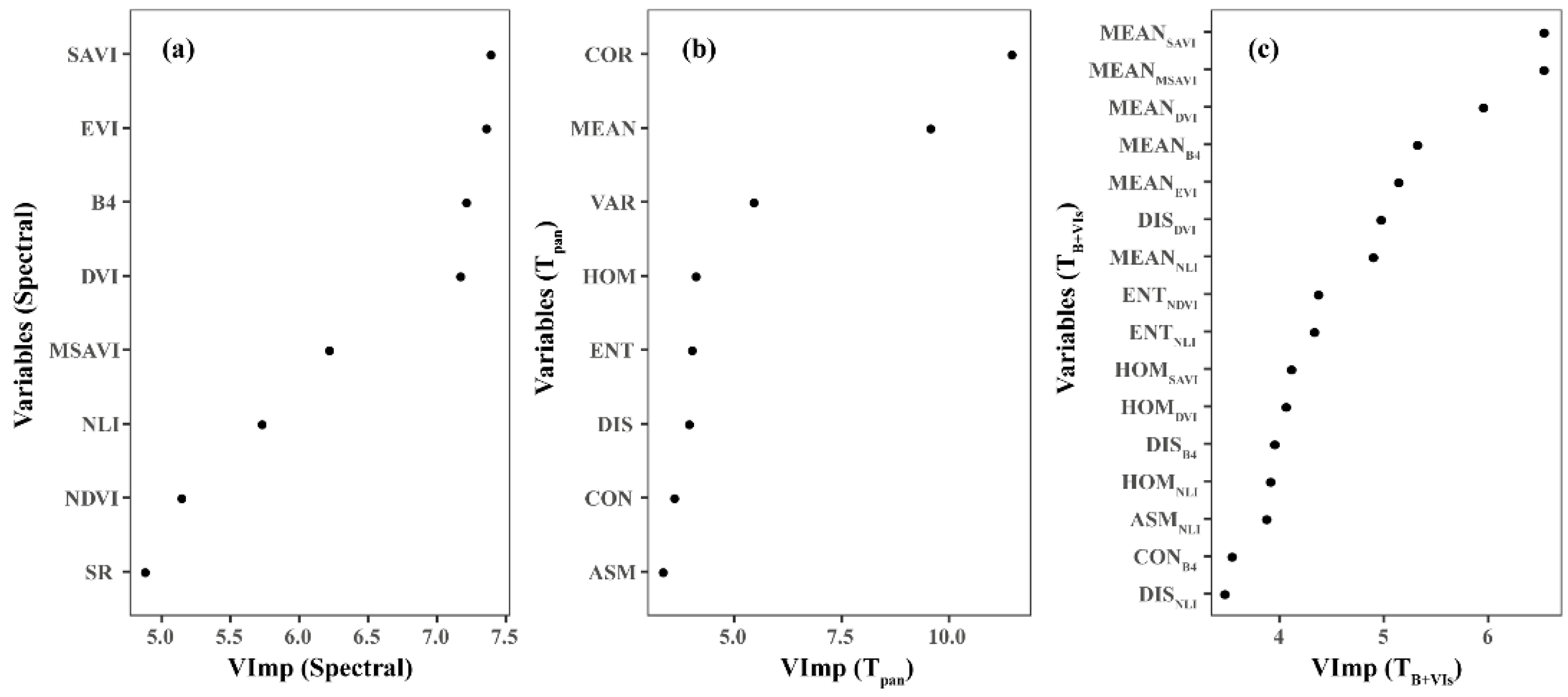
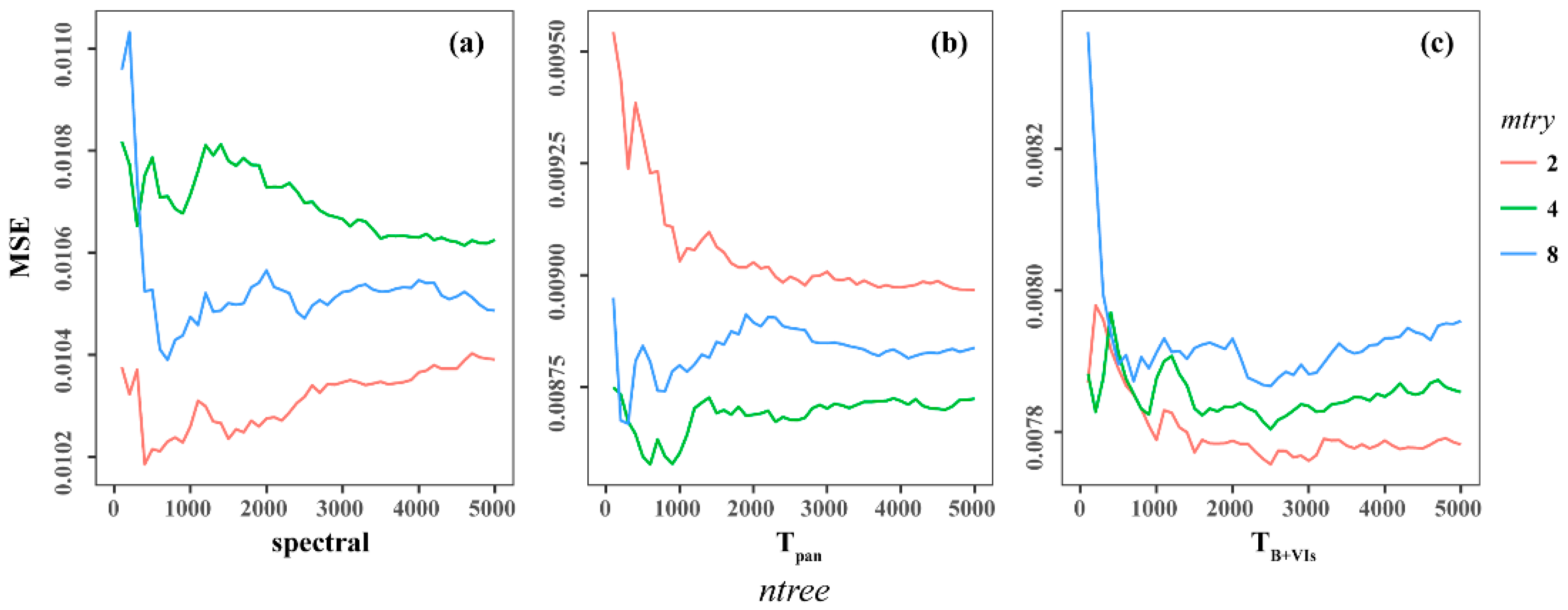
3.2. Variable Selection and Parameter Tuning for the Final Three RF Models

Based on the Boruta algorithm, the explanatory variables that are relevant to the response variables were selected. For Model 1, the optimal number of explanatory variables was eight. In the selected spectral variables, SAVI had the highest importance value. In addition, the EVI, B4 and DVI also had relatively higher values than other spectral variables (Figure 3a). Model 2 was performed based on T_pan with a 15 × 15 window size. All the eight texture measures were selected as relevant variables, and the COR and MEAN hold higher importance values than other texture measures (Figure 3b). Model 3 was performed based on a 9 × 9 window size, and the optimal number of variables was 16. The top five variables in the variable importance were calculated based on the MEAN texture measure (Figure 3c). The MEAN measure calculated from SAVI (MEAN_SAVI) and MSAVI (MEAN_MSAVI) had higher importance values than that of the other variables.

The results indicated that 8, 8, and 16 relevant variables were included in Model 1, Model 2, and Model 3, respectively. Considering the selection rules of mtry [57] and the selected number of explanatory variables in the three RF models, we considered three values for mtry: 2, 4, and 8. After tuning the RF models, the optimal parameters for Model 1 were mtry equal to 2 and ntree equal to 400 (Figure 4a), for Model 2 were mtry equal to 4 and ntree equal to 600 (Figure 4b), and for Model 3 were mtry equal to 2 and ntree equal to 2500 (Figure 4c).

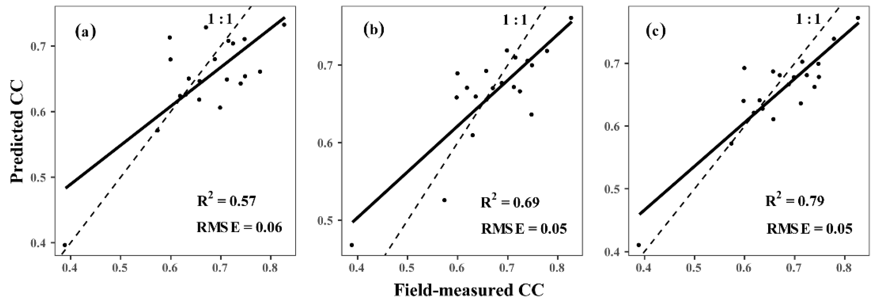
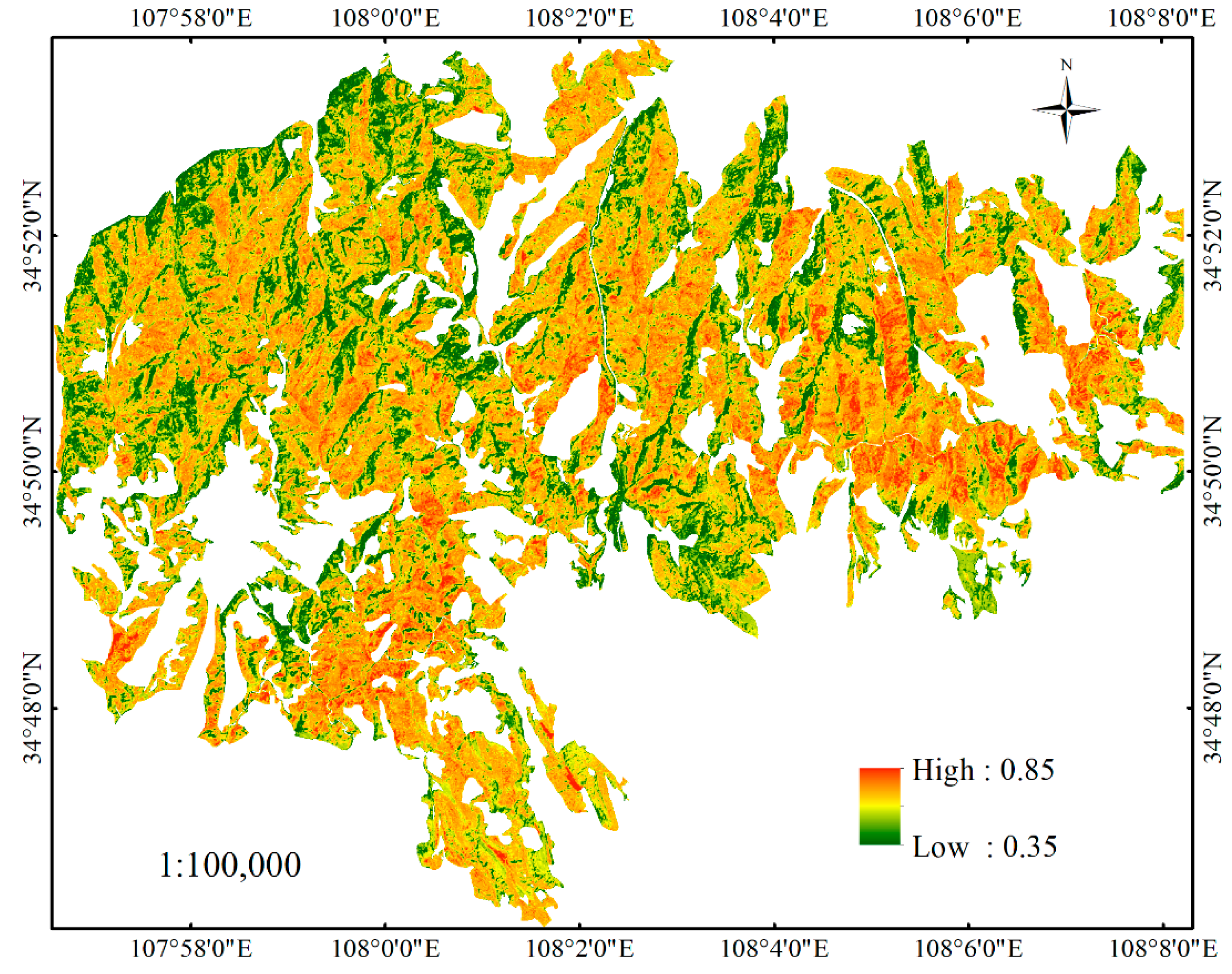
3.3. Model Comparison and CC Mapping

Satisfactory agreement was observed when the remaining 30% of the validation field data were compared with the satellite image predicted data. Figure 5 shows the estimated accuracy of the final three RF models. Model 1 with spectral variables presented the lowest accuracy (R² = 0.57, RMSE = 0.06, Figure 5a), and a higher accuracy was obtained when using T_pan, (R² of 0.69 and RMSE of 0.05, Figure 5b). Model 3 with T_B+VIs had the highest accuracy (R² = 0.79, RMSE = 0.05, Figure 5c). Therefore, Model 3 was used for the final estimation and mapping of the CC of black locust plantations.

The developed RF model (Model 3) was used for calculating pixel-based CC values from the corresponding raster layers of the predictor variables. Figure 6 shows the CC distribution map of the black locust plantations predicted based on Model 3. The eastern region had higher CC values while the western part had lower CC values. In the study area, the average value of CC was approximately 0.6. Most forest CC values were between 0.4 and 0.8, which accounted for more than 99% of the study area (

Table 4. Summary the proportion of CC in different grades.

CC	Percent (%)
<0.4	0.75
0.4–0.6	40.38
0.6–0.8	58.82
0.8–1.0	0.05

). Among these, more than half of the forest CC ranged from 0.6 to 0.8 and 40% of the forest CC were between 0.4 and 0.6.

4. Discussion

The importance of window size has been stressed in evaluations of texture measures [59]. Generally, for the eight GLCM texture measures in the selected seven window sizes, the 15 × 15 window size is optimal for panchromatic image and the 9 × 9 window size is optimal for the spectral variables. Furthermore, the T_B+VIs with 9 × 9 windows obtained higher accuracy than T_pan with 15 × 15 windows. Kamal et al. [60] observed that a pixel window size corresponding to the field plot size or slightly larger could generate high accuracies in LAI estimation. Chen et al. [61] concluded that images at a finer spatial resolution needed a larger window size than at a coarse resolution. In our study, the 15 × 15 window size of T_pan (equivalent to 9 m × 9 m) was still smaller than the sample plot size (20 m × 20 m). For T_B+VIs, the window size of 9 × 9 (equivalent to 21.6 m × 21.6 m), which corresponded to the extent of the field plots, produced higher accuracy than T_pan. This result was consistent with that of Wood et al. [29] and Gomez et al. [59], who suggested that the window size should match the sample plot size to achieve high accuracy.

After filtering the explanatory variables by selecting the optimal window sizes, there are still variables that have a weak relationship with response variable retained. The Boruta algorithm based on RF can select variables that are relevant to the response variables. Wu [62] compared three variable selection methods, i.e., stepwise regression analysis, Pearson correlation analysis, and Boruta algorithm, and found that the Boruta method selected variables capable of obtaining the highest accuracy. Among the spectral variables, the SAVI and EVI were well-correlated with field response variables. The SAVI and EVI could minimize the influences of the soil background, sun angle, and atmosphere [51,63]. Campos et al. [64] compared the performance of SAVI and NDVI in evaluating fraction of ground cover, and found that the SAVI could improve the accuracy, since it was less sensitive to the sun azimuth and row directions. In the aboveground biomass estimation, SAVI showed higher relationship with biomass by adjustment the effect of soil background [65]. Eckert [66] also demonstrated that the EVI is particularly suitable for mapping and monitoring tropical rainforest biomass. Among the four bands, the NIR band was more conducive to CC estimation, and the other three bands were not selected as relevant variables. This result was expected because the NIR band is sensitive to vegetation stress and the chlorophyll content of vegetation [44]. Additionally, NIR reflectance is strong due to the scattering of radiation in the mesophyll cell of leaves and its minimal absorption [23]. However, our study produced only moderately accurate results while using spectral variables, which may have suffered from saturation and multiple layering problems because the CC in our study area was in its peak growth period and had high vegetation cover [26,27].

Compared with spectral variables, the RF model with T_pan presented a significant improvement. All of the texture measures were selected as relevant to the response variables. The eight texture measures explained the variation of CC from different aspects, and only one type of texture measure contained insufficient information to explain the CC variance. Kim [67] demonstrated that adding individual texture measure to spectral bands did not improve forest classification accuracy. However, when incorporated multiple texture measures, the forest classification accuracy increased to 83% in overall accuracy. St.-Louis et al. [6] also found that multiple texture measures explained a higher proportion of the variability in bird species richness than single measures. The higher accuracy of Model 2 was consistent with numerous prior studies, which indicated that T_pan was particularly useful in measuring complex structures, such as tropical forests [29,59]. The usefulness of T_pan may be due to the high resolution of the panchromatic image used for the texture analysis, which increased the scope for distinguishing specific forest structure parameters, especially crown attributes (e.g., CC, crown diameter, etc.) [5,26,27,66].

T_B+VIs yielded the highest accuracy in estimating forest CC compared with the spectral variables and T_pan. The improved performance may be related to their combination of spatial and spectral information, which is consistent with the findings of many previous studies [6,12,27,44,52]. Gu et al. [16], Pfeifer et al. [68], and Pu and Cheng [28] demonstrated that by including texture information into spectral data models, the models’ predictive capacity could be improved, especially for the canopy structure at the stand level, which is mainly because the information associated with spectral and textural signatures is complementary in the estimation of forest parameters [59]. In addition, texture was credible in detecting varying forest canopy structural characteristics and is efficient in addressing saturation problems that are associated with vegetation indices when mapping CC, especially in dense canopies [26].

Our results suggest that QuickBird imagery effectively captured the CC of black locust plantations. The generated map displayed the continuous distribution of CC over a large spatial area (Figure 6), which highlights the convenience of using satellite data for mapping large areas. Such maps can be used to improve the planning and management of tasks, such as land-cover mapping and land-use classification, among others. High CC forests, especially those with a young forest stage, need thinning and pruning to decrease the space and resource competition among individual trees [69]. Young forests with low CC values can lead to enclosures and replanting. Moreover, quantitative maps of forest resources can be used for decision-making by managers and for monitoring a variety of forest inventory parameters, such as forest area changes, biomass accumulation, and health conditions [5,44,68].

Multiple sources of error can lead to uncertainties in forest CC estimation. First, the site CC data were collected and analyzed based on DHPs. To avoid subjective errors when adjusting the threshold, a constant threshold of 128 was used to separate the sky and canopy values. However, the threshold of 128 may not be suitable for all photographs, which may lead to errors in certain photographs. Second, satellite image observations capture an aerial view and obtain the CC by the vertical projection of tree crowns. However, the DHP-obtained CC represented an under the crown measurement and the proportion of sky hemisphere obscured by vegetation when viewed from a single point [70]. This mismatch can be a source of error in the model. Furthermore, shrub and grass in the forest understory will affect the reflectance of the overstory layer, especially in forests with lower CC values [71]. Third, although the satellite images were corrected, errors may remain, and precise co-registration might not be obtained between the images and field plots. Fourth, errors are observed in the RF model itself because the model tends to be overestimated at lower values and underestimated at higher values. However, these errors cannot be avoided. Avitabile and Camia [72] suggest that overestimation may occur in open or young forests while underestimation may be due to the optical saturation under the high biomass of dense forests.

Considering the uncertainties in CC estimation with satellite images, perhaps active sensor and UAV can be used to reduce the effects of these uncertainties in the future. Ma et al. [20] indicated that satellite images were limited by penetration capability in forest area. The active sensors, such as LiDAR and SAR, can penetrate forest canopy and generate vertical structure of vegetation [14,20]. The UAV, which offer high acquisition flexibility and resolution at relatively low costs, have been used to estimate forest cover and basal area successfully [21]. An attractive next step is to using UAV to evaluate forest CC on the Loess Plateau. In addition, the combination of satellite images and UAV or LiDAR is warranted in future research.

5. Conclusions

This study explored the potential use of QuickBird imagery for CC estimations of black locust plantations on the Loess Plateau. We compared the spectral variables, T_pan and T_B+VIs to estimate black locust plantation CC based on RF regression models. The optimal window size for T_pan and T_B+VIs were 15 × 15 and 9 × 9, respectively. The experimental results demonstrated that both T_pan and T_B+VIs performed better than spectral variables. The RF model of T_B+VIs, which reflected the complementary relationship between spectral and textural information, provided the most useful approach to investigating and characterizing black locust plantations CC. This model can be applied for mapping black locust plantations CC on the Loess Plateau of China.

References

1. Jennings, S.B.; Brown, N.D.; Sheil, D. Assessing forest canopies and understorey illumination: Canopy closure, canopy cover and other measures. Forestry 1999, 72, 59–73. [Google Scholar] [CrossRef]
2. Chopping, M.; North, M.; Chen, J.Q.; Schaaf, C.B.; Blair, J.B.; Martonchik, J.V.; Bull, M.A. Forest canopy cover and height from MISR in topographically complex southwestern US landscapes assessed with high quality reference data. IEEE J. Sel. Top. Appl. Earth Obs. Remote Sens. 2012, 5, 44–58. [Google Scholar] [CrossRef]
3. Crowther, T.W.; Glick, H.B.; Covey, K.R.; Bettigole, C.; Maynard, D.S.; Thomas, S.M.; Smith, J.R.; Hintler, G.; Duguid, M.C.; Amatulli, G.; et al. Mapping tree density at a global scale. Nature 2015, 525, 201–205. [Google Scholar] [CrossRef] [PubMed]
4. Gonsamo, A. Leaf area index retrieval using gap fractions obtained from high resolution satellite data: Comparisons of approaches, scales and atmospheric effects. Int. J. Appl. Earth Obs. Geoinf. 2010, 12, 233–248. [Google Scholar] [CrossRef]
5. González-Roglich, M.; Swenson, J.J. Tree cover and carbon mapping of Argentine savannas: Scaling from field to region. Remote Sens. Environ. 2016, 172, 139–147. [Google Scholar] [CrossRef]
6. St-Louis, V.; Pidgeon, A.M.; Radeloff, V.C.; Hawbaker, T.J.; Clayton, M.K. High-resolution image texture as a predictor of bird species richness. Remote Sens. Environ. 2006, 105, 299–312. [Google Scholar] [CrossRef]
7. Peterson, D.W.; Reich, P.B. Fire frequency and tree canopy structure influence plant species diversity in a forest-grassland ecotone. Plant Ecol. 2008, 194, 5–16. [Google Scholar] [CrossRef]
8. Vatandaşlar, C.; Yavuz, M. Modeling cover management factor of RUSLE using very high-resolution satellite imagery in a semiarid watershed. Environ. Earth Sci. 2017, 76, 65. [Google Scholar] [CrossRef]
9. Xiao, J.F. Satellite evidence for significant biophysical consequences of the “Grain for Green” Program on the Loess Plateau in China. J. Geophys. Res. Biogeosci. 2014, 119, 2261–2275. [Google Scholar] [CrossRef]
10. Burner, D.M.; Pote, D.; Ares, A. Management effects on biomass and foliar nutritive value of Robinia pseudoacacia and Gleditsia triacanthos f. inermis in Arkansas, USA. Agrofor. Syst. 2005, 65, 207–214. [Google Scholar] [CrossRef]
11. Zhou, J.J.; Zhao, Z.; Zhao, J.; Zhao, Q.X.; Wang, F.; Wang, H.Z. A comparison of three methods for estimating the LAI of black locust (Robinia pseudoacacia L.) plantations on the Loess Plateau, China. Int. J. Remote Sens. 2014, 35, 171–188. [Google Scholar] [CrossRef]
12. Halperin, J.; LeMay, V.; Coops, N.; Verchot, L.; Marshall, P.; Lochhead, K. Canopy cover estimation in miombo woodlands of Zambia: Comparison of Landsat 8 OLI versus RapidEye imagery using parametric, nonparametric, and semiparametric methods. Remote Sens. Environ. 2016, 179, 170–182. [Google Scholar] [CrossRef]
13. Fang, H.; Li, W.; Wei, S.; Jiang, C. Seasonal variation of leaf area index (LAI) over paddy rice fields in NE China: Intercomparison of destructive sampling, LAI-2200, digital hemispherical photography (DHP), and AccuPAR methods. Agric. For. Meteorol. 2014, 198–199, 126–141. [Google Scholar] [CrossRef]
14. Stojanova, D.; Panov, P.; Gjorgjioski, V.; Kohler, A.; Dzeroski, S. Estimating vegetation height and canopy cover from remotely sensed data with machine learning. Ecol. Inf. 2010, 5, 256–266. [Google Scholar] [CrossRef] [Green Version]
15. Castillo-Santiago, M.A.; Ricker, M.; de Jong, B.H.J. Estimation of tropical forest structure from SPOT-5 satellite images. Int. J. Remote Sens. 2010, 31, 2767–2782. [Google Scholar] [CrossRef]
16. Gu, Z.J.; Ju, W.M.; Li, L.; Li, D.Q.; Liu, Y.B.; Fan, W.L. Using vegetation indices and texture measures to estimate vegetation fractional coverage (VFC) of planted and natural forests in Nanjing City, China. Adv. Space Res. 2013, 51, 1186–1194. [Google Scholar] [CrossRef]
17. Hansen, M.C.; Potapov, P.V.; Moore, R.; Hancher, M.; Turubanova, S.A.; Tyukavina, A.; Thau, D.; Stehman, S.V.; Goetz, S.J.; Loveland, T.R.; et al. High-resolution global maps of 21st-century forest cover change. Science 2013, 342, 850–853. [Google Scholar] [CrossRef] [PubMed]
18. Korhonen, L.; Ali-Sisto, D.; Tokola, T. Tropical forest canopy cover estimation using satellite imagery and airborne lidar reference data. Silva Fenn. 2015, 49. [Google Scholar] [CrossRef]
19. Li, W.; Niu, Z.; Liang, X.; Li, Z.; Huang, N.; Gao, S.; Wang, C.; Muhammad, S. Geostatistical modeling using LiDAR-derived prior knowledge with SPOT-6 data to estimate temperate forest canopy cover and above-ground biomass via stratified random sampling. Int. J. Appl. Earth Obs. Geoinf. 2015, 41, 88–98. [Google Scholar] [CrossRef]
20. Ma, Q.; Su, Y.; Guo, Q. Comparison of canopy cover estimations from airborne LiDAR, aerial imagery, and satellite imagery. IEEE J. Sel. Top. Appl. Earth Obs. Remote Sens. 2017, 10, 4225–4236. [Google Scholar] [CrossRef]
21. Rossi, F.; Fritz, A.; Becker, G. Combining satellite and UAV imagery to delineate forest cover and basal area after mixed-severity fires. Sustainability 2018, 10, 2227. [Google Scholar] [CrossRef]
22. Wallis, C.I.B.; Paulsch, D.; Zeilinger, J.; Silva, B.; Fernandez, G.F.C.; Brandl, R.; Farwig, N.; Bendix, J. Contrasting performance of Lidar and optical texture models in predicting avian diversity in a tropical mountain forest. Remote Sens. Environ. 2016, 174, 223–232. [Google Scholar] [CrossRef]
23. Calvao, T.; Palmeirim, J.M. Mapping Mediterranean scrub with satellite imagery: Biomass estimation and spectral behaviour. Int. J. Remote Sens. 2004, 25, 3113–3126. [Google Scholar] [CrossRef]
24. Karlson, M.; Ostwald, M.; Reese, H.; Sanou, J.; Tankoano, B.; Mattsson, E. Mapping tree canopy cover and aboveground biomass in Sudano-Sahelian woodlands using Landsat 8 and Random Forest. Remote Sens. 2015, 7, 10017–10041. [Google Scholar] [CrossRef]
25. Chasmer, L.; Baker, T.; Carey, S.K.; Straker, J.; Strilesky, S.; Petrone, R. Monitoring ecosystem reclamation recovery using optical remote sensing: Comparison with field measurements and eddy covariance. Sci. Total Environ. 2018, 642, 436–446. [Google Scholar] [CrossRef] [PubMed]
26. Dube, T.; Mutanga, O. Investigating the robustness of the new Landsat-8 Operational Land Imager derived texture metrics in estimating plantation forest aboveground biomass in resource constrained areas. ISPRS J. Photogramm. Remote Sens. 2015, 108, 12–32. [Google Scholar] [CrossRef]
27. Sarker, L.R.; Nichol, J.E. Improved forest biomass estimates using ALOS AVNIR-2 texture indices. Remote Sens. Environ. 2011, 115, 968–977. [Google Scholar] [CrossRef]
28. Pu, R.L.; Cheng, J. Mapping forest leaf area index using reflectance and textural information derived from WorldView-2 imagery in a mixed natural forest area in Florida, US. Int. J. Appl. Earth Obs. Geoinf. 2015, 42, 11–23. [Google Scholar] [CrossRef]
29. Wood, E.M.; Pidgeon, A.M.; Radeloff, V.C.; Keuler, N.S. Image texture as a remotely sensed measure of vegetation structure. Remote Sens. Environ. 2012, 121, 516–526. [Google Scholar] [CrossRef]
30. Tuanmu, M.N.; Walter, J. A global, remote sensing-based characterization of terrestrial habitat heterogeneity for biodiversity and ecosystem modelling. Glob. Ecol. Biogeogr. 2015, 24, 1329–1339. [Google Scholar] [CrossRef]
31. Levesque, J.; King, D.J. Spatial analysis of radiometric fractions from high-resolution multispectral imagery for modelling individual tree crown and forest canopy structure and health. Remote Sens. Environ. 2003, 84, 589–602. [Google Scholar] [CrossRef]
32. Song, L.; Langfelder, P.; Horvath, S. Random generalized linear model: A highly accurate and interpretable ensemble predictor. BMC Bioinform. 2013, 14, 5. [Google Scholar] [CrossRef] [PubMed]
33. Zhang, C.; Denka, S.; Cooper, H.; Mishra, D.R. Quantification of sawgrass marsh aboveground biomass in the coastal everglades using object-based ensemble analysis and Landsat data. Remote Sens. Environ. 2018, 204, 366–379. [Google Scholar] [CrossRef]
34. Ali, I.; Greifeneder, F.; Stamenkovic, J.; Neumann, M.; Notarnicola, C. Review of machine learning approaches for biomass and soil moisture retrievals from remote sensing data. Remote Sens. 2015, 7, 16398–16421. [Google Scholar] [CrossRef]
35. Were, K.; Bui, D.T.; Dick, Ø.B.; Singh, B.R. A comparative assessment of support vector regression, artificial neural networks, and random forests for predicting and mapping soil organic carbon stocks across an Afromontane landscape. Ecol. Indic. 2015, 52, 394–403. [Google Scholar] [CrossRef]
36. Pham, L.T.H.; Brabyn, L. Monitoring mangrove biomass change in Vietnam using SPOT images and an object-based approach combined with machine learning algorithms. ISPRS J. Photogramm. Remote Sens. 2017, 128, 86–97. [Google Scholar] [CrossRef]
37. Belgiu, M.; Drăguţ, L. Random forest in remote sensing: A review of applications and future directions. ISPRS J. Photogramm. Remote Sens. 2016, 114, 24–31. [Google Scholar] [CrossRef]
38. Rodriguez-Galiano, V.F.; Chica-Olmo, M.; Abarca-Hernandez, F.; Atkinson, P.M.; Jeganathan, C. Random forest classification of mediterranean land cover using multi-seasonal imagery and multi-seasonal texture. Remote Sens. Environ. 2012, 121, 93–107. [Google Scholar] [CrossRef]
39. Pullanagari, R.R.; Kereszturi, G.; Yule, I. Integrating airborne hyperspectral, topographic, and soil data for estimating pasture quality using recursive feature elimination with random forest regression. Remote Sens. 2018, 10, 1117. [Google Scholar] [CrossRef]
40. Duro, D.C.; Franklin, S.E.; Dube, M.G. A comparison of pixel-based and object-based image analysis with selected machine learning algorithms for the classification of agricultural landscapes using SPOT-5 HRG imagery. Remote Sens. Environ. 2012, 118, 259–272. [Google Scholar] [CrossRef]
41. Son, N.-T.; Chen, C.-F.; Chen, C.-R.; Minh, V.-Q. Assessment of sentinel-1a data for rice crop classification using random forests and support vector machines. Geocarto Int. 2018, 33, 587–601. [Google Scholar] [CrossRef]
42. Shataee, S.; Kalbi, S.; Fallah, A.; Pelz, D. Forest attribute imputation using machine-learning methods and ASTER data: Comparison of k-NN, SVR and random forest regression algorithms. Int. J. Remote Sens. 2012, 33, 6254–6280. [Google Scholar] [CrossRef]
43. Cracknell, M.J.; Reading, A.M. Geological mapping using remote sensing data: A comparison of five machine learning algorithms, their response to variations in the spatial distribution of training data and the use of explicit spatial information. Comput. Geosci. 2014, 63, 22–33. [Google Scholar] [CrossRef]
44. Wang, H.; Zhao, Y.; Pu, R.L.; Zhang, Z.Z. Mapping Robinia pseudoacacia forest health conditions by using combined spectral, spatial, and textural information extracted from IKONOS imagery and random forest classifier. Remote Sens. 2015, 7, 9020–9044. [Google Scholar] [CrossRef]
45. Frazer, G.W.; Canham, C.; Lertzman, K. Gap Light Analyzer (GLA), Version 2.0: Imaging Software to Extract Canopy Structure and Gap Light Transmission Indices from True-Colour Fisheye Photographs, Users Manual and Program Documentation; Simon Fraser University: Burnaby, BC, Canada; Institute of Ecosystem Studies: Millbrook, NY, USA, 1999; Volume 36. [Google Scholar]
46. Brusa, A.; Bunker, D.E. Increasing the precision of canopy closure estimates from hemispherical photography: Blue channel analysis and under-exposure. Agric. For. Meteorol. 2014, 195, 102–107. [Google Scholar] [CrossRef]
47. Pueschel, P.; Buddenbaum, H.; Hill, J. An efficient approach to standardizing the processing of hemispherical images for the estimation of forest structural attributes. Agric. For. Meteorol. 2012, 160, 1–13. [Google Scholar] [CrossRef]
48. Cescatti, A. Indirect estimates of canopy gap fraction based on the linear conversion of hemispherical photographs-Methodology and comparison with standard thresholding techniques. Agric. For. Meteorol. 2007, 143, 1–12. [Google Scholar] [CrossRef]
49. Nobis, M.; Hunziker, U. Automatic thresholding for hemispherical canopy-photographs based on edge detection. Agric. For. Meteorol. 2005, 128, 243–250. [Google Scholar] [CrossRef]
50. Seidel, D.; Fleck, S.; Leuschner, C. Analyzing forest canopies with ground-based laser scanning: A comparison with hemispherical photography. Agric. For. Meteorol. 2012, 154, 1–8. [Google Scholar] [CrossRef]
51. Huete, A.; Didan, K.; Miura, T.; Rodriguez, E.P.; Gao, X.; Ferreira, L.G. Overview of the radiometric and biophysical performance of the MODIS vegetation indices. Remote Sens. Environ. 2002, 83, 195–213. [Google Scholar] [CrossRef]
52. Haralick, R.M.; Shanmugam, K.; Dinstein, I.H. Textural features for image classification. IEEE Trans. Syst. Man Cybern. Syst. 1973, SMC-3, 610–621. [Google Scholar] [CrossRef]
53. Breiman, L. Random forests. Mach. Learn. 2001, 45, 5–32. [Google Scholar] [CrossRef]
54. Geiß, C.; Aravena Pelizari, P.; Marconcini, M.; Sengara, W.; Edwards, M.; Lakes, T.; Taubenböck, H. Estimation of seismic building structural types using multi-sensor remote sensing and machine learning techniques. ISPRS J. Photogramm. Remote Sens. 2015, 104, 175–188. [Google Scholar] [CrossRef]
55. Cooner, A.J.; Shao, Y.; Campbell, J.B. Detection of urban damage using remote sensing and machine learning algorithms: Revisiting the 2010 Haiti earthquake. Remote Sens. 2016, 8, 868. [Google Scholar] [CrossRef]
56. Kursa, M.B.; Rudnicki, W.R. Feature selection with the Boruta package. J. Stat. Softw. 2010, 36, 1–13. [Google Scholar] [CrossRef]
57. Freeman, E.A.; Moisen, G.G.; Coulston, J.W.; Wilson, B.T. Random forests and stochastic gradient boosting for predicting tree canopy cover: Comparing tuning processes and model performance. Can. J. For. Res. 2016, 46, 323–339. [Google Scholar] [CrossRef]
58. R Core Team. R: A Language and Environment for Statistical Computing; R Foundation for Statistical Computing: Vienna, Austria, 2017. [Google Scholar]
59. Gomez, C.; Wulder, M.A.; Montes, F.; Delgado, J.A. Forest structural diversity characterization in Mediterranean pines of central Spain with QuickBird-2 imagery and canonical correlation analysis. Can. J. Remote Sens. 2011, 37, 628–642. [Google Scholar] [CrossRef]
60. Kamal, M.; Phinn, S.; Johansen, K. Assessment of multi-resolution image data for mangrove leaf area index mapping. Remote Sens. Environ. 2016, 176, 242–254. [Google Scholar] [CrossRef]
61. Chen, D.; Stow, D.A.; Gong, P. Examining the effect of spatial resolution and texture window size on classification accuracy: An urban environment case. Int. J. Remote Sens. 2004, 25, 2177–2192. [Google Scholar] [CrossRef]
62. Wu, C.F. Regional Biomass Estimation and Application Based on Remote Sensing. Ph.D. Thesis, Zhejiang University, Hangzhou, China, 2016. (In Chinese). [Google Scholar]
63. Xue, J.; Su, B. Significant remote sensing vegetation indices: A review of developments and applications. J. Sens. 2017, 2017, 1353691. [Google Scholar] [CrossRef]
64. Campos, I.; Neale, C.M.U.; Lopez, M.-L.; Balbontin, C.; Calera, A. Analyzing the effect of shadow on the relationship between ground cover and vegetation indices by using spectral mixture and radiative transfer models. J. Appl. Remote Sens. 2014, 8, 083562. [Google Scholar] [CrossRef]
65. Yan, F.; Wu, B.; Wang, Y. Estimating aboveground biomass in mu us sandy land using landsat spectral derived vegetation indices over the past 30 years. J. Arid Land 2013, 5, 521–530. [Google Scholar] [CrossRef]
66. Eckert, S. Improved forest biomass and carbon estimations using texture measures from WorldView-2 satellite data. Remote Sens. 2012, 4, 810–829. [Google Scholar] [CrossRef]
67. Kim, M. Object-Based Spatial Classification of Forest Vegetation with IKONOS Imagery. Ph.D. Thesis, University of Georgia, Athens, GA, USA, 2009. [Google Scholar]
68. Pfeifer, M.; Kor, L.; Nilus, R.; Turner, E.; Cusack, J.; Lysenko, I.; Khoo, M.; Chey, V.K.; Chung, A.C.; Ewers, R.M. Mapping the structure of Borneo’s tropical forests across a degradation gradient. Remote Sens. Environ. 2016, 176, 84–97. [Google Scholar] [CrossRef]
69. Liu, J.L.; Yu, Z.Q.; Zhang, S.X.; Wang, D.H.; Zhao, Z. Establishment of forest health assessment system for black locust plantation in Weibei Loess Plateau. J. Northwest A&F Univ. (Nat. Sci. Ed.) 2014, 42, 93–99. (In Chinese) [Google Scholar]
70. Paletto, A.; Tosi, V. Forest canopy cover and canopy closure: Comparison of assessment techniques. Eur. J. For. Res. 2009, 128, 265–272. [Google Scholar] [CrossRef]
71. Hallik, L.; Kull, O.; Nilson, T.; Peñuelas, J. Spectral reflectance of multispecies herbaceous and moss canopies in the boreal forest understory and open field. Can. J. Remote Sens. 2009, 35, 474–485. [Google Scholar] [CrossRef]
72. Avitabile, V.; Camia, A. An assessment of forest biomass maps in Europe using harmonized national statistics and inventory plots. For. Ecol. Manag. 2018, 409, 489–498. [Google Scholar] [CrossRef] [PubMed]
Figure 1. Location of the study area and the field sample plots identified from the multispectral (a) and panchromatic (b) data of QuickBird imagery.
Forests 09 00623 g001
Figure 2. Illustration of the window size effect on the prediction of the forest CC (based on texture calculated from panchromatic image and Band 4).
Forests 09 00623 g002
Figure 3. Number of explanatory variables selected by the Boruta algorithm and their importance values: (a) spectral variables; (b) Tpan; (c) TB+VIs. (VImp represent the variable’s importance values).
Forests 09 00623 g003
Figure 4. Effect of mtry and ntree on the random forest (RF) models of (a) spectral variables; (b) Tpan; (c) TB+VIs.
Forests 09 00623 g004
Figure 5. Plots of the observed and predicted CC using RF with (a) Model 1; (b) Model 2; and, (c) Model 3.
Forests 09 00623 g005
Figure 6. Predicted CC map of the black locust plantations based on Model 3 using QuickBird imagery.
Forests 09 00623 g006