Abstract
In mountain forests of Central Europe, storm and snow breakage as well as bark beetles are the prevailing major disturbances. The complex interrelatedness between climate, disturbance agents, and forest management increases the need for an integrative approach explicitly addressing the multiple interactions between environmental changes, forest management, and disturbance agents to support forest resource managers in adaptive management. Empirical data with a comprehensive coverage for modelling the susceptibility of forests and the impact of disturbance agents are rare, thus making probabilistic models, based on expert knowledge, one of the few modelling approaches that are able to handle uncertainties due to the available information. Bayesian belief networks (BBNs) are a kind of probabilistic graphical model that has become very popular to practitioners and scientists mainly due to considerations of risk and uncertainties. In this contribution, we present a development methodology to define and parameterize BBNs based on expert elicitation and approximation. We modelled storm and bark beetle disturbances agents, analyzed effects of the development methodology on model structure, and evaluated behavior with stand data from Norway spruce (Picea abies (L.) Karst.) forests in southern Austria. The high vulnerability of the case study area according to different disturbance agents makes it particularly suitable for testing the BBN model.
1. Introduction
Extensive areas supporting broad leaf species in warmer and drier lowlands in Central Europe have been transformed to conifer plantations dominated by Norway spruce (Picea abies (L.) Karst.) due to its superior productivity and wood quality compared to the native broad-leaved species [1]. Substantial areas of these secondary coniferous forests are characterized by site properties such as increased frequency of drought periods and gleyic soils where Norway spruce is periodically close to its ecophysiological limits and particularly vulnerable to windthrow and an array of insect and disease organisms. Expected climatic changes with warmer and eventually drier climate in the future will intensify disturbance regimes and affect mountain forests which up until now have provided no suitable habitat for bark beetles due to cool climate [2,3]. Considering risks related to disturbances is therefore a major issue in providing decision support in adaptive forest management. The complex interrelatedness between climate, disturbance agents, and management increases the need for decision support [4,5], especially when designing adaptive forest management strategies to mitigate risks of climate change [6,7].
To prioritize stands for management interventions forest managers need reliable and consistent information on stand susceptibility and expected damages from disturbances. In the forestry domain, various quantitative statistical methods are used to show the influence of disturbance agents on demanded forest products and services [8]. A prerequisite for such approaches is an empirical data base. However, comprehensive empirical data sets including environmental gradients, forest management practices, and information about disturbance agents are rare, which makes the development of statistical models particularly problematic [8,9]. Statistical predictive models (e.g., [10,11]) estimate precise results, especially in domains with low uncertainties on interacting model components. However, the complex causal relationships between disturbance agents, predisposing site and stand-related characteristics, and related damages are well suited for probabilistic models parameterized with qualitative, expert-based knowledge. Such models play an important role in lowering the communication gap between science and decision makers [3]. Varis and Kuikka [12] showed that Bayesian belief networks (BBNs) are well suited to overcome uncertainties from incomplete system knowledge and missing data in decision making, which makes them suitable to deal with a wide range of environmental problems. As BBNs are formal models they can be used to test the implications of specific system drivers analytically [13]. Kolb and Nicholson [14] define BBNs as a graphical structure that allows for the representation and reasoning about an uncertain domain. According to Aguilera et al. [13], BBNs are models defined by a qualitative and a quantitative component. The qualitative component of a Bayesian network uses nodes and arcs to model relationships within a specific domain. Nodes map a set of variables and the arcs indicate the relationship between them, where each node is represented by a finite set of states. For the quantitative component the probability distribution of a certain node is determined by the realized states of its preceding or parent nodes, using a conditional probability table (CPT). The CPTs represent the probability distribution for all possible state combinations relevant for a particular node [14]. The visualization of relations among system elements, combined with the powerful probability theory allowing the incorporation of expert knowledge, increases the applicability for stakeholders and experts [15,16]. The graphical representation makes BBNs easy to understand for end-users and its strong probability theory allows for meaningful knowledge to be elicited via participatory modelling with stakeholders.
In most natural resource management applications BBNs predict the probability of ecological responses to varying environmental, land use, and management drivers [17,18]. However, most of the applications lack the use of a conceptual approach for capturing expert knowledge in modelling uncertainty or risk associated with ecosystem processes. Following Celio et al. [19] and Grêt-Regamey et al. [20], we use a hybrid, expert-based process in BBN parameterization, to combine quantitative and qualitative data, to specify various forest ecosystem service tradeoffs to support management decisions in mountain ecosystems. We combine the BBN development methodology with an innovative approximation method for elicitation of expert knowledge to model highly uncertain interactions of disturbance agents of mountain forests at the stand level scale. We limit the number of considered disturbance agents to spruce bark beetle and storm breakage in order to focus on the knowledge elicitation and parameterization process in model development. We demonstrate the applicability of the BBN model with a regional empirical data set, discuss limitations, and analyze the consequences of using expert knowledge for parameterization on the predictive capacity of the model.
2. Conceptual Framework for BBN Development
There are several practical guidelines for designing a BBN (e.g., [12,17,21,22]). Woodberry et al. [23] presented a theoretical concept for design and implementation of BBNs where domain experts interacted with model experts who provided the methodological frame for the efficient and consistent elicitation of expert knowledge. The approach considered three main steps: (1) structural development, (2) parameter estimation, and (3) quantitative evaluation. Due to the focus on the development process, we capped the number of modeled disturbance agents to two, including a third model to show interactions between them which predicted damages on the stand level scale. Every stage ended with a revised prototype of the BBNs for the bark beetle—and storm breakage—disturbance agents as well as for the damaged trees network. The authors paired up in different roles within the development process. The first author led technical and process-related model development and evaluation as the model expert and the co-authors fulfilled the role of domain experts who contributed expertise in the field of silviculture to support model related elicitation and evaluation. Domain experts participated in steps (1) and (2) of the development process and provided feedback in step (3). Structural development occurred in a workshop setting over the course of three consecutive workshops where domain experts contributed expertise to gather nodes and influence factors of the disturbance related models. While we gathered expert knowledge for step (1) in a workshop setting (see Section 2.1), expert input for step (2) was elicited in an interview format (see Section 2.2).
2.1. Structural Development
For the structural development, the guidelines for developing and updating BBNs in ecological modeling and conservation introduced by Marcot et al. [17] were used in this study. However, in our approach we allowed a connection of a larger number of parent nodes in situations where many influencing characteristics needed to be captured. This may increase realism but in turn also increases the dimensions of the CPT and the related effort to provide the probability estimates. In the first development step an initial causal network that represents causal relationships between knowledge domain variables was designed. Following the suggestions of other studies in environmental contexts (e.g., [24,25]) the BBN was structured into smaller submodels to reduce the complexity. Our approach included two disturbance agent submodels for damages by the spruce bark beetle (Ips typographus sp.) and wind breakage as well as a submodel connecting both disturbance agents in order to predict damages to trees on a stand level scale.
The construction of influence diagrams for each of the three submodels was the first step to show possible influences of several disturbance agents on tree damages on a stand level scale. A forest stand is the basic planning and management unit in forestry and thus in an operational sense is a useful modelling entity. The damage from a disturbance event is related to infested or broken trees which ultimately must be salvaged (i.e., enforced unplanned harvests).
The basic structure of the influence diagrams consists of nodes that represent variables and arrows which indicate the positive or negative influence between them. This type of model was used in the first modeling workshop with domain experts to get an overview of the complexity of the overall problem domain. The first model included damages by the spruce bark beetle and storm breakage as disturbance agents. Interactions between them as well as relationships to damages caused by forest fires and snow were considered in the connecting damaged trees network. In the first workshop the domain experts selected key environmental variables which interact with bark beetle or storm disturbances based on a literature review and the experts’ own expertise. In the subsequent refinement process those main domain variables were arranged in cause–effect relationships that each connected two nodes in the resulting influence diagram. The structure of the influence diagram determines the dependence and independence of relationships among the disturbance agents. As such, without carrying out any numerical calculations it is possible for the experts to identify relevant or irrelevant variables. Figure 1 shows the influence diagram of the damaged trees submodel which links damages of the disturbance agent subnetworks to predict the quantity of damaged trees.
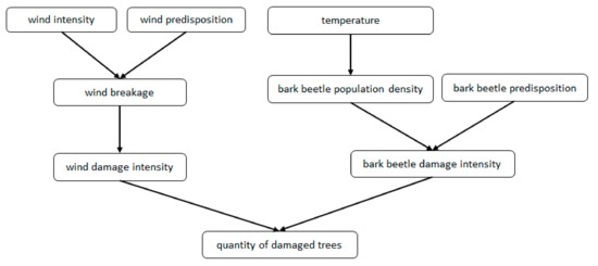
Figure 1.
Influence diagram for the damaged trees network relating wind and bark beetle disturbance agents to predict quantity of damaged tress.
Figure 2 illustrates the bark beetle submodel, including information about the relation (positive or negative influence), as evolved from an initial influence diagram (e.g., Figure 1 of the damaged trees network). Nodes with no incoming arcs indicate input nodes (e.g., “stand age” or “proportion of spruce”) and nodes with no outgoing arcs represent prediction results (e.g., “bark beetle predisposition” for the bark beetle damage model). Results of the damage models show quantities of damage intensity regarding the disturbance agent of each model. The damage quantities represent states to show the likelihood of damage degrees (“single trees”, “group of trees” (damages to more than five trees in a radius of tree length), “horst” (damages > “group of trees” in a scale not more than 0.5 ha in size) and “whole stand”).
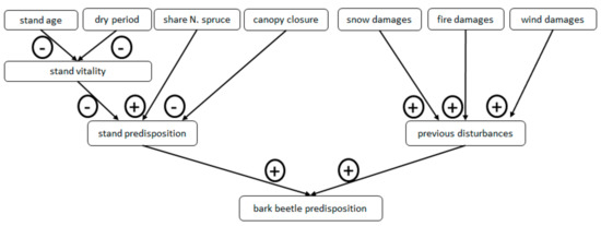
Figure 2.
Influence diagram for the bark beetle disturbance network (“+” and “−“ indicate a positive or negative relation of a pair of nodes, respectively).
Taking a closer look at the node “stand vitality”, the experts identified “stand age” and the number of “dry periods” within a given time frame as relevant causes affecting “stand vitality”. Higher “stand age” and more “dry periods” result in lower states of “stand vitality”. In contrast, high “proportion of spruce” within a stand increases “stand predisposition”. A similar influence diagram was constructed for damages caused by storm breakage. Although the figure of the storm breakage network is not included within this paper, we added some insights into the model evaluation and Supplementary Materials in order to adequately cover considerations regarding it.
In a series of consecutive meetings, all influence diagrams were revised and confirmed in an iterative process between domain and model experts. The influence diagrams were then used to build the prototype BBN structure including state and probability distribution. In this first prototype we relied on expert knowledge to discretize the node states for each influence diagram variable as well as to provide prior probabilities to fill the conditional probability tables for any state combination. Table S1 in the Supplementary Materials shows a full list of BBN nodes including their discrete states. We used the HUGIN Expert decision support tool [26] to implement the BBN prototypes. The decision to use HUGIN as a computer-aided tool to develop BBNs was based on a review of available software packages [1] and on examples from the literature [27,28,29].
2.2. Parameter Estimation
Following Pollino et al. [30], BBNs can be parameterized with both data and knowledge. As detailed empirical data of disturbances and their interrelatedness are mostly lacking [31], a knowledge-based approach supported by silviculture experts was utilized for the calculation of probability tables. In BBN development, the establishment of tables containing the probability for the occurrence of the state categories of nodes is a resource demanding task. Particularly in our approach, where we did not limit the number of parent nodes, this imposed the need for an efficient method to elicit expert judgments codified into the CPTs of each BBN node. The EBBN method (elicitation method for BBNs) described in Wisse et al. [32] was used to provide input to the CPTs using an approximation for the elicitation values. EBBN requires only a limited amount of probability assessments to determine a variable’s full CPT using piecewise linear interpolation. The states of a variable are ordered and the states of each of its parent nodes can be ordered with respect to the influence they exercise.
The EEBN elicitation defines a piecewise linear function f(i) (4). Each assignment a (1) represents the probability for a given scenario of specific state combinations of all parent nodes pa(Xc).
The influence is split up into two components. The joint influence factor ijoint (2) and (3) represents an assignment where all parent nodes pa(Xc) are in a state so as to maximize the positive and negative influences, respectively. An individual influence factor ik underlines the positive or negative influence of each parent node with respect to the joint influence factor ijoint.
In this context, EBBN uses characteristic combinations of states of the parent nodes for the approximation of the full CPTs of the following node [32]. The use of the approximation technique allows the method to limit the number of assignments for expert elicitation.
In this study, experts were asked to (i) order all states of each node in ascending order, so that the most positive state has the highest order and the most negative state has the lowest order; (ii) define the type of influence (positive or negative) of a node on the connecting node; (iii) validate the assignments used within the approximation; and (iv) elicit probability values with respect to those assignments.
The experts defined best guess assignments to represent the characteristic functions that best fit the representation of one state of the elicitation node. A minimum set of assignments was generated and experts were asked to provide the related probabilities. Weights can be used to indicate the distance of the expert’s profession to the analyzed knowledge domain. We used an equally distributed weight to indicate that both experts in our example shared similar domain knowledge. Then the weighted average of the expert judgements normalized to the interval (0, 1) was calculated.
The open source programming language R was used to approximate CPT entries of the BBN based on inputs provided by the EBBN method. Expert elicited values describe the inflection points of the piecewise linear approximation and their weightings corresponding to the importance of one node within the relationship.
The EBBN elicitation process was implemented for the bark beetle and the storm damage disturbance submodel as well as for the damaged trees network. To illustrate an example, the tasks related to the node “stand vitality” of the bark beetle submodel is demonstrated (compare Figure 2). First, the experts ordered the state of the node “stand age” from “>100” to “<60”, where experts defined the state “>100” as the most positive and the state “<60” as the most negative state with regard to stand vitality under the premise of bark beetle infestations. Second, the experts defined whether the influence is positive or negative. For “stand vitality”, both connected nodes are negatively related, so that high stand age or a high number of dry periods result in low stand vitalities. Third, a set of scenarios was defined which represent a minimum set of state combinations to elicit the sections of the approximated function for each cause–effect relation in the BBN. The EBBN algorithm demands one assignment for each “stand vitality” state and two additional assignments for “stand age” and “dry period” to elicit the weight which indicates the importance of the node within the cause–effect relation. For example, to elicit the probability of the most negative “stand vitality” state (alow) experts had to identify the assignment where “stand age” and “dry period” were in their most positive values (“stand age” is in the state “>100 years” and “dry period” in its state “2 periods”).
Based on the elicitations by the experts, approximations for each network node, except the input nodes, were generated using the EBBN algorithm (compare Figure S1 in the Supplementary Materials). Figure 3 shows two examples of the resulting CPT in graphical form. The marked points in the plot show the elicited minimum set of assignments. Each point on the y-axis, which shows a joint probability value for all connected nodes, results in a specific probability for “stand vitality” or “stand stability” for each of its states. The figure indicates elicited probability distributions including associated states of selected nodes. The graph for the node “stand vitality” shows that with a joint probability >f0.6 the probability of the state “very high” increases while the other two states decrease due to the state combinations of the input notes.
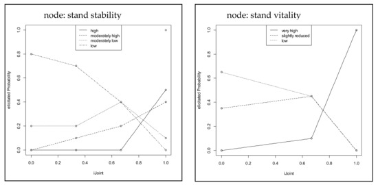
Figure 3.
Conditional probability table (CPT) approximation graphs of two nodes of the bark beetle damage submodel (stand stability and stand vitality).
The CPTs derived by the EBBN algorithm were implemented within the HUGIN environment. As such, for any combination of input states the resulting probabilities for the states of the output node can be computed.
2.3. Model Evaluation
To ensure careful investigation of the network structure, we conducted a sensitivity analysis and an explorative analysis of model behavior in the evaluation. The results of the sensitivity analysis are shown here and the demonstration of the model behavior is presented in the case study application.
The process of model development in BBN modelling recommends two types of sensitivity analyses. Sensitivity to parameters is used to estimate sensitivity of predictions to parameter changes, and sensitivity to findings is utilized to show influences on one node if there is evidence on another parent node [13]. To ensure careful investigation of the network structure, we considered both effects and performed the analysis for each end node of the BBN submodels (“bark beetle damage model” and “storm damage model”) and for the end node of the main model (“tree damage model”).
Figure 4 shows the sensitivity of each node of the bark beetle damage submodel with regard to changes in single CPT values. The x-axis defines the value of sensitivity. The bars to the left show minimal (negative) sensitivities and the bars to the right indicate maximum sensitivities. HUGIN uses minimum and maximum values ranging from negative to positive values to allow for the calculation of average sensitivities. Low sensitivities indicate robust network structures and changes in probability values have only low influence on predictions. In general, the sensitivity analysis of the bark beetle damage submodel shows only low to moderate sensitivities for all connected nodes. The highest sensitivity comes with the node “share of N. spruce”, followed by “canopy closure”.
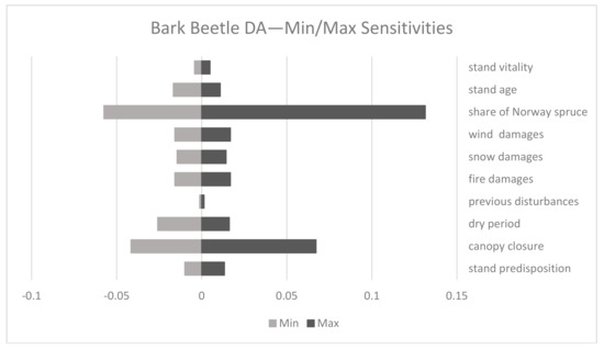
Figure 4.
Sensitivity of each node of the bark beetle damage submodel. “Share of Norway spruce” shows the highest sensitivities (Min = −0.058; Max = 0.131).
Figure 5 shows the sensitivities of the storm damage submodel (structure not shown here) to allow for an interpretation of the sensitivity effects in the damaged trees network. Figure 6 shows evidence of minimum and maximum sensitivity results for the overall model (damaged trees submodel) where the nodes “bark beetle damage intensity”, “wind damage intensity”, as well as “wind intensity” are the most influential on the overall results.
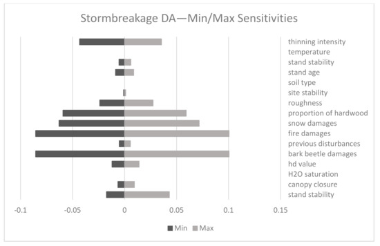
Figure 5.
Sensitivities for the storm damage submodel. “Fire damages” and “bark beetle damages” share the highest sensitivities (Min = −0.085; Max = 0.1).
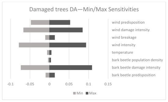
Figure 6.
Sensitivities for the damaged trees network. “Wind damage intensity” shows the highest negative sensitivity (Min = −0.078) while “bark beetle damage intensity” shows the highest positive sensitivity (Max = 0.108).
The domain experts evaluated the plausibility of the BBN models using expert judgment on model response in various scenarios of input gradients within the case study region.
3. Case Study Application
In a case study application, the BBN model was tested for plausibility of predicted probability profiles of the end node categories along a gradient of five demonstration stands. The application case demonstrates how BBNs support decision makers with insights based on scenario analysis. The data for scenario stands A, B, and C for the demo application were taken from a previous study on forest management decision support in lowland conifer forests [33]. The stand data originate from an inner-alpine basin in the south of Austria (14°37′ longitude East, 46°38′ latitude North) with a mean altitude of 550 m. According to Kilian et al. [34], mixed oak forests (Quercus robur L.) with Scots pine, lime (Tilia cordata Mill.), beech (Fagus sylvatica L.), and Norway spruce on acidic soils and admixed hornbeam (Carpinus betulus L.) on calcareous sites constitute the expected natural vegetation composition. The local moniker for the regions is “Dobrova”, which originates from the Slovenian word for oak. Intensive land use for centuries has changed forest composition and currently species composition is dominated by Norway spruce and Scots pine. Both Scots pine and Norway spruce are prone to periodic insect outbreaks (e.g., Neodiprion sertifer Geoffr., Ips typographus L.). Additionally, the forests are frequently damaged by snow breakage due to insufficient or poorly timed stocking control, leading to high height-diameter ratios and eventual breakage. The high vulnerability according to different disturbance agents makes the area particular suitable for testing the BBN model in a case study.
According to Pichler [35], the climate is characterized by cold winters due to temperature inversions, with average January temperatures of −4.6 °C, and hot summers with average July temperatures of 18.5 °C. The annual average temperature is 7.9 °C, and the average annual precipitation in the region ranges from 900–1000 mm of which 500–600 mm fall within the growing season. Soils in the basin are dominated by Cambisols on Pleistocene gravel layers. Depending on the depth to the gravel layer, water supply may be the major limiting factor for tree growth.
Additionally, we designed two extreme state combinations of possible stand parameters to represent the full spectrum of possible input states. Disturbance agent scenarios linking the nodes in their most negative states (with regard to effects on the end node of the submodels) are the so-called “best case” scenario and show the most negative end node probability distribution. Combinations of most positive states represent a “worst case” scenario. The “worst case” and “best case” scenarios result in the lowest and highest possible probability distributions of overall stand damage intensities for the lowest and highest damage classes, respectively. The input parameters for the BBN are listed in Table 1.

Table 1.
Stand data for the case study application.
Figure 7a shows the calculated probabilities for bark beetle predisposition for all four end node states (low, moderately low, moderately high, high) for the five stand types. The results indicate that the BBN predicts lower probabilities of high predisposition states for stand type A and the best case scenario. Older stands with a higher number of annual dry periods and a high share of coniferous trees cause higher probabilities for high bark beetle predispositions.
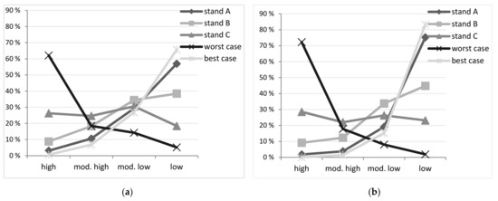
Figure 7.
(a) Probabilities (y-axis) for bark beetle predisposition categories (x-axis) over five stand types; (b) Probabilities (y-axis) for storm damage predisposition categories (x-axis) over five stand types.
Figure 7b indicates the probabilities for storm damage predisposition categories. For the worst case scenario, clearly the highest probability is predicted for the “high” predisposition class, whereas the best case scenario and stand type A show a contrasting result with highest probabilities for the “low” predisposition category. An observation common across both submodels is that stand C shows a quite even probability distribution over all four predisposition categories.
Figure 8 shows the predicted probabilities for the four overall damage intensity classes (whole stand, horst, group of trees, single trees) with regard to the five different stand types. The combined predicted probabilities indicate that only for stand type A and the best case scenario the probabilities for a small number of damaged trees (category “single trees”) is the most likely outcome. Wind intensity under the storm damage agent and the bark beetle population density under the bark beetle damage agent increase the likelihood for higher intensity of damages.
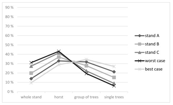
Figure 8.
Probabilities (y-axis) for the damage intensity classes (x-axis) of the overall node “quantity of damage” for the five stand types. Intensities are defined with damage class on stand level scale (where “horst” defines damages > a “group of trees” in a scale not more than 0.5 ha in size and “group of trees” defines damages to more than five trees within a radius of tree length).
4. Discussion
4.1. Model Development
Seidl et al. [31] reviewed various quantitative models to represent complexities within disturbance processes. They concluded that quantitative methods are difficult to apply in situations where only a limited understanding of single and mutual affecting disturbance agents, including bark beetle, exists. Considering the limitation of quantitative methods, we highly focused on a probabilistic BBN approach in two ways. First, BBNs allowed us to use an easily understandable, graph-based visualization to increase freedom in structural development and improve interpretability by end users in decision support. Second, probabilistic methods facilitate model parameterization even in situations of uncertainty.
The bark beetle, storm breakage, and damaged trees networks incorporate uncertainties in BBN model structure as well as their CPT values. Limitations in the understanding of disturbance agents and their interactions lead to relative flat network structures where each node interacts with a relatively high number of parent notes. Although this makes it relatively simple for domain experts to model uncertain interactions, it increases the elicitation burden for each node massively, contradicting with the need of experts not being overwhelmed in the parameterization process. We handled simplicity and efficiency of the parameterization task using the EBBN method [32] to lower elicitation costs using approximation, based on a relative small set of expert input. However, precision of model predictions, especially between inflection points of the linear approximation, depend on validity of the expert elicitation.
4.2. Model Evaluation
The model evaluation in this study included sensitivity analysis and the explorative analysis of model prediction results along gradients of input scenarios to show effects of the development and parameterization method on model behavior. Although model performance testing needs to be done in the future to verify model accuracy, we focus on sensitivity and scenario analyses to draw conclusions on the model development methodology. Due to complex model structures and manifold interactions among system elements it is difficult to anticipate overall model response to specific input vectors during model development. The analysis of model behavior is therefore of particular importance to establish confidence in model predictions and to generate feedback to further model improvement steps.
Sensitivity tests indicate which parts of a complex model structure are particularly relevant for model behavior. This may reveal weaknesses in model structure or identify which input nodes require accurate input data to avoid model predictions which are overly affected by input uncertainty (compare Lexer and Hönninger [36]). Sensitivity tests allowed for the consistency and robustness of internal relationships in the model to be evaluated. The results showed different sensitivities for all nodes of the network with very low sensitivity values in general. In the bark beetle network, nodes with the highest amount of sensitivity are “share of N. spruce” and “canopy closure”. The storm disturbance network is most sensitive to other “previous disturbances” and the overall model is most sensitive to “wind intensity” and “bark beetle damage intensity”. Comparing the magnitude of the sensitivities with findings of other ecology-based BBNs, it becomes evident that the sensitivities of the disturbance agent BBNs are significantly lower. In other studies, the networks often drastically limit the number of nodes and states, and most of them are parameterized with data and not by expert elicitation (e.g., [1,9,12]).
Additionally, the structure of the network is able to influence the sensitivities. Broader BBN structures, where every node is affected by a large number of parent nodes, potentially produce lower parameter sensitivities than network trees with a lower degree of directly connected nodes. It is likely that the model structure and elicitation technique are able to cause low sensitivity values. The weight of a node decreases with its distance in the hierarchy [19].
4.3. Model Justification
To justify predictions of the developed BBN we generated test cases based on a former study in lowland conifer forests by Lexer et al. [33]. Different stand types were used to explore the behavior of the BBN and to discuss plausibility of model predictions in the context of evidence from the scientific literature. In general, findings in the scientific literature match well with the behavior of the BBN model and thus confirm the cause–effect relationships within the network structure [8,37]. Worst and best case scenarios, respectively, showed the expected contrasting probability profiles for the predisposition categories in relation to both disturbance agents, bark beetles and storms.
Although we have only used a minimal set of expert-based approximations for model parameterization, the results for bark beetle predisposition compare well with recent empirical studies (e.g., [8,38,39]) which found that high shares of Norway spruce and drought increased the susceptibility for bark beetle infestations. This is further amplified for situations where two or even more insect generations can develop within one growing season [40,41]. Mezei et al. [42] showed that, due to a higher windstorm frequency, higher elevations can cause more damaged trees, which thereby provides more suitable bark beetle breeding habitat. Given suitable thermal conditions this will increase the insect population density and may ultimately lead to increased probabilities for bark beetle damage [43].
In the developed model, the probability for disturbance predisposition is influenced by previous disturbances (compare Klopcic et al. [44]). Therefore, a higher probability of storm damages indicates a higher probability of bark beetle predisposition. While we have this interrelatedness of disturbances considered in the model structure, the current model version does not differentiate among disturbance agents which therefore makes it = difficult to represent specific overall degrees of influence from other disturbance agents. However, distinguishing different agents and combinations thereof would quickly increase the complexity of the BBN structure and the related demand for probability assignments in the model calibration process.
Pasztor et al. [8] showed that forest management is an important determining factor for bark beetle disturbance risks. The scope of our disturbance agent-based models does not directly include the management perspective. However, the characteristics of the stand types (canopy closure, height to diameter ratio (H/D value), species composition) serving as input nodes for the BBN model can be interpreted as a result of former management activities. Thus, the intensity and type of silvicultural prescriptions were considered indirectly and need to be added into the model to allow better usability for end-users. Netherer and Nopp-Mayr [37] confirmed the important relationship between bark beetle disturbances and stand canopy closure. Thom et al. [38] described that older stands with a higher proportion of spruce leads to increased disturbances. However, there is reason to believe that the predisposing effect on bark beetle infestations increase on stand ages >100 years [39].
With the exception of the “best case” scenario, all stand types had the patch size damage intensity class “horst” as the most likely damage category. For the “best case” scenario, the highest probability was calculated for the “group size” damage intensity class. The overall damage intensity profile appeared plausible with highest probability values for the high intensity category in the “worst case” and the low intensity damages for the “best case” scenario. However, differences in probability distributions between the stand types with regard to the end node categories were fairly small.
An interesting result was generated for stand C. The probabilities for the damaged tree categories were very similar to the “worst case” scenario, which differs from the other scenarios where probabilities for the predisposition categories for bark beetle damages and storm damages were fairly even distributed. The large number of nodes in the submodels for bark beetle and storm damage predisposition may have led to the unspecific probability profile for both submodel end nodes (compare Figure S1 in the Supplementary Materials). This leads to the discussion on the implications of the model structure on the results below.
4.4. Limitations of BBN Development
Although Bayesian networks are well suited to codify complex structures with a large number of dependencies, their graphical representation limits their mathematical potential for being practically useful. However, McCann et al. [45] suggested the use of Bayesian networks for modelling complex ecosystems where uncertainty and variability occurs due to their capacity to display causal relationships and cluster the problem domain into smaller solvable subproblems. We organized our model into three submodels to capture the complex domain of the bark beetle and storm disturbance agents. Both disturbance agents were included in a top level BBN to predict probabilities for damages caused by the agents at a stand level scale. Following the model engineering process, the final influence diagrams show two general characteristics: (i) the number of incoming connections is high for some intermediate nodes and (ii) the network depth increases within higher levels of detail.
Experts adjusted the influence diagram in regard to these domain characteristics. To avoid inconsistency in parameterization and to handle high sensitivities in the ecological domain, we used a weighting of expert inputs [46]. We decided not to lower or limit the number of parent nodes to keep the flexibility as high as possible. This comes into account if reengineering Bayesian networks on a basis of existing predisposition systems that include a wide range of characteristics and calculate one predisposition value based on a set of independent attributes. Pitchforth and Mengersen [47] also agreed that the number of nodes may vary with the problem domain modeled. Due to the fact that the domain experts specified cause–effect relationships for all observed disturbance agents at once, the BBN tended to grow in depth very fast. To lower the complexity and increase the understandability, the experts decided to represent every disturbance agent in independent submodels. Therefore, the final influence diagram connected two separate models (for bark beetle and storm damages) to imply a higher network depth for the damaged trees model.
Expert feedback on parameter estimation showed that the elicitation of assignments with a large number of involved states was a demanding and time-consuming task. Especially with a large number of nodes included in cause–effect relationships, the number of assignments can grow very large. As we used the EBBN method, we were able to minimize the number of required assignments [32]. Complexity in the elicitation process is based on the design and number of the assignments. The size of a constructed assignment depends on the number of states of each linked cause node and the number of states of the effect node. The only way to lower the complexity of assignments within the EBBN method is to limit the number of connected nodes. With the four states used in general to describe the probability output tables, a good compromise between the needed level of detail and resulting complexity was achieved following the feedback of the experts. The EBBN approximation method allows a trade-off to be established between the model’s level of detail and the complexity of the elicitation process for expert driven parameterization. However, our findings indicate that a large number of states and/or nodes within a BBN decrease the absolute importance of single parameter changes, especially when approximation is used. However, sensitivity values could also be affected by the approximation method used to generate a minimum set of assignments. The EBBN method reduces sensitivities, especially by smoothing “outliers” in expert judgments through linear approximation curves. In this case, uncertainties that were solely based on single elicitation values could be minimized. A major driver of sensitivity could be the weightings that we have used to show the importance of single nodes within a connection. On the other hand, wrong elicitation probabilities would yield wrong CPT values for one section of the CPT curve. There is also the need to consider the shape of the approximation curves, as curves with higher gradients might have larger effects on sensitivities than curves with lower gradients. A higher gradient potentially leads to higher variations of successive values within the CTP due to their dependency on the joint approximation curve. The different approximation curves that we have generated during the sensitivity tests indicate gradient variations on a subsection of the curve.
A sensitivity analysis showed that low sensitivities lead to more stable BBN structures where single outliers have fewer effects on prediction results. On the other hand, these sensitivities indicate the need for careful, accurate expert judgment on each elicitation assignment when methods like EBBN are used for the approximation in order to avoid wrong network calibrations. With all these considerations the importance of guidelines [1] for BBN model development becomes more relevant.
5. Conclusions
Process models could be used to provide input for BBN submodels to solve limitations (e.g., construction of feedback loops or continuous system dynamics) in ecosystem development [48]. Statistical models developed from large empirical data sets are often used to discover and describe correlated relationships in forest disturbance regimes (e.g., [8,38]). However, most studies show that a large share of the variation in damage events cannot be explained from empirical data without adding degrees of uncertainty to currently limited understanding [31]. BBNs are becoming popular in forest management decision support for applying an understandable, graph-based representation, which is easy to communicate to a wide range of stakeholders. BBNs assign probabilities to predefined states of each node of the disturbance network structure to handle uncertainties in system understanding and to predict stand level tree damages. Expert feedback showed that the approach allows an easy, first estimate of the model design to be obtained at a reasonable level of complexity. Considering the various scenarios for input variables, Nyberg et al. [49] showed the ability of BBNs to gain evidence on different adaptive management strategies. To highlight these management interactions, future model additions should link input nodes explicitly to forest management prescriptions to show effects on management strategies.
We focused on the BBN model development process and showed a mechanism to minimize elicitation effort to generate full CPTs for their use within a BBN model. The EBBN method [32] allowed an approximation to generate the full CPT from a minimal number of assignments. Further research will have to identify the optimal number of related nodes and states of a BBN model when the EBBN method is used so that elicitation complexity is still manageable. Our design helps to achieve a much more efficient expert elicitation process when time and financial resources are limited. An important point for further consideration is the need to find a balance between the number of nodes that are used within a relationship and the complexity of assignments that need to be generated for the parameterizations task. Parameter sensitivities, in particular, should be further explored to investigate if other approximation algorithms bring better results for parametrizing CPTs. There is also the need to slightly adapt existing guidelines to exceed modeling limitations in order to better handle requirements of specific problem domains. These adaptations may result in an increase of parameterization efforts and modelled complexity but allow a better approximation of real world phenomena.
Model evaluation with sensitivity analysis focuses on analyzing network structure with respect to the effects of the EBBN parameterization method in situations with limited system understanding. The application case investigates the attributes of evaluated networks in real world scenarios, providing good insight into model behavior, and indicating at which nodes attention should be focused in further model improvements. However, predictive accuracy needs to be tested to compare results of quantitative models with outcomes of expert parameterized models. The preparation of a comprehensive model validation data set needs to be addressed in future research.
Supplementary Materials
The following are available online at www.mdpi.com/1999-4907/9/1/15/s1, Figure S1: full list of CPT Approximation graphs for all model nodes, Table S1: node and state definitions of all model nodes.
Acknowledgments
This study was funded by the European FP7 projects FunDivEUROPE (Functional significance of forest biodiversity) and MOTIVE (Models for AdapTIVE forest Management).
Author Contributions
A.R., M.J.L. and H.V. conceived and designed the experiments. A.R. facilitated the model development and elicitation process. A.R., M.J.L. and H.V. developed the model structure. M.J.L. and H.V. performed expert elicitation. A.R. performed the parameterization process. A.R., M.J.L. and H.V. analyzed and interpreted the data. M.J.L. and H.V. contributed materials of the case study application. A.R. drafted the article. A.R., M.J.L. and H.V. critically revised the article.
Conflicts of Interest
The authors declare no conflict of interest.
References
- Spiecker, H.; Hansen, J.; Klimo, E.; Skovsgaard, J.P.; Sterba, H.; Teuffel, K.V. (Eds.) Norway Spruce Conversion—Options and Consequences; EFI Research Report 18; Leiden: Boston, MA, USA, 2004; p. 269. [Google Scholar]
- Seidl, R.; Thom, D.; Kautz, M.; Martin-Benito, D.; Peltoniemi, M.; Vacchiano, G.; Wild, J.; Ascoli, D.; Petr, M.; Honkaniemi, J.; et al. Forest disturbances under climate change. Nat. Clim. Chang. 2017, 7, 395–402. [Google Scholar] [CrossRef] [PubMed]
- Lindner, M.; Fitzgerald, J.B.; Zimmermann, N.E.; Reyer, C.; Delzon, S.; van der Maaten, E.; Schelhaas, M.J.; Lasch, P.; Eggers, J.; van der Maaten-Theunissen, M.; et al. Climate change and European forests: What do we know, what are the uncertainties, and what are the implications for forest management? J. Environ. Manag. 2014, 146, 69–83. [Google Scholar] [CrossRef] [PubMed]
- Lindner, M.; Maroschek, M.; Netherer, S.; Kremer, A.; Barbati, A.; Garcia-Gonzalo, J.; Seidl, R.; Delzon, S.; Corona, P.; Kolström, M.; et al. Climate change impacts, adaptive capacity, and vulnerability of European forest ecosystems. For. Ecol. Manag. 2010, 259, 698–709. [Google Scholar] [CrossRef]
- Vacik, H.; Lexer, M.J. Past, current and future drivers for the development of decision support systems in forest management. Scand. J. For. Res. 2014, 29 (Suppl. 1), S2–S19. [Google Scholar] [CrossRef]
- Keenan, R.J. Climate change impacts and adaptation in forest management: A review. Ann. For. Sci. 2015, 72, 145–167. [Google Scholar] [CrossRef]
- Yousefpour, R.; Jacobsen, J.B.; Thorsen, B.J.; Meilby, H.; Hanewinkel, M.; Oehler, K. A review of decision-making approaches to handle uncertainty and risk in adaptive forest management under climate change. Ann. For. Sci. 2012, 69, 1–15. [Google Scholar] [CrossRef]
- Pasztor, F.; Matulla, C.; Rammer, W.; Lexer, M.J. Drivers of the bark beetle disturbance regime in Alpine forests in Austria. For. Ecol. Manag. 2014, 318, 349–358. [Google Scholar] [CrossRef]
- Hanewinkel, M.; Breidenbach, J.; Neeff, T.; Kublin, E. Seventy-seven years of natural disturbances in a mountain forest area-the influence of storm, snow, and insect damage analysed with a long-term time series. Can. J. For. Res. 2008, 38, 2249–2261. [Google Scholar] [CrossRef]
- Calderon-Aguilera, L.E.; Rivera-Monroy, V.H.; Porter-Bolland, L.; Martínez-Yrízar, A.; Ladah, L.B.; Martínez-Ramos, M.; Alcocer, J.; Santiago-Pérez, A.L.; Hernandez-Arana, H.A.; Reyes-Gómez, V.M.; et al. An assessment of natural and human disturbance effects on Mexican ecosystems: Current trends and research gaps. Biodivers. Conserv. 2012, 21, 589–617. [Google Scholar] [CrossRef]
- Temperli, C.; Bugmann, H.; Elkin, C. Cross-scale interactions among bark beetles, climate change, and wind disturbances: A landscape modeling approach. Ecol. Monogr. 2013, 83, 383–402. [Google Scholar] [CrossRef]
- Varis, O.; Kuikka, S. Learning Bayesian decision analysis by doing: Lessons from environmental and natural resources management. Ecol. Model. 1999, 119, 177–195. [Google Scholar] [CrossRef]
- Aguilera, P.A.; Fernández, A.; Fernández, R.; Rumí, R.; Salmerón, A. Bayesian networks in environmental modelling. Environ. Model. Softw. 2011, 26, 1376–1388. [Google Scholar] [CrossRef]
- Korb, K.B.; Nicholson, A.E. Bayesian artificial intelligence. In Computer Science and Data Analysis; Chapman & Hall/CRC: Boca Raton, FL, USA, 2004. [Google Scholar]
- Cain, J.D.; Jinapala, K.; Makin, I.W.; Somaratna, P.G.; Ariyaratna, B.R.; Perera, L.R. Participatory decision support for agricultural management. A case study from Sri Lanka. Agric. Syst. 2003, 76, 457–482. [Google Scholar] [CrossRef]
- Krueger, T.; Page, T.; Hubacek, K.; Smith, L.; Hiscock, K. The role of expert opinion in environmental modelling. Environ. Model. Softw. 2012, 36, 4–18. [Google Scholar] [CrossRef]
- Marcot, B.G.; Steventon, J.D.; Sutherland, G.D.; McCann, R.K. Guidelines for developing and updating Bayesian belief networks applied to ecological modeling and conservation. Can. J. For. Res. 2006, 36, 3063–3074. [Google Scholar] [CrossRef]
- Ropero, R.F.; Aguilera, P.A.; Fernández, A.; Rumí, R. Regression using hybrid Bayesian networks: Modelling landscape–socioeconomy relationships. Environ. Model. Softw. 2014, 57, 127–137. [Google Scholar] [CrossRef]
- Celio, E.; Koellner, T.; Grêt-Regamey, A. Modeling land use decisions with Bayesian networks: Spatially explicit analysis of driving forces on land use change. Environ. Model. Softw. 2014, 52, 222–233. [Google Scholar] [CrossRef]
- Grêt-Regamey, A.; Brunner, S.H.; Altwegg, J.; Christen, M.; Bebi, P. Integrating expert knowledge into mapping ecosystem services trade-offs for sustainable forest management. Ecol. Soc. 2013, 18, 34. [Google Scholar] [CrossRef]
- Castillo, E.; Gutiérrez, J.M.; Hadi, A.S. Modeling probabilistic networks of discrete and continuous variables. J. Multivar. Anal. 1998, 64, 48–65. [Google Scholar] [CrossRef]
- Cain, J. Planning Improvements in Natural Resource Management. Guidelines for Using Bayesian Networks to Support the Planning and Management of Development Programmes in the Water Sector and Beyond; Centre for Ecology and Hydrology: Bailrigg, UK, 2001. [Google Scholar]
- Woodberry, O.; Nicholson, A.E.; Korb, K.B.; Pollino, C. Parameterising bayesian networks. In AI 2004: Advances in Artificial Intelligence; Springer: Berlin/Heidelberg, Germany, 2005; pp. 1101–1107. [Google Scholar]
- Borsuk, M.E.; Stow, C.A.; Reckhow, K.H. A Bayesian network of eutrophication models for synthesis, prediction, and uncertainty analysis. Ecol. Model. 2004, 173, 219–239. [Google Scholar] [CrossRef]
- Cyr, D.; Gauthier, S.; Etheridge, D.A.; Kayahara, G.J.; Bergeron, Y. A simple Bayesian Belief Network for estimating the proportion of old-forest stands in the Clay Belt of Ontario using the provincial forest inventory. Can. J. For. Res. 2010, 40, 573–584. [Google Scholar] [CrossRef]
- Hugin Researcher™. Hugin Researcher 7.5; Hugin Expert A/S: Gasværksvej, Aalborg, Denmark, 2011. [Google Scholar]
- Bromley, J.; Jackson, N.A.; Clymer, O.J.; Giacomello, A.M.; Jensen, F.V. The use of Hugin® to develop Bayesian networks as an aid to integrated water resource planning. Environ. Model. Softw. 2005, 20, 231–242. [Google Scholar] [CrossRef]
- Henriksen, H.J.; Rasmussen, P.; Brandt, G.; Von Buelow, D.; Jensen, F.V. Public participation modelling using Bayesian networks in management of groundwater contamination. Environ. Model. Softw. 2007, 22, 1101–1113. [Google Scholar] [CrossRef]
- Molina, J.L.; Bromley, J.; García-Aróstegui, J.L.; Sullivan, C.; Benavente, J. Integrated water resources management of overexploited hydrogeological systems using Object-Oriented Bayesian Networks. Environ. Model. Softw. 2010, 25, 383–397. [Google Scholar] [CrossRef]
- Pollino, C.A.; Woodberry, O.; Nicholson, A.; Korb, K.; Hart, B.T. Parameterisation and evaluation of a Bayesian network for use in an ecological risk assessment. Environ. Model. Softw. 2007, 22, 1140–1152. [Google Scholar] [CrossRef]
- Seidl, R.; Fernandes, P.M.; Fonseca, T.F.; Gillet, F.; Jönsson, A.M.; Merganičová, K.; Netherer, S.; Arpaci, A.; Bontemps, J.D.; Bugmann, H.; et al. Modelling natural disturbances in forest ecosystems: A review. Ecol. Model. 2011, 222, 903–924. [Google Scholar] [CrossRef]
- Wisse, B.W.; van Gosliga, S.P.; van Elst, N.P.; Barros, A.I. Relieving the Elicitation Burden of Bayesian Belief Networks; BMA: London, UK, 2008. [Google Scholar]
- Lexer, M.J.; Vacik, H.; Palmetzhofer, D.; Oitzinger, G. A decision support tool to improve forestry extension services for small private landowners in southern Austria. Comput. Electron. Agric. 2005, 49, 81–102. [Google Scholar] [CrossRef]
- Kilian, W.; Müller, F.; Starlinger, F. Die Forstlichen Wuchsgebiete Österreichs. Eine Naturraumgliederung Nach Waldökologischen Gesichtspunkten; Bericht Nr. 82; Forstliche Bundesversuchsanstalt: Wien, Austria, 1994. [Google Scholar]
- Pichler, W. Baumarteneignung und mechanische Stabilität in Kiefernwäldern der Dobrova, Kärnten. Diplomarbeit. Universität für Bodenkultur: Wien, Austria, 2000; p. 138. [Google Scholar]
- Lexer, M.J.; Hönninger, K. Effects of error in model input: Experiments with a forest patch model. Ecol. Model. 2004, 173, 159–176. [Google Scholar] [CrossRef]
- Netherer, S.; Nopp-Mayr, U. Predisposition assessment systems (PAS) as supportive tools in forest management—Rating of site and stand-related hazards of bark beetle infestation in the High Tatra Mountains as an example for system application and verification. For. Ecol. Manag. 2005, 207, 99–107. [Google Scholar] [CrossRef]
- Thom, D.; Seidl, R.; Steyrer, G.; Krehan, H.; Formayer, H. Slow and fast drivers of the natural disturbance regime in Central European forest ecosystems. For. Ecol. Manag. 2013, 307, 293–302. [Google Scholar] [CrossRef]
- Overbeck, M.; Schmidt, M. Modelling infestation risk of Norway spruce by Ips typographus (L.) in the Lower Saxon Harz Mountains (Germany). For. Ecol. Manag. 2012, 266, 115–125. [Google Scholar] [CrossRef]
- Faccoli, M. Effect of weather on Ips typographus (Coleoptera Curculionidae) phenology, voltinism, and associated spruce mortality in the southeastern Alps. Environ. Entomol. 2009, 38, 307–316. [Google Scholar] [CrossRef] [PubMed]
- Baier, P.; Pennerstorfer, J.; Schopf, A. PHENIPS—A comprehensive phenology model for risk assessment of outbreaks of the European spruce bark beetle, Ips typographus (L.)(Col.; Scolytidae). For. Ecol. Manag. 2007, 249, 171–186. [Google Scholar] [CrossRef]
- Mezei, P.; Grodzki, W.; Blaženec, M.; Jakuš, R. Factors influencing the wind–bark beetles’ disturbance system in the course of an Ips typographus outbreak in the Tatra Mountains. For. Ecol. Manag. 2014, 312, 67–77. [Google Scholar] [CrossRef]
- Seidl, R.; Baier, P.; Rammer, W.; Schopf, A.; Lexer, M.J. Modelling tree mortality by bark beetle infestation in Norway spruce forests. Ecol. Model. 2007, 206, 383–399. [Google Scholar] [CrossRef]
- Klopcic, M.; Poljanec, A.; Gartner, A.; Boncina, A. Factors related to natural disturbances in mountain Norway spruce (Picea abies) forests in the Julian Alps. Ecoscience 2009, 16, 48–57. [Google Scholar] [CrossRef]
- McCann, R.K.; Marcot, B.G.; Ellis, R. Bayesian belief networks: Applications in ecology and natural resource management. Can. J. For. Res. 2006, 36, 3053–3062. [Google Scholar] [CrossRef]
- Lucena-Moya, P.; Brawata, R.; Kath, J.; Harrison, E.; ElSawah, S.; Dyer, F. Discretization of continuous predictor variables in Bayesian networks: An ecological threshold approach. Environ. Model. Softw. 2015, 66, 36–45. [Google Scholar] [CrossRef]
- Pitchforth, J.; Mengersen, K. A proposed validation framework for expert elicited Bayesian Networks. Expert Syst. Appl. 2013, 40, 162–167. [Google Scholar] [CrossRef]
- Liedloff, A.C.; Smith, C.S. Predicting a ‘tree change’ in Australia’s tropical savannas: Combining different types of models to understand complex ecosystem behaviour. Ecol. Model. 2010, 221, 2565–2575. [Google Scholar] [CrossRef]
- Nyberg, J.B.; Marcot, B.G.; Sulyma, R. Using Bayesian belief networks in adaptive management. Can. J. For. Res. 2006, 36, 3104–3116. [Google Scholar] [CrossRef]
© 2017 by the authors. Licensee MDPI, Basel, Switzerland. This article is an open access article distributed under the terms and conditions of the Creative Commons Attribution (CC BY) license (http://creativecommons.org/licenses/by/4.0/).