Spatial Autoregressive Models for Stand Top and Stand Mean Height Relationship in Mixed Quercus mongolica Broadleaved Natural Stands of Northeast China

Abstract

The relationship of stand top and stand mean height is important for forest growth and yield modeling, but it has not been explored for natural mixed forests. Observations of stand top and stand mean height can present spatial dependence or autocorrelation, which should be considered in modeling. Simultaneous autoregressive (SAR) models, including spatial lag model (SLM), spatial Durbin model (SDM) and spatial error model (SEM), within nine spatial weight matrices were utilized to model the stand top and stand mean height relationship in the mixed Quercus mongolica Fisch. ex Ledeb. broadleaved natural stands of Northeast China, using ordinary least squares (OLS) as a benchmark model. The results showed that there was a high linear relationship between stand top and stand mean height and that there was a positive spatial autocorrelation pattern in model residuals of OLS. Moreover, SEM and SDM performed better than OLS in terms of reducing the spatial dependence of model residuals and model fitting, regardless of which spatial weight matrix was used. SEM was better than SDM. SLM scarcely reduced the spatial autocorrelation of model residuals. Among nine spatial matrices in SEM, rook contiguous matrix performed best in model fitting, followed by inverse distances raised to the second power (1/d²) and local statistics model matrix (LSM).

1. Introduction

Forest site productivity remains an essential concern in forestry because of its significant role in forest resource availability [1]. Estimating site productivity is crucial to predict forest growth and yield, as well as to maintain sustainable management of forest resources [2,3]. Site index, which is commonly defined as the mean height of dominant and codominant trees of a stand (hereafter referred to as stand top height) at a pre-specified age [4,5,6], has been accepted and widely used as the most expedient indicator of forest site productivity in Germany and North America since around the end of the 19th century because of its simple calculation and efficacious prediction [3,6,7]. Additionally, stand top height is less sensitive to thinning and allows more stability of assessment (e.g., [6,8,9]), and invariance with stand density (e.g., [1,10,11]).

Currently, many foresters have paid increased attention to the estimation of site productivity through site indices based on the national forest inventory (NFI) data [12,13,14,15,16,17,18]. However, NFI data always lack stand top height in some countries, such as China [19,20] and Japan [18]. For instance, three to five average tree heights on each forest plot are measured, and their mean value is regarded as stand mean height in Chinese NFI data, but stand top height in Chinese NFI data is not measured [20]. However, there is a close relationship between stand top height and mean height; therefore, stand top height can be estimated from stand mean height for pure stands by ordinary least squares (OLS), such as a pure stand of European larch, Scots pine, Norway spruce, Chinese Fir, and conifer plantation of Thetford Forest [8,21,22]. To our knowledge, this relationship has not been investigated in the natural mixed stands.

Using OLS to model the relationship of stand top and stand mean height requires the condition that all observations of stand top or stand mean height must be treated as independent units because violation of this assumption could inflate type 1 errors [23,24,25,26,27], lead to biased estimates of the standard errors of model parameters, and decrease the efficiency of estimation in a regression model [28,29,30,31,32]. In reality, each of the stand top or mean height values was derived from different plots that had different locations. Near locations may be more related than distant locations according to the well-known Tobler’s first law of geography [33,34]; that is, the response of a random variable, such as stand top or mean height, in one location is determined by the proximity and weight of its neighboring locations, and this correlation is represented as spatial autocorrelation or dependence [35,36,37].

In recent years, many methods, such as autocovariate models, spatial eigenvector mapping, spatial regression models, spatial generalized estimating equations, etc. [26], have been applied to address spatial autocorrelation in forestry [32,36,37,38,39,40,41,42,43,44,45]. One of these are spatial regression models, which take spatial autocorrelation into account by using spatial weight matrices, including conditional autoregressive (CAR) models and simultaneous autoregressive (SAR) models. The spatial weight matrix of CAR models has to be symmetric, whereas that of SAR models does not need to be symmetric [26]; consequently, SAR models are a better option to use in practice [27,42,44,46,47]. Moreover, SAR models are the most appropriate spatial regression models for fully considering that the autoregressive process occurs in all aspects of models [26,27,42,44] because SAR models have three different forms relying on where the autoregressive process occurs [26,33,47,48], including spatial lag model (SLM), spatial error model (SEM) and spatial Durbin model (or spatial mixed model) (SDM). SLM assumes that the autoregressive process occurs only in the response variable; SEM assumes that the autoregressive process can affect only the error term; and SDM assumes that the autoregressive process are found both in response and explanatory variables. In terms of species distribution, SEM is the most reliable to address spatial autocorrelation, whereas SDM and SLM are weak at reducing spatial dependence [27]. In terms of diameter and height models, which is the most appropriate SAR model depends on specific spatial data structures [42,44]. However, the relationship between stand top and stand mean height using spatial autoregressive models has not yet been investigated. Consequently, it is necessary to investigate the most appropriate technique (SLM, SEM and SDM) in dealing with the spatial dependence of stand top and stand mean height models. Furthermore, spatial weight matrix is a key element in SAR models, thus considering patterns in the response variable that is predicted by neighboring location values rather than by explanatory variables [27]. Many spatial weight matrices have been developed and commonly used, including contiguous neighbors, inverse distances raised to some power, geostatistical matrix and local statistics model (LSM) [44,49].

Therefore, the objectives of this study are (1) to examine the relationship between the stand top height and mean height of mixed Quercus mongolica Fisch. ex Ledeb. broadleaved natural stands and (2) to explore the effects of the inclusion of the spatial autocorrelation in the relationship using SAR models. We selected this mixed stand because it is widely distributed in China, ranging from Heilongjiang province to Jiangsu province (vertical distribution) and from Shandong province to Gansu province (lateral distribution) [50].

2. Data and Methods

2.1. Data

Data were collected from a total of 300 permanent sample plots (PSPs) of natural stands located on the Tazigou state-owned forest farm of Wangqing Forest Bureau in northeast China (129.971°–130.222° E, 43.327°–43.492° N), which is part of Changbai Mountain flora and has a monsoon climate with dry, windy springs and warm, wet summers. The mean annual temperature is approximately 3.9 °C. Mean annual rainfall is 600–700 mm, occurring primarily in the summer. The soil is classified as dark brown forest soil that formed under the combined influences of heat and moisture in mixed forests, and its mean thickness is approximately 40 cm. One-hundred and ninety-nine PSPs were mixed Quercus mongolica broadleaved natural stands and selected for study data. Quercus mongolica in all selected PSPs had the largest basal area proportion; its mean proportion was 46.2%, and its range was from 21% to 64%. In each selected PSP, the major species were Quercus mongolica, Betula platyphylla Sukaczev, Pinus koraiensis Siebold et Zucc., Populus ussuriensis Kom., Acer pictum Thunb. ex Murray and Tilia amurensis Rupr., whereas the minor species included Larix gmelinii (Rupr.) Kuzen., Betula dahurica Pall., Fraxinus mandshurica Rupr., Phellodendron amurense Rupr., Abies nephrolepis (Trautv.) Maxim., Picea asperata Mast. and Juglans mandshurica Maxim. All of the PSPs were established within 12 one hectare large plots in 2013 by the Research Institute of Forest Resources Information Techniques, Chinese Academy of Forestry, and were square in shape (20 × 20 m). All of the standing live trees in each PSP with a diameter at breast height (dbh) equal to or larger than 5.0 cm were marked, tagged, and recorded by species. The total height and dbh of all trees were measured using a Vertext IV electronic measuring device and diameter tape, respectively. Geographic coordinates at the center point of each PSP were acquired using a recreation-grade GPS receiver (Garmin International Inc. Olathe, KS, USA). Summary statistics of stand variables are presented in Table 1.

Table 1. Summary statistics for all selected permanent sample plots (PSPs) (n = 199).

Variable	Mean	SD	Min	Max
Ht (m)	18.38	6.94	12.60	28.38
Hm (m)	10.85	3.00	7.47	17.42
N (stem/ha)	991.3	324.8	375	2275
BA (m2/ha)	20.67	5.77	6.65	35.83
Dg (cm)	16.58	5.65	10.99	24.42

H_t, stand top height; H_m, stand mean height; N, tree number; BA, basal area; Dg, stand average diameter.

Table 1. Summary statistics for all selected permanent sample plots (PSPs) (n = 199).

Variable	Mean	SD	Min	Max
Ht (m)	18.38	6.94	12.60	28.38
Hm (m)	10.85	3.00	7.47	17.42
N (stem/ha)	991.3	324.8	375	2275
BA (m2/ha)	20.67	5.77	6.65	35.83
Dg (cm)	16.58	5.65	10.99	24.42

H_t, stand top height; H_m, stand mean height; N, tree number; BA, basal area; Dg, stand average diameter.

2.2. Stand Top and Stand Mean Height Relationship

The typical top height definition is represented by a specific number of the largest (by height or diameter) trees per unit area represent, e.g., the mean height of the 100 largest trees per hectare [51,52,53]. Regardless of the particular definition of top height employed, the modeling principles involved in projecting stand top height remain essentially the same [53]. Meanwhile, the mean height of the 100 tallest trees per hectare is widely used in China [54] and was applied in this study. Therefore, stand top height was calculated as the arithmetic mean of the four tallest trees according to the 100 tallest trees per hectare, and the selection of the tallest trees did not take into account the species to circumvent the limitation [55] that site index models are difficult to apply in mixed stands, where height estimates of dominant trees must be available for each species in a stand [56]. Stand mean height was determined using Lorey mean height [2,9]. Summary statistics of these two stand variables are presented in Table 1.

A scatterplot of stand top height against stand mean height in 199 selected PSPs is linear in shape (Figure 1), with a high correlation coefficient of 0.847, which was obtained with the function “cor” of the “stats” package in the R statistical language [57]. Therefore, we chose the linear model to fit the relationships of stand top height versus stand mean height as follows:

$$H_t={\beta }_0+{\beta }_1{H}_m+\epsilon$$

(1)

where H_t and H_m denote stand top height and stand mean height, respectively. β₀ and β₁ are both the regression coefficients, and ε is the model error term. Using SLM, SEM and SDM to address spatial autocorrelation, the linear model takes these following forms [33,46,47,48,58,59]:

$$H_t={\beta }_0+\rho W{H}_t+{\beta }_1{H}_m+\epsilon$$

(2)

$$H_t={\beta }_0+{\beta }_1{H}_m+\lambda W\xi +\epsilon$$

(3)

$$H_t={\beta }_0+\rho W{H}_t+{\beta }_1{H}_m+\gamma W{H}_m+\epsilon$$

(4)

where Equation (2) is SLM, Equation (3) is SEM, Equation (4) is SDM, ρ, λ and γ are the spatial autoregressive coefficients, ξ is the spatially dependent error term, ε is the spatially independent error term, W is the spatial weight matrix, and the remaining terms are the same as Equation (1). SLM, SDM and SEM were constructed with the “spdep” package in R [60].

Figure 1. Scatter diagram of stand top height against stand mean height.

Figure 1. Scatter diagram of stand top height against stand mean height.

2.3. Spatial Weight Matrix

Nine spatial weight matrices, including two contiguous neighbors, three inverse distances raised to some power, three geostatistical matrices and LSM, were used in SLM, SEM and SDM.

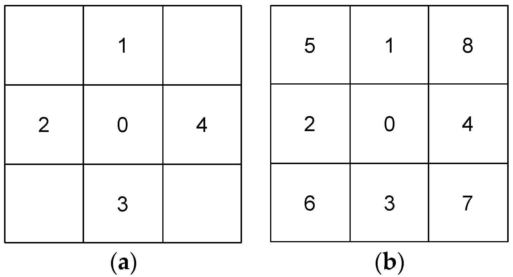
2.3.1. Contiguous Neighbors

Contiguous neighbors include rook contiguity, queen contiguity, Delaunay triangulation neighbors, sphere of influence neighbors, Gabriel graph neighbors and relative graph neighbors. Rook and queen contiguities are commonly used for regular location, whereas the rest of the contiguous neighbors are for irregular location [61]. In this study, rook and queen contiguities were used for our regular study plot. Rook contiguity has four neighbors at each central location in the cardinal directions, and queen contiguity has eight neighbors at each central location in all directions (Figure 2). In Figure 2, cell 0 denotes the central location, cell 1, cell 2, cell 3 and cell 4 denote neighbors of the four cardinal directions, and cell 5, cell 6 cell 7 and cell 8 denote neighbors of the other four directions. Their formulas are as follows [35,62]:

$$w_{ij}=\{\begin{array}{cc}1& \text{within four neighbors}\\ 0& \text{otherwise}\end{array}$$

(5)

$$w_{ij}=\{\begin{array}{cc}1& \text{within eight neighbors}\\ 0& \text{otherwise}\end{array}$$

(6)

where Equation (5) is rook contiguity, Equation (6) is queen contiguity, and w_ij is the spatial weight value of the central location i and its neighbor j. Rook and queen contiguities were constructed with the “spdep” package in R [60].

Figure 2. Schematic diagram. (a) Rook contiguity; (b) Queen contiguity.

Figure 2. Schematic diagram. (a) Rook contiguity; (b) Queen contiguity.

2.3.2. Inverse Distances

Three of the inverse distances were selected, namely, inverse distances raised to one power (1/d), inverse distances raised to the second power (1/d²) and inverse distances raised to the fifth power (1/d⁵). The specific equation is as follows [35,49]:

$$w_{ij}=\{\begin{array}{cc}1/{d_{ij}}^n& \mathrm{if}i\ne j\\ 0& \text{otherwise}\end{array}$$

(7)

where d_ij is the distance between the central location i and its neighbor j, n = 1 is for 1/d, n = 2 is for 1/d², and n = 5 is for 1/d⁵. Three inverse distances were constructed with the “spdep” package in R [60].

2.3.3. Geostatistical Matrix

The autocorrelations of spherical variogram, Gaussian variogram and exponential variogram were defined as the geostatistical matrix under the presumption of intrinsic stationarity [49] and these three geostatistical matrices are currently most commonly used [44,63]. Equation (8) is for spherical variogram (Spher), Equation (9) is for Gaussian variogram (Gaus) and Equation (10) is for exponential variogram (Exp).

$$w_{ij}=\{\begin{array}{cc}1-3d_{ij}/2r-{d_{ij}}^3/2r^3& \mathrm{if}{d}_{\text{ij}}<r\\ 0& \text{otherwise}\end{array}$$

(8)

$$w_{ij}=\{\begin{array}{cc}\exp (-{d_{ij}}^2/r^2)& \mathrm{if}{d}_{\text{ij}}<r\\ 0& \text{otherwise}\end{array}$$

(9)

$$w_{ij}=\{\begin{array}{cc}\exp (-d_{ij}/r)& \mathrm{if}{d}_{\text{ij}}<r\\ 0& \text{otherwise}\end{array}$$

(10)

where r is the range, the remaining terms are as shown in the above equations. Spher, Gaus and Exp were constructed with the “nlme” package in R [64].

2.3.4. Local Statistics Model Matrix

Local statistics model matrix (LSM) was proposed by Getis and Aldstadt [49] based on the G_i * local statistic [65,66]. A positive G_i * indicates that there is high-value clustering around observation I, whereas a negative G_i * indicates low-value clustering. These G_i * values accumulate with increasing distance until these values never rise with distance, implying that any continuity in spatial autocorrelation over distance ends at that distance, which is regarded as the critical distance (d_c), whereas d_c is merely an empirical value because there is no statistical test involved. The specific formula is as follows:

$$w_{ij}=\{\begin{array}{cc}\frac{\left|G_i^{*}(d_c)-G_i^{*}(d_{ij})\right|}{\left|G_i^{*}(d_c)-G_i^{*}(0)\right|}& \mathrm{if}{d}_{\mathrm{c}}>d_{NN1}\mathrm{and}{d}_{\mathrm{i}j}\le d_c\\ \begin{array}{c}1\\ 0\end{array}& \begin{array}{c}\mathrm{if}{d}_{\mathrm{c}}=d_{NN1}\mathrm{and}{d}_{\mathrm{i}j}=d_c\\ \text{otherwise}\end{array}\end{array}$$

(11)

where, d_NN1 is the first nearest neighbor distance for central observation i, G_i *(d_c) is the G_i * score at d_c, G_i *(d_ij) is the G_i * score at d_ij, and G_i *(0) is the G_i * score for ith central observation only. The response variable stand top height has been used as attributed for SLM and SDM, and the model residuals of the OLS model have been used as attributed for SEM to create LSM [44]. LSM was written and constructed based on the “spdep” package in R [60]. All of the spatial weight matrices were row standardized with coding scheme “W” in R [57].

2.4. Test Spatial Autocorrelation of Model Residuals

We selected Moran’s I to test the spatial autocorrelation of model residuals. The formula is as follows:

$$I=\frac{n{\displaystyle \sum _{i=1}^n{\displaystyle \sum _{j=1}^n{w}_{ij}\left(y_i-\overline{y}\right)}}\left(y_j-\overline{y}\right)}{\left({\displaystyle \sum _{i=1}^n{\left(y_i-\overline{y}\right)}^2}\right)\left({\displaystyle \sum {\displaystyle \sum _{i\ne j}{w}_{ij}}}\right)}$$

(12)

where I denotes the Moran’s I of model residuals, n is the number of selected PSPs, y_i and y_j are the model residuals y at PSPs i and j, $\overline{y}$ is the mean of all the model residuals y, and w_ij is the spatial weight matrix between PSPs i and j. The expected value of I under the null hypothesis of no autocorrelation is not equal to zero but given by I₀ = −1/(n − 1). If I is significantly (α = 0.01) greater than I₀, then model residuals y presents positive autocorrelation; otherwise, y presents negative autocorrelation [67]. Moran’s I of model residuals was measured with the function “moran.test” of the “spdep” package in the R statistical language to perform this analysis [60].

2.5. Model Fitting

The spatial autocorrelation patterns of OLS, SLM, SDM and SEM model residuals were compared using correlograms. To identify the best fitting model among OLS, SLM, SDM and SEM, we selected three statistics, i.e., coefficient of determination (R²), root mean square error (RMSE) and Akaike information criterion (AIC), as the approximation criteria. Both R² and RMSE biased only for invalid models with dependent error terms because of these two statistics underlying the assumption of independent observations [37]. AIC can correspond to other goodness of fit measures based on the likelihood function, which does not underlie the assumption of independent error terms [63] and is also heavily influenced by the number of independent variables, penalizing formulations with more independent variables than those with fewer independent variables [49].

3. Results

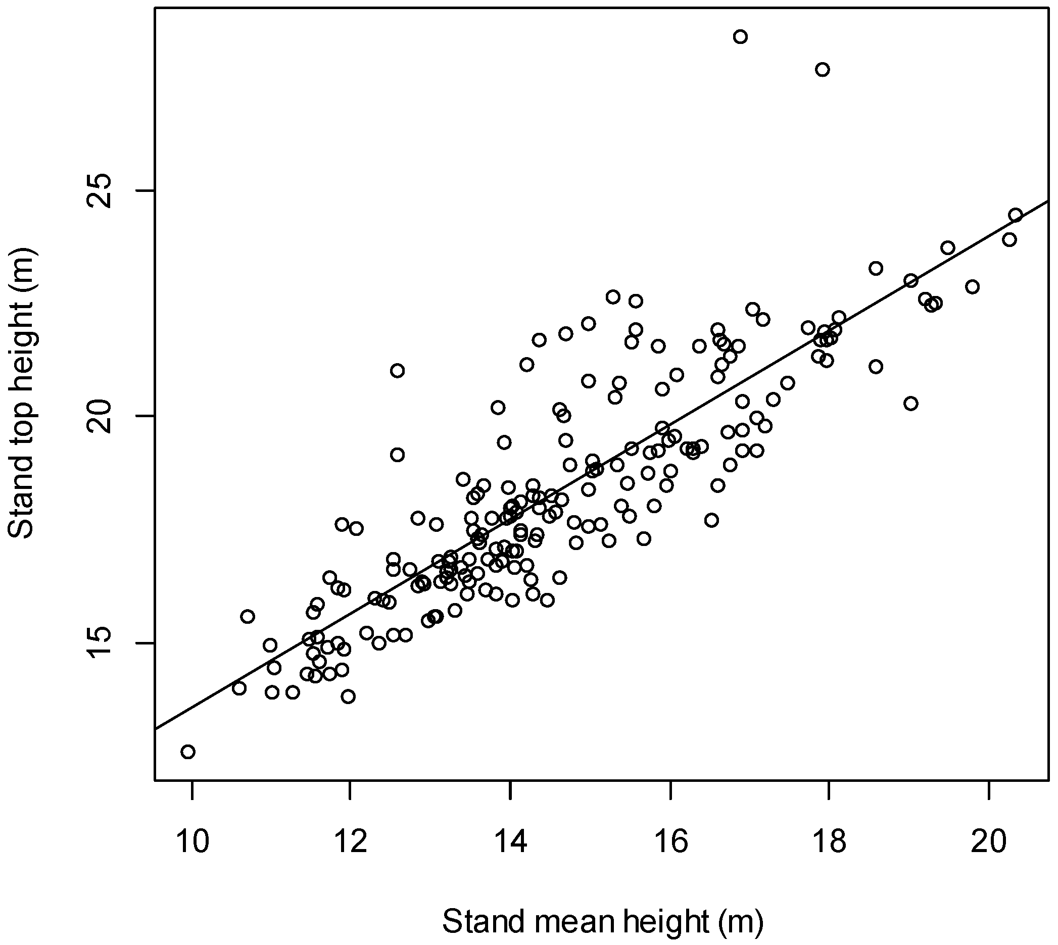
3.1. Relationship between Stand Top and Stand Mean Height

The stand top and stand mean height relationship was modeled by Equation (1). The model coefficients were estimated with OLS, and the coefficients were tested with the T-test. The estimates of the intercept coefficient β₀ and the slope coefficient β₁ were 3.121 (p < 0.001) and 1.043 (p < 0.001), respectively. Their standard errors of β₀ and β₁ were 0.690 and 0.047, respectively.

3.2. Test the Spatial Autocorrelation of Model Residuals

Table 2 shows the Moran’s I of model residuals and a p-value of two-sided with function “moran.test” of the “spdep” package [60] for three SAR models (i.e., SLM, SDM and SEM) against the base model (i.e., OLS) within nine spatial weight matrices. Model residuals of OLS showed a positive spatial autocorrelation pattern because all of Moran’s I were greater than I₀ (I₀ = −1/(199 − 1) = −0.00505) and were significant (p < 0.01) regardless of which spatial weight matrix was used. SEM was the best spatial model to reduce the spatial autocorrelation for the smallest Moran’s I of model residuals and the highest p value, followed by SDM, for each spatial weight matrix, except the 1/d matrix; however, the difference of the 1/d matrix between SDM and SEM was trivial. LSM was the best spatial weight matrix for its Moran’s I closest to I₀ and its p value up to 0.9983, followed by the Spher geostatistical matrix and queen contiguous matrix, whereas the 1/d matrix was the worst. The Moran’s I of SLM residuals was close to that of OLS, implying that SLM almost did a poor job of reducing the spatial dependence because the p-values of seven spatial weight matrices were far less than 0.01, except for 1/d⁵ and Gaus.

Table 2. Moran’s I of four model residuals for nine spatial weight matrices.

W	OLS		SLM		SDM		SEM
	I	p-Value	I	p-Value	I	p-Value	I	p-Value
queen	0.221	0.0018	0.202	0.0040	0.021	0.7143	0.002	0.9171
rook	0.284	0.0004	0.272	0.0007	0.045	0.5420	0.017	0.7874
1/d	0.047	0.0000	0.041	0.0001	0.010	0.2202	0.010	0.2164
1/d2	0.117	0.0000	0.082	0.0034	0.010	0.6204	0.008	0.6586
1/d5	0.162	0.0027	0.079	0.1304	0.012	0.7594	0.006	0.8450
Exp	0.130	0.0001	0.084	0.0079	0.008	0.7050	0.006	0.7365
Gaus	0.151	0.0048	0.070	0.1757	0.012	0.7544	0.005	0.8483
Spher	0.20	0.0026	0.196	0.0038	0.027	0.6410	0.002	0.9198
LSM	0.224	0.0008	0.217	0.0012	0.030	0.6057	−0.005	0.9983

W, spatial weight matrices; I, Moran’s I; Exp, exponential variogram; Gaus, Gaussian variogram; Spher, spherical variogram; LSM, local statistics model matrix.

Table 2. Moran’s I of four model residuals for nine spatial weight matrices.

W	OLS		SLM		SDM		SEM
	I	p-Value	I	p-Value	I	p-Value	I	p-Value
queen	0.221	0.0018	0.202	0.0040	0.021	0.7143	0.002	0.9171
rook	0.284	0.0004	0.272	0.0007	0.045	0.5420	0.017	0.7874
1/d	0.047	0.0000	0.041	0.0001	0.010	0.2202	0.010	0.2164
1/d2	0.117	0.0000	0.082	0.0034	0.010	0.6204	0.008	0.6586
1/d5	0.162	0.0027	0.079	0.1304	0.012	0.7594	0.006	0.8450
Exp	0.130	0.0001	0.084	0.0079	0.008	0.7050	0.006	0.7365
Gaus	0.151	0.0048	0.070	0.1757	0.012	0.7544	0.005	0.8483
Spher	0.20	0.0026	0.196	0.0038	0.027	0.6410	0.002	0.9198
LSM	0.224	0.0008	0.217	0.0012	0.030	0.6057	−0.005	0.9983

W, spatial weight matrices; I, Moran’s I; Exp, exponential variogram; Gaus, Gaussian variogram; Spher, spherical variogram; LSM, local statistics model matrix.

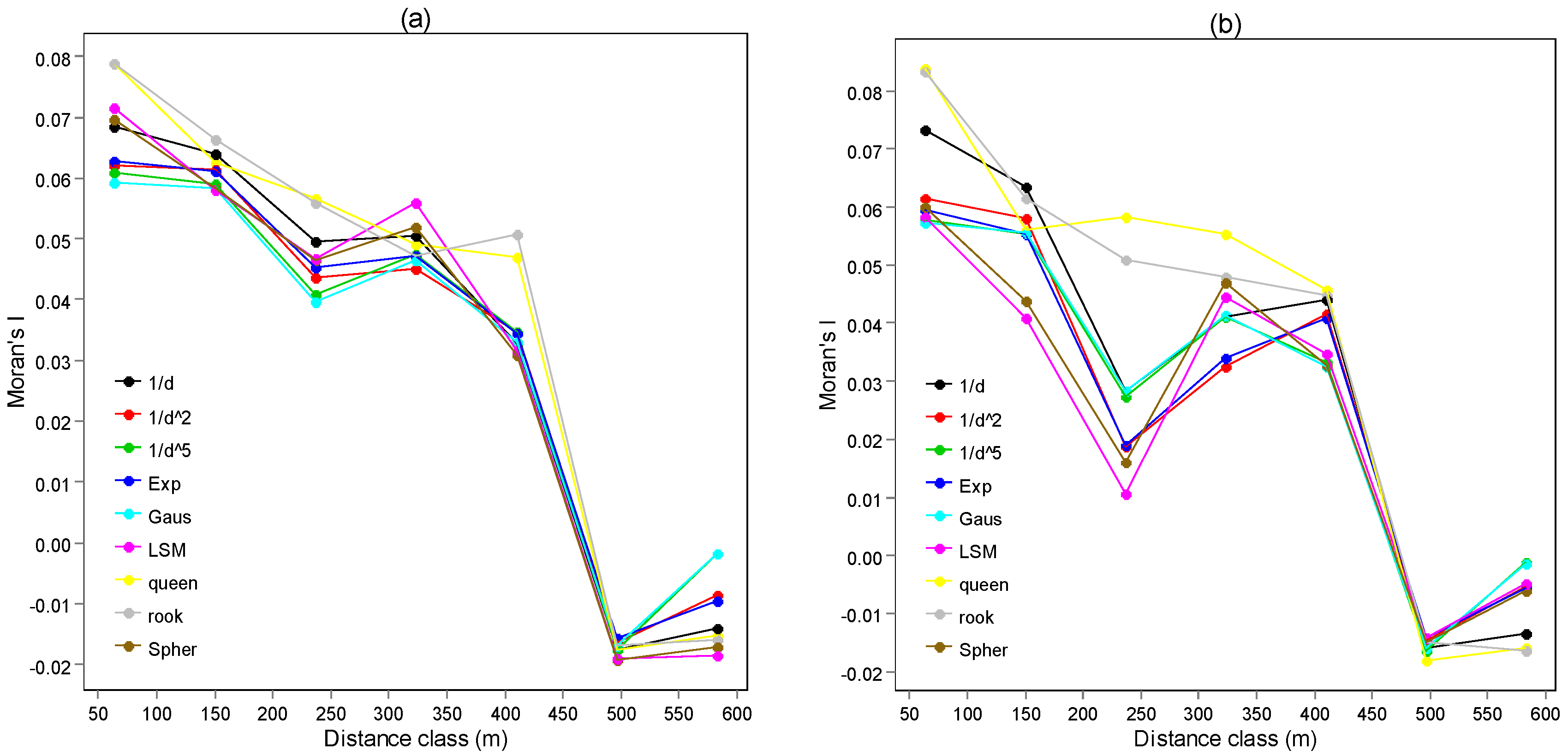
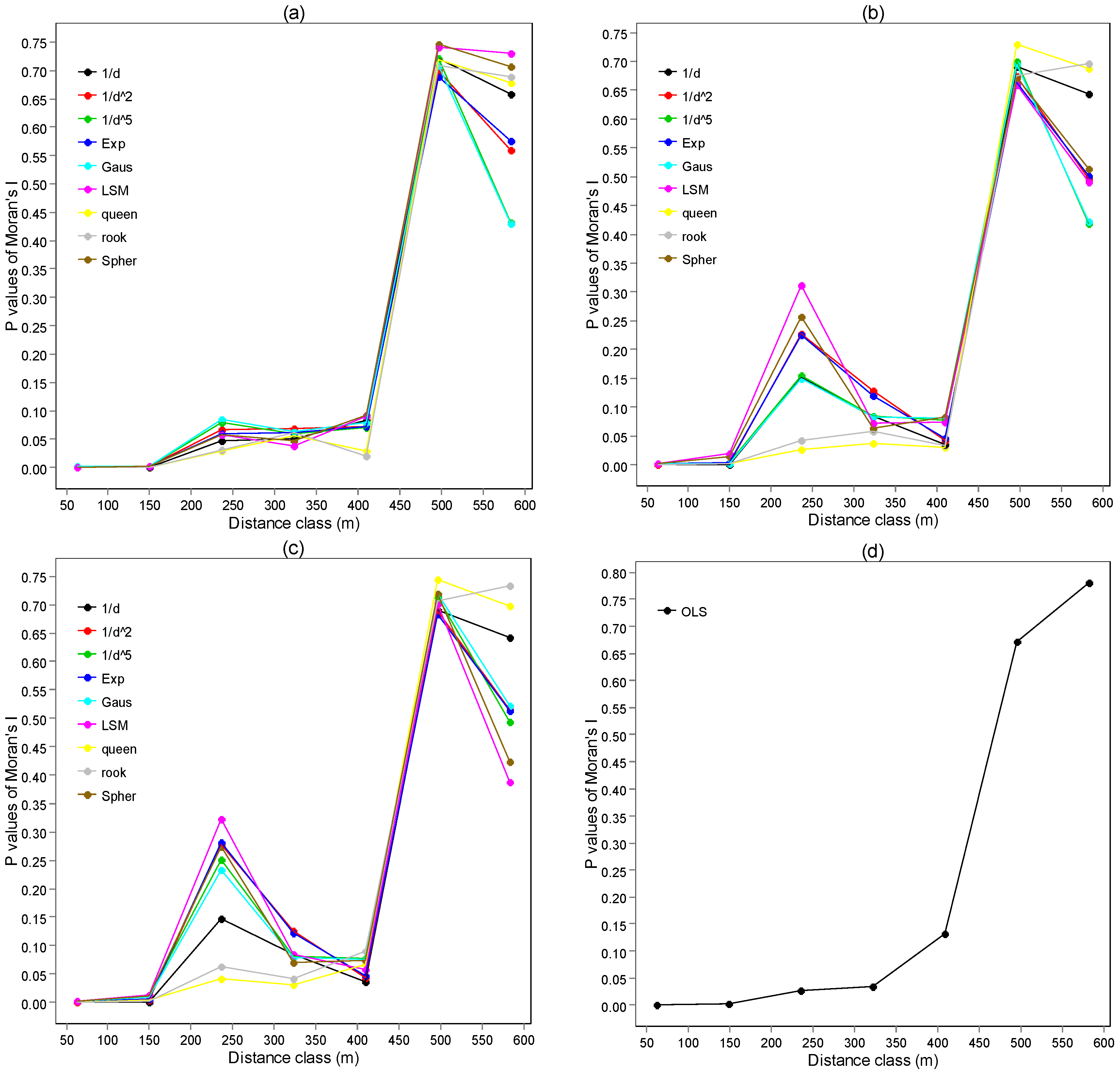
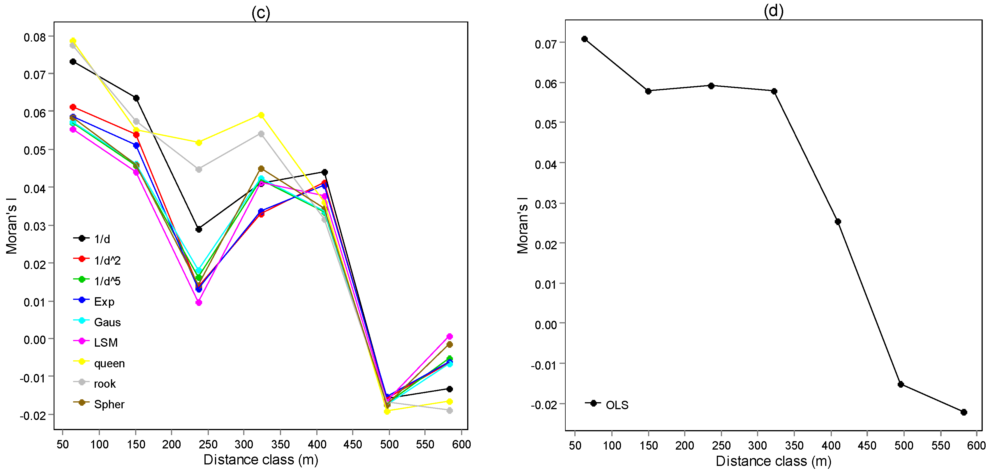
3.3. Spatial Correlogram of Model Residuals

The spatial correlograms of OLS, SLM, SDM and SEM model residuals were constructed with the “pgirmess” package in R [68]. Figure 3 and Figure 4 show the spatial correlograms of model residuals and their p-values for the three SAR models with nine spatial weight matrices and the OLS model. Moran’s I of model residuals were a downtrend, and their p-values were an uptrend with increasing distance class in all models. When distance class increased from 400 m to 500 m, Moran’s I decreased the most, and the p value showed the largest increase. The difference between Moran’s I and I₀ was not significant (p > 0.1) after the distance class of 500 m, indicating that there was no spatial autocorrelation among PSPs when the distance between PSPs was larger than 500 m. Moreover, when the distance class was 250 m, different spatial weight matrices had different performances on reducing spatial dependence in SDM and SEM, whereas there were similar performances with all spatial weight matrices in SLM. LSM was the best spatial matrix to reduce spatial dependence for the lowest Moran’s I and the highest p value, whereas the queen contiguity matrix was the worst in SDM and SEM (Figure 3 and Figure 4).

Figure 3. Correlograms of model residuals using three simultaneous autoregressive (SAR) models with nine spatial weight matrices and the ordinary least squares (OLS) model for (a) spatial lag model; (b) spatial Durbin model; (c) spatial error model; and (d) OLS model.

Figure 3. Correlograms of model residuals using three simultaneous autoregressive (SAR) models with nine spatial weight matrices and the ordinary least squares (OLS) model for (a) spatial lag model; (b) spatial Durbin model; (c) spatial error model; and (d) OLS model.

Figure 4. Diagram of p-values of Moran’s I and distance class using three SAR models with nine spatial weight matrices and the OLS model for (a) spatial lag model; (b) spatial Durbin model; (c) spatial error model; and (d) OLS model.

Figure 4. Diagram of p-values of Moran’s I and distance class using three SAR models with nine spatial weight matrices and the OLS model for (a) spatial lag model; (b) spatial Durbin model; (c) spatial error model; and (d) OLS model.

3.4. Model Fitting

Two SAR models (SDM and SEM) fitted the relationship of stand top and stand mean height better than OLS according to the three criteria, i.e., R², RMSE and AIC, no matter which spatial weight matrix was used. However, SLM was not always better than OLS, which was attributed to AIC within different spatial weight matrices, although the R² and RMSE of SLM were better than those of OLS (Table 3). SEM was slightly better than SDM in AIC. SEM with the rook contiguous matrix is the best model fitting for its highest R², smallest RMSE and lowest AIC, followed by SEM with the 1/d² matrix and SEM with LSM (Table 3). Additionally, when the combination of spatial model incorporated with spatial weight matrix resulted in Moran’s I not being significant (p > 0.1), the R² of the combination was equal or more than 0.73, which was higher than that of OLS, whereas the RMSE and AIC of the combination would be lower than those of OLS (Table 2 and Table 3). This implied that reducing the spatial dependence could improve the model fitting.

Table 3. Model fitting for three spatial autoregressive models.

W	SLM			SDM			SEM
	R2	RMSE	AIC	R2	RMSE	AIC	R2	RMSE	AIC
queen	0.719	1.397	704.880	0.733	1.361	699.851	0.736	1.354	696.609
rook	0.718	1.399	705.258	0.739	1.346	697.043	0.745	1.332	692.527
1/d	0.721	1.393	703.965	0.732	1.365	700.298	0.732	1.365	698.300
1/d2	0.726	1.380	700.548	0.740	1.344	696.125	0.739	1.345	694.419
1/d5	0.730	1.370	698.458	0.736	1.354	698.192	0.734	1.359	697.713
Exp	0.726	1.380	700.490	0.739	1.347	696.649	0.738	1.348	694.947
Gaus	0.730	1.369	698.405	0.735	1.357	698.723	0.732	1.364	698.633
Spher	0.718	1.399	705.502	0.731	1.367	701.003	0.736	1.355	696.863
LSM	0.718	1.400	705.707	0.732	1.364	700.207	0.739	1.345	694.634

W, spatial weight matrices; R², RMSE and AIC of OLS were 0.717, 1.401 and 703.818, respectively.

Table 3. Model fitting for three spatial autoregressive models.

W	SLM			SDM			SEM
	R2	RMSE	AIC	R2	RMSE	AIC	R2	RMSE	AIC
queen	0.719	1.397	704.880	0.733	1.361	699.851	0.736	1.354	696.609
rook	0.718	1.399	705.258	0.739	1.346	697.043	0.745	1.332	692.527
1/d	0.721	1.393	703.965	0.732	1.365	700.298	0.732	1.365	698.300
1/d2	0.726	1.380	700.548	0.740	1.344	696.125	0.739	1.345	694.419
1/d5	0.730	1.370	698.458	0.736	1.354	698.192	0.734	1.359	697.713
Exp	0.726	1.380	700.490	0.739	1.347	696.649	0.738	1.348	694.947
Gaus	0.730	1.369	698.405	0.735	1.357	698.723	0.732	1.364	698.633
Spher	0.718	1.399	705.502	0.731	1.367	701.003	0.736	1.355	696.863
LSM	0.718	1.400	705.707	0.732	1.364	700.207	0.739	1.345	694.634

W, spatial weight matrices; R², RMSE and AIC of OLS were 0.717, 1.401 and 703.818, respectively.

3.5. Model Parameter Estimates

The intercept coefficients β₀ and the slope coefficients β₁ of SLM, SDM and SEM were all estimated and tested by the t-test (Table 4, Table 5 and Table 6), and the autoregressive parameters ρ, γ and λ were all estimated and tested by the likelihood ratio test (Table 7) using the function “lagsarlm” and “errorsarlm” in the “spdep” package [60]. The intercept coefficients β₀ of two spatial models (SLM and SDM) were close to that of OLS and were significant (p < 0.001) in four spatial weight matrices, including the queen contiguous matrix, rook contiguous matrix, Spher geostatistical matrix and LSM, but in the other five spatial weight matrices, the intercept coefficients β₀ were very different and could not reach a significance level of 0.01. Moreover, the intercept coefficients β₀ of SEM were nearly equal to that of OLS and were significant (p < 0.001), regardless of which spatial weight matrix was used. The slope coefficients β₁ of SLM, SDM and SEM were similar to that of OLS and were significant (p < 0.001) for each spatial weight matrix. The standard errors of β₀ and β₁ of SLM, SDM and SEM with nine spatial weight matrices were all equal to or higher than those of OLS (Table 4, Table 5 and Table 6).

Table 4. Model coefficient estimates of SLM for nine spatial weight matrices.

W	β0	Std. Error	z-Value	p-Value	β1	Std. Error	z-Value	p-Value
queen	2.968	0.703	4.224	0.0000	1.031	0.048	21.603	<2.2 × 10−16
rook	2.970	0.715	4.152	0.0000	1.039	0.047	22.299	<2.2 × 10−16
1/d	−1.125	2.657	−0.424	0.6719	0.993	0.057	17.333	<2.2 × 10−16
1/d2	0.947	1.080	0.877	0.3805	0.949	0.061	15.570	<2.2 × 10−16
1/d5	1.770	0.809	2.187	0.0288	0.938	0.059	15.904	<2.2 × 10−16
Exp	1.524	0.927	1.643	0.1003	0.948	0.062	15.370	<2.2 × 10−16
Gaus	1.772	0.807	2.196	0.0281	0.936	0.059	15.853	<2.2 × 10−16
Spher	2.980	0.733	4.068	0.0000	1.039	0.047	22.233	<2.2 × 10−16
LSM	3.064	0.709	4.322	0.0000	1.041	0.047	22.359	<2.2 × 10−16

W, spatial weight matrices.

Table 4. Model coefficient estimates of SLM for nine spatial weight matrices.

W	β0	Std. Error	z-Value	p-Value	β1	Std. Error	z-Value	p-Value
queen	2.968	0.703	4.224	0.0000	1.031	0.048	21.603	<2.2 × 10−16
rook	2.970	0.715	4.152	0.0000	1.039	0.047	22.299	<2.2 × 10−16
1/d	−1.125	2.657	−0.424	0.6719	0.993	0.057	17.333	<2.2 × 10−16
1/d2	0.947	1.080	0.877	0.3805	0.949	0.061	15.570	<2.2 × 10−16
1/d5	1.770	0.809	2.187	0.0288	0.938	0.059	15.904	<2.2 × 10−16
Exp	1.524	0.927	1.643	0.1003	0.948	0.062	15.370	<2.2 × 10−16
Gaus	1.772	0.807	2.196	0.0281	0.936	0.059	15.853	<2.2 × 10−16
Spher	2.980	0.733	4.068	0.0000	1.039	0.047	22.233	<2.2 × 10−16
LSM	3.064	0.709	4.322	0.0000	1.041	0.047	22.359	<2.2 × 10−16

W, spatial weight matrices.

Table 5. Model coefficient estimates of spatial Durbin model (SDM) for nine spatial weight matrices.

W	β0	Std. Error	z-Value	p-Value	β1	Std. Error	z-Value	p-Value
queen	2.743	0.694	3.954	0.0001	1.058	0.048	22.096	<2.2 × 10−16
rook	2.786	0.697	3.996	0.0001	1.060	0.046	23.129	<2.2 × 10−16
1/d	1.046	2.792	0.375	0.7080	1.049	0.061	17.274	<2.2 × 10−16
1/d2	1.303	1.082	1.205	0.2284	1.011	0.064	15.869	<2.2 × 10−16
1/d5	1.917	0.815	2.351	0.0187	0.977	0.064	15.311	<2.2 × 10−16
Exp	1.665	0.921	1.807	0.0708	1.007	0.064	15.669	<2.2 × 10−16
Gaus	1.893	0.814	2.327	0.0200	0.970	0.064	15.121	<2.2 × 10−16
Spher	2.830	0.726	3.895	0.0001	1.058	0.047	22.517	<2.2 × 10−16
LSM	2.849	0.706	4.037	0.0001	1.059	0.047	22.687	<2.2 × 10−16

W, spatial weight matrices.

Table 5. Model coefficient estimates of spatial Durbin model (SDM) for nine spatial weight matrices.

W	β0	Std. Error	z-Value	p-Value	β1	Std. Error	z-Value	p-Value
queen	2.743	0.694	3.954	0.0001	1.058	0.048	22.096	<2.2 × 10−16
rook	2.786	0.697	3.996	0.0001	1.060	0.046	23.129	<2.2 × 10−16
1/d	1.046	2.792	0.375	0.7080	1.049	0.061	17.274	<2.2 × 10−16
1/d2	1.303	1.082	1.205	0.2284	1.011	0.064	15.869	<2.2 × 10−16
1/d5	1.917	0.815	2.351	0.0187	0.977	0.064	15.311	<2.2 × 10−16
Exp	1.665	0.921	1.807	0.0708	1.007	0.064	15.669	<2.2 × 10−16
Gaus	1.893	0.814	2.327	0.0200	0.970	0.064	15.121	<2.2 × 10−16
Spher	2.830	0.726	3.895	0.0001	1.058	0.047	22.517	<2.2 × 10−16
LSM	2.849	0.706	4.037	0.0001	1.059	0.047	22.687	<2.2 × 10−16

W, spatial weight matrices.

Table 6. Model coefficient estimates of SEM for nine spatial weight matrices.

W	β0	Std. Error	z-Value	p-Value	β1	Std. Error	z-Value	p-Value
queen	3.257	0.751	4.335	0.0000	1.033	0.051	20.407	<2.2 × 10−16
rook	3.435	0.751	4.574	0.0000	1.021	0.050	20.256	<2.2 × 10−16
1/d	3.059	0.816	3.748	0.0002	1.047	0.051	20.498	<2.2 × 10−16
1/d2	3.331	0.817	4.078	0.0000	1.029	0.054	18.906	<2.2 × 10−16
1/d5	3.424	0.774	4.423	0.0000	1.023	0.052	19.623	<2.2 × 10−16
Exp	3.381	0.820	4.125	0.0000	1.026	0.055	18.688	<2.2 × 10−16
Gaus	3.430	0.772	4.444	0.0000	1.023	0.052	19.668	<2.2 × 10−16
Spher	3.450	0.762	4.529	0.0000	1.021	0.051	19.949	<2.2 × 10−16
LSM	3.625	0.770	4.707	0.0000	1.009	0.052	19.519	<2.2 × 10−16

W, spatial weight matrices.

Table 6. Model coefficient estimates of SEM for nine spatial weight matrices.

W	β0	Std. Error	z-Value	p-Value	β1	Std. Error	z-Value	p-Value
queen	3.257	0.751	4.335	0.0000	1.033	0.051	20.407	<2.2 × 10−16
rook	3.435	0.751	4.574	0.0000	1.021	0.050	20.256	<2.2 × 10−16
1/d	3.059	0.816	3.748	0.0002	1.047	0.051	20.498	<2.2 × 10−16
1/d2	3.331	0.817	4.078	0.0000	1.029	0.054	18.906	<2.2 × 10−16
1/d5	3.424	0.774	4.423	0.0000	1.023	0.052	19.623	<2.2 × 10−16
Exp	3.381	0.820	4.125	0.0000	1.026	0.055	18.688	<2.2 × 10−16
Gaus	3.430	0.772	4.444	0.0000	1.023	0.052	19.668	<2.2 × 10−16
Spher	3.450	0.762	4.529	0.0000	1.021	0.051	19.949	<2.2 × 10−16
LSM	3.625	0.770	4.707	0.0000	1.009	0.052	19.519	<2.2 × 10−16

W, spatial weight matrices.

Table 7. Estimates of autoregressive parameter for nine spatial weight matrices.

W	SLM		SDM				SEM
	ρ	p-Value	ρ	p-Value	γ	p-Value	λ	p-Value
queen	0.019	0.3327	0.197	0.0049	−0.236	0.0060	0.219	0.0024
rook	0.013	0.4541	0.216	0.0010	−0.267	0.0008	0.250	0.0003
1/d	0.271	0.1734	0.695	0.0074	−0.737	0.0099	0.696	0.0061
1/d2	0.193	0.0217	0.457	0.0007	−0.418	0.0088	0.455	0.0007
1/d5	0.158	0.0067	0.251	0.0033	−0.166	0.1383	0.245	0.0044
Exp	0.163	0.0210	0.392	0.0010	−0.357	0.0113	0.393	0.0010
Gaus	0.159	0.0065	0.240	0.0053	−0.143	0.2017	0.232	0.0074
Spher	0.011	0.5739	0.190	0.0092	−0.233	0.0101	0.229	0.0028
LSM	0.005	0.7382	0.215	0.0059	−0.267	0.0060	0.281	0.0008

W, spatial weight matrices.

Table 7. Estimates of autoregressive parameter for nine spatial weight matrices.

W	SLM		SDM				SEM
	ρ	p-Value	ρ	p-Value	γ	p-Value	λ	p-Value
queen	0.019	0.3327	0.197	0.0049	−0.236	0.0060	0.219	0.0024
rook	0.013	0.4541	0.216	0.0010	−0.267	0.0008	0.250	0.0003
1/d	0.271	0.1734	0.695	0.0074	−0.737	0.0099	0.696	0.0061
1/d2	0.193	0.0217	0.457	0.0007	−0.418	0.0088	0.455	0.0007
1/d5	0.158	0.0067	0.251	0.0033	−0.166	0.1383	0.245	0.0044
Exp	0.163	0.0210	0.392	0.0010	−0.357	0.0113	0.393	0.0010
Gaus	0.159	0.0065	0.240	0.0053	−0.143	0.2017	0.232	0.0074
Spher	0.011	0.5739	0.190	0.0092	−0.233	0.0101	0.229	0.0028
LSM	0.005	0.7382	0.215	0.0059	−0.267	0.0060	0.281	0.0008

W, spatial weight matrices.

It was obvious that different spatial weight matrices and spatial autoregressive models produced very different estimates of the spatial autoregressive parameters (Table 7). Table 7 shows that the estimates of ρ in SLM were less than those in SDM for each spatial weight matrix, although both SDM and SLM had the same spatially lagged response variable WH_t (i.e., the weighted neighboring PSP of stand top height). The estimates of ρ in SLM did not reach the significant level of 0.01, except 1/d⁵ and Gaus, whereas the estimates of ρ in SDM were all significant (p < 0.01), no matter which spatial weight matrix was used. The estimates of γ were negative and significant in five of nine spatial weight matrices. On the other hand, the estimates of λ were positive and significant in all spatial weight matrices (p < 0.01).

4. Discussion

4.1. Spatial Autoregressive Model Selection

Recently, researchers have utilized three spatial autoregressive models (SLM, SDM and SEM) at the plot or stand level and the individual-tree level to reduce the spatial autocorrelation of model residuals [27,42,44]. At the plot or stand level, Kissling and Carl [27] used these models to fit the artificial data that had 1108 cells (10 × 10 m), and the results showed that SEM was the most reliable spatial autoregressive model for reduction of spatial dependence. In individual-tree level, Meng et al. [42] fitted the tree height-diameter relationship in case 1 (49 artificial loblolly pine trees on a 0.049 ha plot) by using these models and showed that SLM was the better than the other two models, whereas in case 2 (a 4.6451 ha plot with 690 slash pine), the results indicated that SEM was superior to SLM and SDM. Lu and Zhang [44] fitted the same relationship as Meng et al. [42], but in a large softwood stand (400 × 200 m) with 3982 trees, showed that SDM was the best, followed by SEM. These previous studies indicate that the performance of spatial autoregressive models depends on the study level and data size.

In this study, we used these spatial models to fit the stand top and stand mean height relationship with 199 selected PSPs (20 × 20 m) in a plot or stand level. Our results showed a similar finding as the studies of Kissling and Carl [27] and Meng et al. [42] in case 2, that SEM was the best spatial autoregressive model to decrease the spatial dependence and improve the model fitting, independent of which spatial weight matrix was used. SDM was close to SEM. SLM was the worst to cope with spatial autocorrelation of model residuals because SLM with seven of nine spatial weight matrices cannot reduce the spatial dependence of model residuals (except 1/d⁵ and Gaus). Moreover, when the difference of Moran’s I of spatial model residuals and the expected value I₀ was not significant (p value was greater than 0.1), the one spatial model was superior to OLS in model fitting because of its higher R², lower RMSE and smaller AIC, regardless of which spatial models and spatial weight matrix were used.

4.2. Model Parameter Estimates

The estimate of model parameter from spatial autoregressive models is a very significant issue in geographical ecology and forestry (e.g., [24,27,69,70]), and biased estimates and incorrect model specifications directly influence hypothesis testing (e.g., [44,69,71]). Lu and Zhang [44] suggested that various spatial weight matrices may induce unequal estimates of model parameters, the intercept coefficients can be affected by the model specifications (e.g., SDM and SLM) and spatial weight matrices, and the estimates of the model coefficient in SEM were very close to those of OLS. Our results confirmed their suggestion. Additionally, the intercept coefficients β₀ in SLM and SDM were similar to those of OLS when SLM or SDM combined with some spatial weight matrix (e.g., queen, rook, Spher and LSM), which enabled β₀ to reach the significance level of 0.001. The standard errors of the model coefficient estimates of OLS were equal or lower than those of the spatial autoregressive models for reducing the spatial autocorrelation, which confirmed the argument of West et al. [29], i.e., when OLS was used to fit the data that contained spatial dependence, the covariance matrix of the parameter estimates was underestimated.

4.3. Spatial Weight Matrices

Getis and Aldstadt [49] created three types of artificial data; each type had 9000 observations (30 × 30 raster) and their spatial patterns were random, two clusters, and six clusters, respectively. Three artificial data were modeled with SLM and nine spatial weight matrices. They concluded that LSM was the best matrix among all of the spatial weight matrices through comparative analysis with AIC, ρ and Moran’s I of model residuals, and geostatistical matrices were the next best generally. However, Lu and Zhang [44] concluded that the LSM was not the best but that geostatistical matrices were superior using large forest stand data, no matter which spatial autoregressive model used.

Our results yielded a similar finding as the study of Getis and Aldstadt [49] as LSM, rather than geostatistical matrices, with SEM performed better than the other eight spatial weight matrices to reduce the spatial autocorrelation of model residuals, followed by Spher geostatistical matrix and queen contiguous. The reason may have resulted from the study level (plot or stand level, individual-tree level) of our study and that of Getis and Aldstadt [49] as both were at the plot or stand level, whereas the study level of Lu and Zhang [44] was at the individual-tree level. However, using the SEM to model the data, rook contiguous matrix, instead of LSM, showed optimal performance in terms of model fitting (maximum R², minimum RMSE and minimum AIC), and LSM and 1/d² were second best. This suggests that the optimal spatial matrix depends on specificity in study data. In terms of model intercept coefficients estimates, five spatial weight matrices, including 1/d (worst), 1/d² (second worst), 1/d⁵, Exp and Gaus, were not significant at a risk level of 0.01 in SLM and SDM, whereas the other four spatial weight matrices (queen, rook, Spher and LSM) did well in SLM and SDM.

4.4. Stand Top and Stand Mean Height Relationship

A high linear correlation between stand top and stand mean height was found in pure plantations as the correlation coefficients of European larch, Scots pine and Norway spruce are 0.994, 0.989 and 0.974, respectively [8], and the correlation coefficient of Chinese fir is 0.995 [21]. However, there was a gap in the relationship for natural mixed forests. In this study, we found that the correlation coefficient in a mixed natural stand was 0.847 and relatively lower than that of pure stands. This difference was mainly due to the complicated species composition. However, Moran’s I of OLS residuals was different, with the expected value I₀ at a significance level of 0.01. We used three SAR models (SLM, SDM and SEM) and had a finding that SEM was the best to reduce spatial dependence, SDM was very close to SEM, and SLM did not adequately account for spatial autocorrelation. SLM incorporates spatial dependence with the WH_t, and SDM considers spatial dependence in both the WH_t and weighted neighboring PSP of stand mean height (called WH_m), and the primary objective of SEM is to achieve more efficient estimators by correcting potential estimated bias affecting spatial autocorrelation due to unobserved spatial variables [42]. Therefore, our finding indicated that stand top height at one PSP is affected not by the spatial variable WH_t but by the combination of the spatial variables WH_t and WH_m. Furthermore, stand top height at one PSP is significantly affected by unobserved spatial variables at neighboring PSPs. In the future, we need to incorporate environmental factors, stand non-spatial structure characteristics and stand spatial structure characteristics into SAR models to further identify which is the most effective for stand top height. In addition to three SAR models, we could incorporate other models dealing with spatial autocorrelation, such as generalized linear mixed models, generalized additive models, spatial eigenvector mapping and Bayesian spatial models in further studies.

Stand top height is a key variable for which to use the site index method that is commonly species dependent, but the site index method has limitations when applying to mixed uneven-aged forests because of difficulties in tree species-specific age measurements and in height estimates that dominant trees must be available for each species [56]. An estimate of stand top height that is independent of species could potentially address this limitation [55]. Raulier et al. [72] used stand top height without accounting for species to compare the different site index curves from different data sources, including permanent sample plots, temporary sample plots and stem analyses. Anyomi et al. [56] used stand top height to study spatial and temporal heterogeneity of forest site productivity drivers within the eastern boreal forests of Canada. Consequently, we used stand top height and mean height without considering species.

In addition, mean height of 100 tallest trees per hectare was regarded as a top height in this study; other definitions of top height may be allowed for further study, such as the mean height of 100 thickest trees per hectare, mean height of a fixed percentage of occurring trees, especially the definition of top height, which considered the plot size selection effect to reduce estimate bias [52]. These definitions of top height may be available in forest inventory.

4.5. Modeling Approach Applications in LiDAR Data and Crown Fire Modeling

Circumvention of time and cost constraints in field-based forest inventory, foresters have increasingly regarded remote sensing data as a means of assisting and complementing, and forest canopy height was retrieved easily using LiDAR data and InSAR [22,73,74,75]. In reality, forest canopy height in a resolution cell is more similar to its nearby resolution cells because they have similar soil, topography, microclimate, etc., that is, there is a spatial autocorrelation between a resolution cell and its nearby cells. Therefore, considering the spatial autocorrelation into forest canopy height from LiDAR could improve the utilization of LiDAR in forest monitoring and forest inventory. Mcroberts [76] reviewed that the k-Nearest Neighbors (kNN) was a suitable approach to deal with spatial autocorrelation and improve the prediction of forest variables those were from most similar, or nearest resolution cells. There are three common selections for spatial weight matrices in kNN, including a constant value of 1, 1/d and 1/d² [76,77,78]. These common spatial weight matrices within kNN were investigated to predict forest canopy height by Mcinerney et al. [74] and the result showed the performances of different spatial weight matrices depended on different k values and different bands. In addition to these common spatial weight matrices, other spatial weight matrices such as 1/d⁵, Gaus, Spher, Exp, queen, rook and LSM, may be suitable for reducing spatial dependence because different nearby resolution cells may generate the different spatial pattern (structure). Meanwhile, SLM could be regarded as an alternative model in height prediction for its assumption that the autoregressive process occurs only in the response variable, and SEM is also an alternative model for its assumption that the autoregressive process occurs in the unobserved variable. The spatial autoregressive model and spatial weight matrices incorporated into the height model of LiDAR can greatly increase height prediction accuracy.

Furthermore, the height model plays a key role in crown fire modeling because crown base height is one of the three main characteristics (canopy bulk density, canopy base height, and foliar moisture content) of canopy fuels and is an important variable in the crown fire initiation model that predicts whether a surface fire would be transited into some type of crown fire in a given fire environment [79,80,81]. Therefore, accurate prediction of crown base height is very important. However, crown base height (or crown diameter) of an individual tree may be influenced by its neighbors for tree competition and microenvironment. If crown base height (or crown diameter) measurements and individual tree coordinates are given, three SAR models (SLM, SEM and SDM) assume that the autoregressive process occurs in the response variable, in the error term, and in both response and explanatory variables, and different spatial weight matrices could be applied to improve prediction accuracy of crown base height.

5. Conclusions

In this paper, three SAR models with different nine spatial weight matrices were used to model the relationships of stand top and stand mean height in mixed natural forests, with OLS as a benchmark. Our results showed that the correlation between stand top height and stand mean height in mixed stands was strong (R² = 0.717) but relatively lower than that in pure stands. Significant spatial dependence exists in the relationship of stand top and stand mean height for different Moran’s I of OLS residuals with I₀, as well as tree height-diameter relationships [36,37,39,40,42,43,44]. Among these three SAR models, SEM was the optimal spatial model to reduce the spatial autocorrelation of model residuals and model fitting (e.g., R², RMSE and AIC), independent of which spatial weight matrix was used. The relationship provides a way to estimate stand top height from stand mean height and facilitate site quality assessment in natural mixed forests when only the latter is available, for example, in the China NFI system. Height modeling is an important topic for LiDAR (e.g., forest canopy height) and crown fire modeling (e.g., crown base height), and considering spatial regressive models can improve the height prediction accuracy.

References

1. Bontemps, J.D.; Bouriaud, O. Predictive approaches to forest site productivity: Recent trends, challenges and future perspectives. Forestry 2014, 87, 109–128. [Google Scholar] [CrossRef]
2. Sharma, M.; Amateis, R.L.; Burkhart, H.E. Top height definition and its effect on site index determination in thinned and unthinned loblolly pine plantations. For. Ecol. Manag. 2002, 168, 163–175. [Google Scholar] [CrossRef]
3. Skovsgaard, J.P.; Vanclay, J.K. Forest site productivity: A review of spatial and temporal variability in natural site conditions. Forestry 2013, 86, 305–315. [Google Scholar] [CrossRef]
4. Carmean, W.H. Forest site quality evaluation in the United States. Adv. Agron. 1975, 27, 209–269. [Google Scholar]
5. Vanclay, J.K. Assessing site productivity in tropical moist forests: A review. For. Ecol. Manag. 1992, 54, 257–287. [Google Scholar] [CrossRef] [Green Version]
6. Skovsgaard, J.P.; Vanclay, J.K. Forest site productivity: A review of the evolution of dendrometric concepts for even-aged stands. Forestry 2008, 81, 13–31. [Google Scholar] [CrossRef]
7. Ouzennou, H.; Pothier, D.; Raulier, F. Adjustment of the age-height relationship for uneven-aged black spruce stands. Can. J. For. Res. 2008, 38, 2003–2012. [Google Scholar] [CrossRef]
8. Foggie, A. On the determination of quality class by top height instead of mean height for conifers in Great Britain. Forestry 1944, 18, 28–37. [Google Scholar] [CrossRef]
9. Van Laar, A.; Akça, A. Forest Mensuration; Springer: Dordrecht, The Netherlands, 2007; pp. 118–119. [Google Scholar]
10. Pienaar, L.V.; Shiver, B.D. An analysis and models of Basal area growth in 45-year-old unthinned and thinned slash pine plantation plots. For. Sci. 1984, 30, 933–942. [Google Scholar]
11. Lanner, R.M. On the insensitivity of height growth to spacing. For. Ecol. Manag. 1985, 13, 143–148. [Google Scholar] [CrossRef]
12. Hägglund, B.; Lundmark, J.E. Site index estimation by means of site properties. Scots pine and Norway spruce in Sweden. Stud. For. Suec. 1977, 138, 1–38. [Google Scholar]
13. Seynave, I.; Gégout, J.C.; Hervé, J.C.; Dhôte, J.F.; Drapier, J.; Bruno, E.; Dumé, G. Picea abies site index prediction by environmental factors and understorey vegetation: A two-scale approach based on survey databases. Can. J. For. Sci. 2005, 35, 1669–1678. [Google Scholar]
14. Watt, M.S.; Palmer, D.J.; Kimberley, M.O.; Hock, B.K.; Payn, T.W.; Lowe, D.J. Development of models to predict Pinus radiata productivity throughout New Zealand. Can. J. For. Sci. 2010, 40, 488–499. [Google Scholar]
15. Beaulieu, J.; Raulier, F.; Prégent, G.; Bousquet, J. Predicting site index from climatic, edaphic, and stand structural properties for seven plantation-grown conifer species in Quebec. Can. J. For. Sci. 2011, 41, 682–693. [Google Scholar] [CrossRef]
16. Sharma, R.P.; Brunner, A.; Eid, T.; Øyen, B.-H. Modeling dominant height growth from national forest inventory individual tree data with short time series and large age errors. For. Ecol. Manag. 2011, 262, 2162–2175. [Google Scholar] [CrossRef]
17. Sharma, R.P.; Brunner, A.; Eid, T. Site index prediction from site and climate variables for Norway spruce and Scots pine in Norway. Scand. J. For. Res. 2012, 27, 619–636. [Google Scholar] [CrossRef]
18. Nishizono, T.; Kitahara, F.; Iehara, T.; Mitsuda, Y. Geographical variation in age-height relationships for dominant trees in Japanese cedar (Cryptomeria japonica D. Don) forests in Japan. J. For. Res. 2014, 19, 305–316. [Google Scholar] [CrossRef]
19. Lei, X.D.; Tang, M.P.; Lu, Y.C.; Hong, L.X.; Tian, D.L. Forest inventory in China: Status and challenges. Int. For. Rev. 2009, 11, 52–62. [Google Scholar] [CrossRef]
20. Zeng, W.S.; Tomppo, E.; Healey, S.P.; Gadow, K.V. The national forest inventory in China: History-results-international context. For. Ecosyst. 2015, 2, 1–16. [Google Scholar] [CrossRef]
21. Li, T.Z.; Lin, C.G. Preparation of site class table of Chinese fir. For. Resour. Manag. 1979, 1, 9–13. (In Chinese) [Google Scholar]
22. Balzter, H.; Luckman, A.; Skinner, L.; Rowland, C.; Dawson, T. Observations of forest stand top height and mean height from interferometric SAR and LIDAR over a conifer plantation at Thetford Forest, UK. Int. J. Remote Sens. 2007, 28, 1173–1197. [Google Scholar] [CrossRef]
23. Legendre, P. Spatial autocorrelation: Trouble or new paradigm? Ecology 1993, 74, 1659–1673. [Google Scholar] [CrossRef]
24. Lennon, J.J. Red-shifts and red herrings in geographical ecology. Ecography 2000, 23, 101–113. [Google Scholar] [CrossRef]
25. Legendre, P.; Dale, M.R.T.; Fortin, M.-J.; Gurevitch, J.; Hohn, M.; Myers, D. The consequences of spatial structure for the design and analysis of ecological field surveys. Ecography 2002, 25, 601–615. [Google Scholar] [CrossRef]
26. Dormann, C.F.; McPherson, J.M.; Araújo, M.B.; Bivand, R.; Bolliger, J.; Carl, G.; Davies, R.G.; Hirzel, A.; Jetz, W.; Kissling, W.D.; et al. Methods to account for spatial autocorrelation in analysis of species distributional data: A review. Ecography 2007, 30, 609–628. [Google Scholar] [CrossRef]
27. Kissling, W.D.; Carl, G. Spatial autocorrelation and the selection of simultaneous autoregressive models. Glob. Ecol. Biogeogr. 2008, 17, 59–71. [Google Scholar] [CrossRef]
28. Krämer, W. Finite sample efficiency of ordinary least squares in linear regression model with autocorrelated errors. J. Am. Stat. Assoc. 1980, 75, 1005–1099. [Google Scholar]
29. West, P.W.; Ratkowsky, D.A.; Davis, A.W. Problems of hypothesis testing of regression with multiple measurements from individual sampling units. For. Ecol. Manag. 1984, 7, 207–224. [Google Scholar] [CrossRef]
30. Gregoire, T.G. Generalized error structure for forestry yield models. For. Sci. 1987, 33, 423–444. [Google Scholar]
31. Fox, J.C.; Ades, P.K.; Bi, H. Stochastic structure and individual-tree growth models. For. Ecol. Manag. 2001, 154, 261–276. [Google Scholar] [CrossRef]
32. Zhang, L.J.; Shi, H.J. Local modeling of tree growth by geographically weighted regression. For. Sci. 2004, 50, 225–244. [Google Scholar]
33. Anselin, L. Spatial Econometrics: Methods and Models; Kluwer Academic: Dordrecht, The Netherlands, 1988; p. 284. [Google Scholar]
34. Miller, H.J. Tobler’s first law and spatial analysis. Ann. Assoc. Am. Geogr. 2004, 94, 284–289. [Google Scholar] [CrossRef]
35. LeSage, J.P. Spatial Econometrics. 1998. Available online: www.spatial-econometrics.com/html/wrook.pdf (accessed on 21 April 2015).
36. Zhang, L.J.; Bi, H.Q.; Cheng, P.F.; Davis, C.J. Modeling spatial variation in tree diameter-height relationships. For. Ecol. Manag. 2004, 189, 317–329. [Google Scholar] [CrossRef]
37. Zhang, L.J.; Ma, Z.H.; Guo, L. An evaluation of spatial autocorrelation and heterogeneity in the residuals of six regression models. For. Sci. 2009, 55, 533–548. [Google Scholar]
38. Liu, J.P.; Burkhart, H.E. Spatial autocorrelation of diameter and height increment predictions from two stand simulators for loblolly pine. For. Sci. 1994, 40, 349–356. [Google Scholar]
39. Fox, J.C.; Bi, H.Q.; Ades, P.K. Spatial dependence and individual tree growth models I. Characterising spatial dependence. For. Ecol. Manag. 2007, 245, 10–19. [Google Scholar] [CrossRef]
40. Fox, J.C.; Bi, H.Q.; Ades, P.K. Spatial dependence and individual tree growth models II. Modelling spatial dependence. For. Ecol. Manag. 2007, 245, 20–30. [Google Scholar] [CrossRef]
41. Fox, J.C.; Bi, H.Q.; Ades, P.K. Modelling Spatial Dependence in an Irregular Natural Forest. Silva Fennica 2008, 42, 35–48. [Google Scholar] [CrossRef]
42. Meng, Q.M.; Cieszewski, C.J.; Strub, M.R.; Borders, B.E. Spatial regression modeling of tree height-diameter relationships. Can. J. For. Sci. 2009, 39, 2283–2293. [Google Scholar]
43. Lu, J.F.; Zhang, L.J. Evaluation of parameter estimation methods for fitting spatial regression models. For. Sci. 2010, 56, 505–514. [Google Scholar]
44. Lu, J.F.; Zhang, L.J. Modeling and predicition of tree height-diameter relationship using spatial autoregressive models. For. Sci. 2011, 573, 252–264. [Google Scholar]
45. Zhang, L.J.; Gove, J.F.; Heath, L.S. Spatial residual analysis of six modeling techniques. Ecol. Model. 2005, 186, 154–177. [Google Scholar] [CrossRef]
46. Cressie, N.A.C. Statistics for Spatial Data: Wiley Series in Probability and Mathematical Statistics; Wiley: Hoboken, NJ, USA, 1993. [Google Scholar]
47. Haining, R. Spatial Data Analysis: Theory and Practice; Cambridge University Press: Cambridge, UK, 2003. [Google Scholar]
48. Cliff, A.D.; Ord, J.K. Spatial Processes-Models and Applications; Pion Ltd: London, UK, 1981. [Google Scholar]
49. Getis, A.; Aldstadt, J. Constructing the spatial weight matrix using a local statistic. Geogr. Anal. 2004, 36, 90–104. [Google Scholar] [CrossRef]
50. Yu, S.L.; Ma, K.P.; Chen, L.Z.; Zheng, C.J. Introduction to the research of Quercus mongolica and Quercus monglica forest. In Proceedings of the Third Biodiversity Conservation and Sustainable Use of Seminar, Kunming, China, 11 December 1998.
51. Rennolls, K. “Top height”: Its definition and estimation. Commonw. For. Rev. 1978, 57, 215–219. [Google Scholar]
52. García, O. Estimating top height with variable plot sizes. Can. J. For. Sci. 1998, 28, 1509–1517. [Google Scholar] [CrossRef]
53. Burkhart, H.E.; Tomé, M. Modeling Forest Trees and Stands; Springer: Dordrecht, The Netherlands, 2012; p. 132. [Google Scholar]
54. Meng, X.Y. Forest Mensuration, 3rd ed.; China Forestry Publishing House: Beijing, China, 2006. [Google Scholar]
55. Curtis, R.O.; Post, B.W. Basal area, volume, and diameter related to site index and age in unmanaged even-aged northern hardwoods in the Green Mountains. J. For. 1964, 62, 864–870. [Google Scholar]
56. Anyomi, K.A.; Raulier, F.; Bergeron, Y.; Mailly, D.; Girardin, M.P. Spatial and temporal heterogeneity of forest site productivity drivers: A case study within the eastern boreal forests of Canada. Landsc. Ecol. 2014, 29, 905–918. [Google Scholar] [CrossRef]
57. R Development Core Team. R: A Language And Environment for Statistical Computing; R Foundation for Statistical Computing: Vienna, Austria, 2015; Available online: http://www.R-project.org (accessed on 3 May 2015).
58. Fortin, M.J.; Dale, M.R.T. Spatial Analysis-Guide for Ecologists; Cambridge University Press: Cambridge, UK, 2005. [Google Scholar]
59. Anselin, L. Under the hood issues in the specification and interpretation of spatial regression models. Agric. Econ. 2002, 27, 247–267. [Google Scholar] [CrossRef]
60. Bivand, R. Spdep: Spatial Dependence: Weighting Schemes, Statistics and Models. R Package Version 0.5–88. 2015. Available online: www.cran.r-project.org/web/packages/spdep/spdep.pdf (accessed on 17 March 2015).
61. Bivand, R. Creating Neighbours. 2015. Available online: cran.r-project.org/web/packages/spdep/vignettes/nb.pdf (accessed on 17 March 2015).
62. Anselin, L. Spatial effects in econometric practice in environment and resource economics. Am. J. Agric. Econ. 2001, 83, 705–710. [Google Scholar] [CrossRef]
63. Littell, R.C.; Milliken, G.A.; Stroup, W.W.; Wolfinger, R.D.; Schabenberger, A. SAS for Mixed Models; SAS Press: Cary, NC, USA, 2006; p. 441. [Google Scholar]
64. Pinheiro, J.C.; Bates, D.M.; Debroy, S.; Sarkar, D. EISPACK; R-core. nlme: Linear and Nonlinear Mixed Effects Models. R Package Version 3.1–120. 2015. Available online: www.cran.r-project.org/web/packages/nlme/nlme.pdf (accessed on 20 February 2015).
65. Getis, A.; Ord, J.K. The analysis of spatial association by use of distance statistics. Geogr. Anal. 1992, 243, 189–206. [Google Scholar] [CrossRef]
66. Ord, J.K.; Getis, A. Local Spatial autocorrelation statistics: Distributional issues and an application. Geogr. Anal. 1995, 27, 286–306. [Google Scholar] [CrossRef]
67. Paradis, E. Moran’s Autocorrelation Coefficient in Comparative Methods. 2014. Available online: www.cran.r-project.org/web/packages/ape/vignettes/MoranI.pdf (accessed on 4 December 2015).
68. Giraudoux, P. Pgirmess: Data Analysis in Ecology. R Package Version 1.6.3. 2015. Available online: cran.r-project.org/web/packages/pgirmess/pgirmess.pdf (accessed on 20 December 2015).
69. Diniz-Filho, J.A.F.; Bini, L.M.; Hawkins, B.A. Spatial autocorrelation and red herrings in geographical ecology. Glob. Ecol. Biogeogr. 2003, 12, 53–64. [Google Scholar] [CrossRef]
70. Kühn, I. Incorporating spatial autocorrelation may invert observed patterns. Divers. Distrib. 2007, 13, 66–69. [Google Scholar] [CrossRef]
71. Dark, S.J. The biogeography of invasive alien plants in California: An application of GIS and spatial regression analysis. Divers. Distrib. 2004, 10, 1–9. [Google Scholar] [CrossRef]
72. Raulier, F.; Lambert, M.C.; Pothier, P.; Ung, C.H. Impact of dominant tree dynamics on site index curves. For. Ecol. Manag. 2003, 184, 65–78. [Google Scholar] [CrossRef]
73. Aulinger, T.; Mette, T.; Papathanassion, K.P.; Hajnsek, I.; Heurich, M.; Krzystek, P. Validation of heights from interferometric SAR and LIDAR over the temperate forest site “National park Bayerischer Wald”. ESA Spec. Publ. 2005, 586, 11. [Google Scholar]
74. Mcinerney, D.O.; Suarez-Minguez, J.; Valbuena, R.; Nieuwenhuis, M. Forest canopy height retrieval using LiDAR data, medium-resolution satellite imagery and kNN estimation in Aberfoyle, Scotland. Forestry 2010, 83, 198–206. [Google Scholar] [CrossRef]
75. Watt, M.S.; Meredith, A.; Watt, P.; Gunn, A. Use of LiDAR to estimate stand characteristics for thinning operations in young Douglas-fir plantations. N. Z. J. For. Sci. 2013, 43, 18. [Google Scholar] [CrossRef]
76. Mcroberts, R.E. Estimating forest attribute parameters for small areas using nearest neighbors techniques. For. Ecol. Manag. 2012, 272, 3–12. [Google Scholar] [CrossRef]
77. Mcroberts, R.E.; Nelson, M.D.; Wendt, D.G. Stratified estimation of forest area using satellite imagery, inventory data, and the k-Nearest Neighbors technique. Remote Sens. Environ. 2002, 82, 457–468. [Google Scholar] [CrossRef]
78. Mcroberts, R.; Tomppo, E.; Finley, A.; Heikkinen, J. Estimating areal means and variances of forest attributes using the k-Nearest Neighbors technique and satellite imagery. Remote Sens. Environ. 2007, 111, 466–480. [Google Scholar] [CrossRef]
79. Van Wagner, C.E. Conditions for the start and spread of crown fire. Can. J. For. Sci. 1977, 7, 23–34. [Google Scholar] [CrossRef]
80. Scott, J.H.; Reinhardt, E.D. Assessing Crown Fire Potential by Linking Models of Surface and Crown Fire Behavior; Res. Pap. RMRS-RP-29; USA Department of Agriculture, Forest Service, Rocky Mountain Research Station: Fort Collins, CO, USA, 2001.
81. Scott, J.H.; Reinhardt, E.D. Comparison of Crown Fire Modeling Systems Used in Three Fire Management Applications; Res. Pap. RMRS-RP-58; USA Department of Agriculture, Forest Service, Rocky Mountain Research Station: Fort Collins, CO, USA, 2006.