Influences of Land Use Change on Baseflow in Mountainous Watersheds

Abstract

It is crucial for effective water resource management in a watershed that the relationship between land use changes and baseflow. This study quantifies the influence of land use changes on the baseflow dynamics using a hydrological model and partial least-squares (PLS) regression in the Upper Du Watershed (8961 km²), China. Our study suggests that forest can be a major factor with a negative impact on the baseflow. Additionally, farmland and urban land have second-order negative effects on the baseflow dynamics. Baseflow increases when forest is replaced by farmland because the evapotranspiration (ET), associated with baseflow recession, is weaker and shorter in duration in the farmland than in the forest. The conversion of forest to urban land increases baseflow owing to the presence of non-contributing impervious surfaces in urban areas, which prevents the urban land from intercepting the baseflow discharge. These results indicate that the baseflow dynamics are closely associated with varying land use types within a watershed. Thus, this study is intended to provide a deeper understanding of the baseflow processes and useful quantitative information on land use factors in watersheds, enabling more informed decision-making in forest and watershed management.

1. Introduction

Baseflow is the sustained flow of water that exists between precipitation events; it feeds the water to stream channels in a delayed manner through subsurface pathways [1]. Understanding baseflow is essential for water-supply planning and design, reservoir storage design, managing the maintenance of water for irrigation (both quantity and quality), wildlife conservation and recreation [2]. The magnitude of the baseflow in streams is controlled by many factors, e.g., fluvial geomorphology, soils, land use, and climate [3,4]. Among these factors, topography and soil properties are relatively constant in short periods, whereas land use changes are variable, especially in forestlands [5,6]. The effects of forest and other land use changes are associated with changes in evapotranspiration (ET), infiltration, and the recharge of watershed subsurface storage, all of which may influence baseflow [3,7]. Watershed management and planning require practical knowledge of the relationships between forest and other land use changes and baseflow processes. Most previous studies, however, have not quantified the relative importance of land use types’ variation to baseflow. The impact of changes on hydrologic components in forest areas and other land use classes may be understated or exaggerated, or even misinterpreted without accurate quantification. Use of multiple regression analysis and the Soil and Water Assessment Tool (SWAT) model can offer a simple method to quantify the effect of land use changes on hydrological components [8].

Multivariate regression approaches have great potential for analyzing diverse land use to derive the causes of baseflow fluctuation [9,10]. However, the types of land use are highly co-linear or co-dependent and are not independent predictors [11,12]. There are inherent defects in the traditional regression algorithms regarding multicollinearity and noisy data [13,14]. Therefore, an extensive multivariate data analysis technique must be applied [13,14]. Partial least-squares (PLS) regression is an advanced method that combines features of a principal component analysis and the multiple linear regression [15]. PLS regression has been widely used to overcome the issue of multicollinearity and noisy data in many fields for quantitative analyses [16]. Thus, in our hypothesis, PLS regression can be used for the evaluation of forest and other land use influences on baseflow.

China has a highly variable distribution of water resources. The northern regions account for less than 20% of the nation’s total runoff [17,18]. To mitigate the ongoing water crisis, China implemented the South-to-North Water Transfer (SNWT) Scheme. The Danjiangkou Reservoir Area (DRA), located at the water source of the SNWT [19], is a crucial setting for assessing land use changes and how they influence baseflow dynamics. The project has greatly changed land use patterns in the DRA as a result of many national water-soil conservation programs [17]. In our study, we validated the SWAT model that is used to estimate the baseflow of the un-gauged areas. We also addressed the importance of land use changes on baseflow on a watershed scale. Finally, we quantified the individual land use type contributions to changes in baseflow at the sub-watershed scale using PLS regression.

2. Study Area and Methods

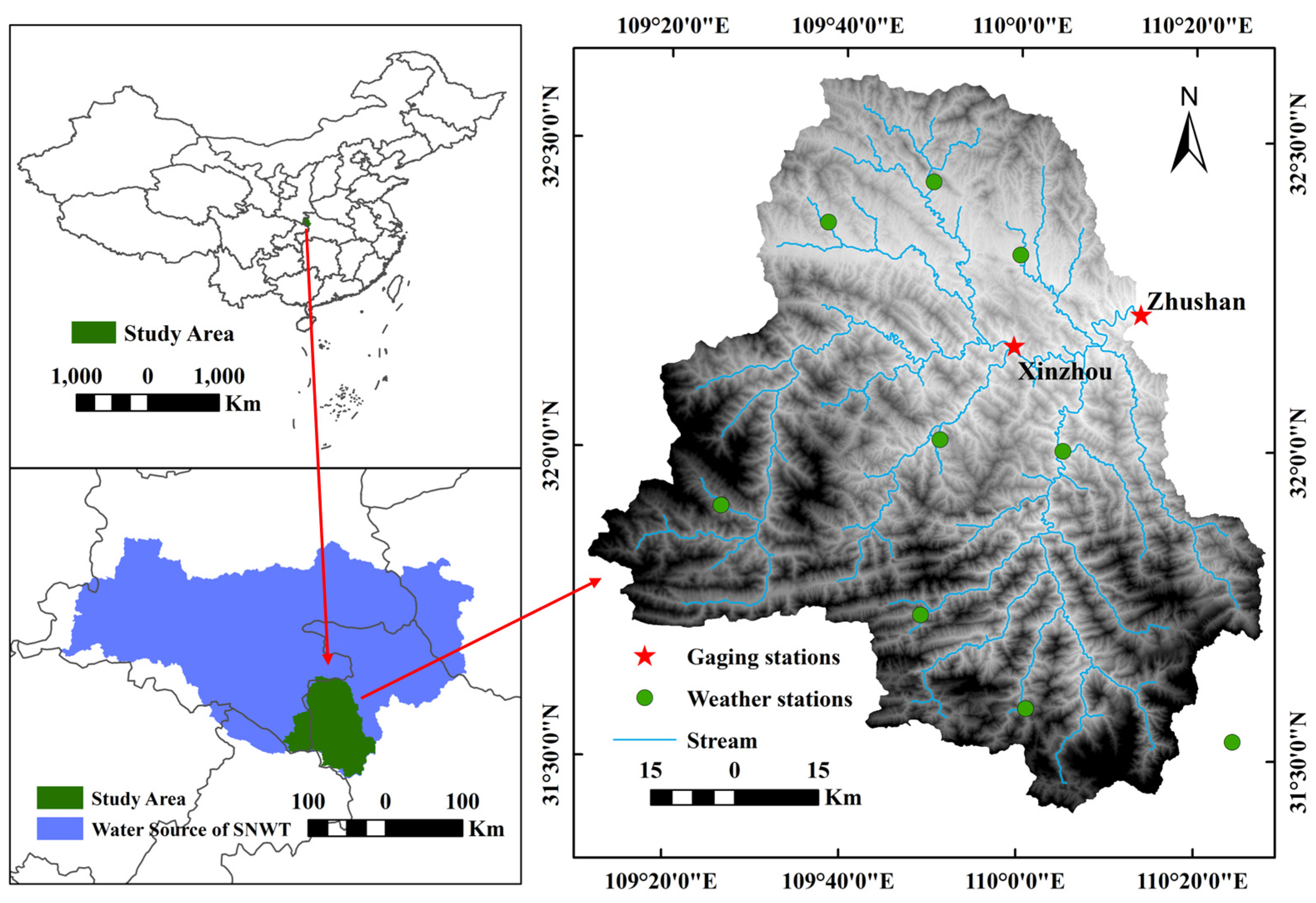
2.1. Study Area

The Upper Du Watershed is located in the DRA and lies between 31°25′ N and 32°48′ N and between 109°10′ E and 110°45′ E and covers an area of 8973 km² (Figure 1). Average annual temperature was 12.4 °C to 18.4 °C, and the average annual precipitation was 728 mm to 1480 mm over the past 50 years. The topography of the watershed is undulating and characterized by mountain ranges, steep slopes, and deep valleys. The elevation ranges from 220 m at the outlet of the Upper Du Watershed to 2833 m at the highest point in the watershed. The main soil types are yellow-brown soil (71.5%) and brown soil (18.5%), which correspond to Alfisols and Entisols, respectively, based on the USA Soil Taxonomy [20]. The main land use types are forest, shrubland, farmland, urban land and grassland. Most areas are covered by subtropical evergreen broad-leaved forest and mixed coniferous broad leaved forest. The main agricultural crops are corn and wheat.

2.2. Methods

2.2.1. Data Collection

In this study, we used daily streamflow data, daily meteorological data, digital elevation data, soil type information and four sets of land use data. Daily streamflow data (1965–2010) from two hydrological stations (Zhushan and Xinzhou) were obtained from the Hubei Provincial Water Resources Bureau. Daily meteorological data, which included daily precipitation; solar radiation; wind speed and direction; humidity; and maximum, minimum, and mean air temperature data from 1965 to 2010 were obtained from nine weather stations that were within or close to the watershed (Figure 1). Digital elevation data were obtained from the National Geomatics Center of China and are presented at a 25 m × 25 m spatial resolution. The soil type information was extracted from a soil type map (1:100,000) that was issued by the Soil Hubei Provincial Survey Office. Four sets of land use data (1978, 1987, 1999 and 2000) were obtained from the Changjiang River Water Resources Commission. Seven land use categories were identified: forest, farmland, urban land, grassland, shrub land, barren land, and water (Figure 2).

Figure 1. Location map and observation sites in the Upper Du Watershed. SNWT: South-to-North Water Transfer.

Figure 1. Location map and observation sites in the Upper Du Watershed. SNWT: South-to-North Water Transfer.

Figure 2. Land use maps of the Upper Du Watershed.

Figure 2. Land use maps of the Upper Du Watershed.

2.2.2. Baseflow Separation

The program “Bflow.exe” is a recursive digital filter used for baseflow separation that was first suggested by Lyne and Hollick [21]. It works on the premise that direct runoff and baseflow are the components of streamflow [22]. Streamflow data could be similarly partitioned by analyzing high- and low-frequency signals using a recursive filter technique [21]. Low-frequency signals are related to baseflow and high-frequency signals are related to direct runoff [23]. This technique is physically unrealistic but is objective, reproducible, and easily automated [18]. The equation of the filter is:

$$B{F}_t=\beta B{F}_{t-1}+\frac{1-\beta }{2}\left(Q_t+Q_{t-1}\right)$$

(1)

where BF is the baseflow, Q is the total streamflow, β is the filter parameter (0.925), and t is the time step [23]. Equation (1) is restricted with the condition that BF_t ≤ Q_t [1]. The BLOW program computes baseflow by filtering the streamflow data three times; i.e., 1-Pass, 2-Pass and 3-Pass after opening a DOS prompt window and switching to the directory that contains the streamflow and program data files. With every pass, there is a reduction in the baseflow as a percentage of the streamflow. The 1-Pass baseflow, which is consistent with manually estimated baseflow [22,23], was used in this study. The BFI (baseflow/streamflow) values generated with these parameters were similar to those reported by many studies in the nearby watersheds [12,24].

2.2.3. SWAT Model Setup

The SWAT model is able to assess the influence of land management methods on hydrological components in complicated watersheds that have various land cover areas, varying soils and different climate scenarios, by employing parameters with time step at daily scale [19]. Hydrology in small and large watersheds have been studied with numerous SWAT applications in many regions of the world [8,25]. The dynamics of the initiation of baseflow were studied with SWAT in detail. In addition, SWAT was used to simulate baseflow with deterministic equations and the spatial variability of baseflow processes were considered as well as the consequent changes in baseflow. This allowed the model to be used to support land use management [26]. Overall, the SWAT program is a suitable model for simulating baseflow considering various land use and management scenarios [27].

The SWAT model embedded within GIS requires the input of various spatial environmental data. First, based on the data, came from topography (from the DEM), soil, and land use maps, watershed areas were divided into 107 sub-watersheds and these were then further sub-divided into 674 hydrological response units. Second, watershed management information, the daily precipitation, insolation, wind speed and direction, humidity, and temperature data were input to improve the modeling accuracy. Third, the model calculated the baseflow data for each sub-watershed automatically based on all of the input data. The algorithmic equations for baseflow are:

$$Q_{b,i}=Q_{b,i-1}\cdot \exp (-\mathsf{\alpha }\cdot t)+W_i\cdot [1-\exp (-\mathsf{\alpha }\cdot t)]$$

(2)

where Q_b,i is the baseflow from the aquifer of watershed on day i (mm/day), α is the baseflow recession coefficient, and t is the time step. W_i indicates the recharge to the aquifer on the given day i (mm/day), which is calculated as follows:

$$W_i=[1-\exp (-\frac{1}{\delta })]\cdot W_{seep}+\exp (-\frac{1}{\delta })W_{i-1}$$

(3)

where δ is the delay time of the overlying geologic formations, and W_seep is the total amount of water exiting the bottom of the soil profile (mm/day) [28].

2.2.4. SWAT Calibration for Un-Gauged Sub-Watershed Baseflow

Digital filter-based programs have been widely used for model calibration because of the difficulties with measuring baseflow [29]. The daily data were aggregated to the monthly time scale for the model evaluation. In calibration of the model, the 1978 land use map and other spatial environmental data were input in the SWAT model. We calibrated the model parameters (Table 1) to make the watershed simulated (model-based) baseflow data from January 1971 to December 1980 correspond to the digital-based baseflow data in gauging stations with multiple runs. Based on the 1987 land use map, data from the Zhushan gauging station from January 1981 to December 1990 were used for validation. Based on the 1999 land use map, data for the subperiod from January 1991 to December 1990 from the Xinzhou gauging station were also used for the validation. The performance of the model was evaluated with E_NS, which ranged from −∞ to 1. Higher values indicated higher acceptable levels of performance. The range of R² from 0 to 1 indicated the degree of collinearity between the observed and simulated data. The average tendency of the simulated data to differ from the observed counterparts was measured with the percent bias (PBLAS) [30]. Low-magnitude values indicating accurate model simulation [30]. According to Moriasi [31], a model simulation is judged to be very good if E_NS > 0.75, R² > 0.75, and PBIAS = ±10. A similar approach was used by Nie [8].

Table 1. Parameters of the SWAT model used to calibrate baseflow in the Upper Du Watershed.

Parameter Database	Parameter	Definition	Optimal Value
.bsn	ESCO	Soil evaporation compensation factor	1
	EPCO	Plant water uptake compensation factor	1
	SURLAG	Surface runoff lag time	2
.GW	GW_DELAY	Delay days	10
	GW_REVAP	Re-evaporation coefficient	0.05
	ALPHA_BF	Baseflow alpha factor	0.5
.soil	SOL_AWC	Available soil water capacity	0.2
.sub	CH_N1	Manning’s “n” of tributary channels	0.1
.rte	CH_N2	Manning’s “n” of the main channel	0.02
.mgt	CN2	SCS curve number	39 (Forest)
			48 (Shrubland)
			68 (Grassland)
			81 (Farmland)
			89 (Urban)
			92 (Barren)
.GW	GWQMN	Threshold of return flow occurring in aquifer	0
	RCHRGDP	Deep aquifer percolation factor	0.05
.hru	SLSUBBSN	Slope length of the sub-basin	1.1
	HRU_SLP	Slope of Hydrological Response Unit (HRU)	0.1

SWAT: the Soil and Water Assessment Tool.

Table 1. Parameters of the SWAT model used to calibrate baseflow in the Upper Du Watershed.

Parameter Database	Parameter	Definition	Optimal Value
.bsn	ESCO	Soil evaporation compensation factor	1
	EPCO	Plant water uptake compensation factor	1
	SURLAG	Surface runoff lag time	2
.GW	GW_DELAY	Delay days	10
	GW_REVAP	Re-evaporation coefficient	0.05
	ALPHA_BF	Baseflow alpha factor	0.5
.soil	SOL_AWC	Available soil water capacity	0.2
.sub	CH_N1	Manning’s “n” of tributary channels	0.1
.rte	CH_N2	Manning’s “n” of the main channel	0.02
.mgt	CN2	SCS curve number	39 (Forest)
			48 (Shrubland)
			68 (Grassland)
			81 (Farmland)
			89 (Urban)
			92 (Barren)
.GW	GWQMN	Threshold of return flow occurring in aquifer	0
	RCHRGDP	Deep aquifer percolation factor	0.05
.hru	SLSUBBSN	Slope length of the sub-basin	1.1
	HRU_SLP	Slope of Hydrological Response Unit (HRU)	0.1

SWAT: the Soil and Water Assessment Tool.

2.2.5. Model Application

Land use maps from 1978 and 2007 were used in model calibration. The DEM and soil data was kept constant from January 1970 to December 2010. Only the land use maps are “changing”, while the other input data are “fixed”. Then, we obtained the data for the baseflow changes from the land use scenarios for 1978 to 2007 in the 107 sub-watersheds. We then extracted the data (area) on the changes in the individual land use types from the land use maps from 1978 to 2007 in the 107 sub-watersheds. The results were used to illustrate the baseflow change under the effects of land use changes in the watershed scale and to quantify the influences of land use changes on seasonal baseflow at the sub-watershed scale.

2.2.6. Statistical Analyses

To estimate the variables’ variability, the robust coefficient of variation (CV) was calculated as follows:

Rubost CV = 100% × normalized interquartile range (NIR)/median

(4)

where NIR is interquartile range multiplied by 0.7413 [32]. The PLS regression was used to determine the main watershed land use type that controls baseflow. For the analysis of the contribution of changes in influencing factors to baseflow at the sub-watershed scale, the following independent variables corresponded to changes in the seven land use types, barren, forest, shrubland, water, farmland, grassland, and urban, and the dependent variables corresponded to baseflow changes. In the PLS method, X is a matrix with n rows and p columns and Y is a matrix with n rows and q columns. Multivariate response variables are processed with the PLS method when Y is an n × q vector with q > 1. However, in this work, it was supposed that Y is a single variable, i.e., Y is n × 1 and X is n × p. To build a PLS model, X needs to be regressed onto the x-scores (T), which are used to predict the y-scores (U), which in turn are used to predict the responses Y. To avoid overfitting, the analyses searched for a set of components with the minimum value difference (cross-validated root mean squared error, RMSECV) between the explained variation in response (R²) and the predictive ability of the model (maximum cross-validated goodness of prediction, Q²). The regression coefficient indicates the direction of the relationship between each independent and dependent variable. Modeling of the PLS, which has several components, and calculating the Variable Influence on Projection (VIP) can indicate the importance of a predictor for variations. The information over all predictors and PLS dimensions was pooled with the VIP. The strength of influence for each predictor is indicated by the VIP values. The direction of the relationship between baseflow and the changes in land use types were described by the regression coefficients of the PLS models.

3. Results and Discussion

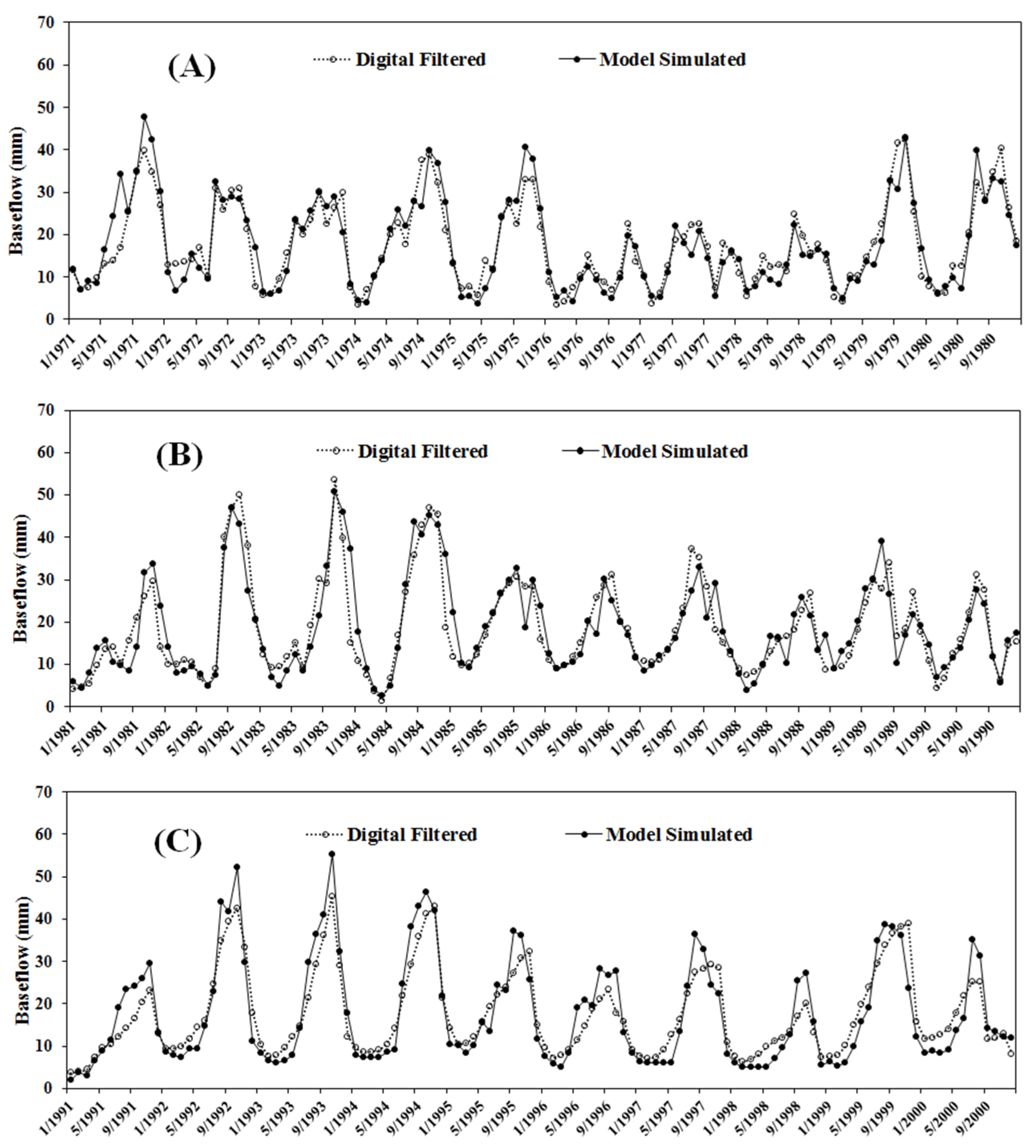
3.1. Un-Gauged Sub-Watersheds Baseflow

Figure 3 shows the monthly model-based and digital filter-based baseflow of the Upper Du Watershed during calibration and validation. The statistical performance was satisfactory according to the monthly E_NS, R², and PBIAS (Table 2). The statistical results showed good agreement by comparing the digital-based baseflow with the simulation, and the parameters calibrated for baseflow of the model could be used to simulate every sub-watershed. However, as shown in Figure 3, there was a difference between the filtered-based value and the simulated value. The filter-based value accounted for 34.3% of the annual flow volume and the model-based baseflow volume accounted for 35.0% of the annual flow volume. Most summers, the simulated value was overestimated, whereas it tended to be too low in winter. The depletion of a portion of the shallow aquifer storage of the watershed during the simulation accounted for the slight difference. The simulation revealed that there was seasonal storage fluctuation and equilibrium was maintained for the deep aquifer. Rapid percolation of rainfall occurs during the summer, and the shallow aquifer, which is the important resource for baseflow, quickly receives recharge from the unsaturated soil profile percolation; in winter, the underground storage is released more slowly [29].

Table 2. Examination of the performance of SWAT in the Upper Du Watershed.

Stations	Period	ENS a	PBIAS b	R2	Rating
Zhushan	Calibration (1971–1980)	0.83	3.9	0.85	Very good c
	Validation (1981–1990)	0.80	4.5	0.81	Very good
	Overall (1971–1990)	0.82	4.2	0.83	Very good
Xinzhou	Validation (1991–2000)	0.77	1.5	0.87	Very good
	Overall (1991–2010)	0.77	1.5	0.87	Very good

^a Sampling E_NS = Nash-Sutcliffe efficiency; ^b Sampling PBIAS = Percent Bias; ^c The performance of the SWAT model is very good when E_NS > 0.75 and PBIAS values are in the range of ±10%.

Table 2. Examination of the performance of SWAT in the Upper Du Watershed.

Stations	Period	ENS a	PBIAS b	R2	Rating
Zhushan	Calibration (1971–1980)	0.83	3.9	0.85	Very good c
	Validation (1981–1990)	0.80	4.5	0.81	Very good
	Overall (1971–1990)	0.82	4.2	0.83	Very good
Xinzhou	Validation (1991–2000)	0.77	1.5	0.87	Very good
	Overall (1991–2010)	0.77	1.5	0.87	Very good

^a Sampling E_NS = Nash-Sutcliffe efficiency; ^b Sampling PBIAS = Percent Bias; ^c The performance of the SWAT model is very good when E_NS > 0.75 and PBIAS values are in the range of ±10%.

Figure 3. Monthly digital filtered-based and model-based baseflow in the Upper Du Watershed for the calibration (from 1 January 1971 to 31 December 1980) at Zhushan station (A); validation (from 1 January 1981 to 31 December 1990) at Zhushan station (B); and validation (from 1 January 1991 to 31 December 2000) in Xinzhou station (C).

Figure 3. Monthly digital filtered-based and model-based baseflow in the Upper Du Watershed for the calibration (from 1 January 1971 to 31 December 1980) at Zhushan station (A); validation (from 1 January 1981 to 31 December 1990) at Zhushan station (B); and validation (from 1 January 1991 to 31 December 2000) in Xinzhou station (C).

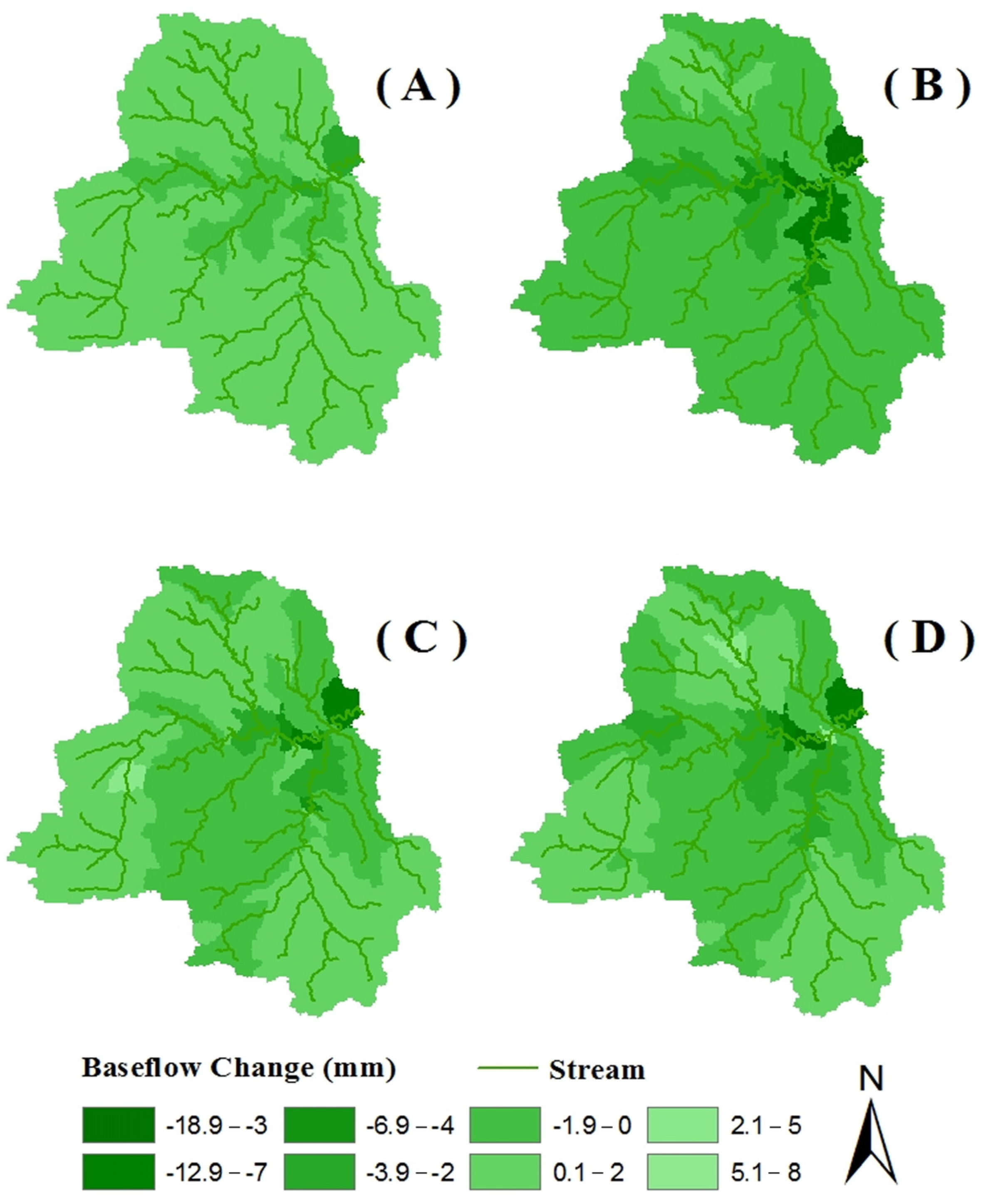
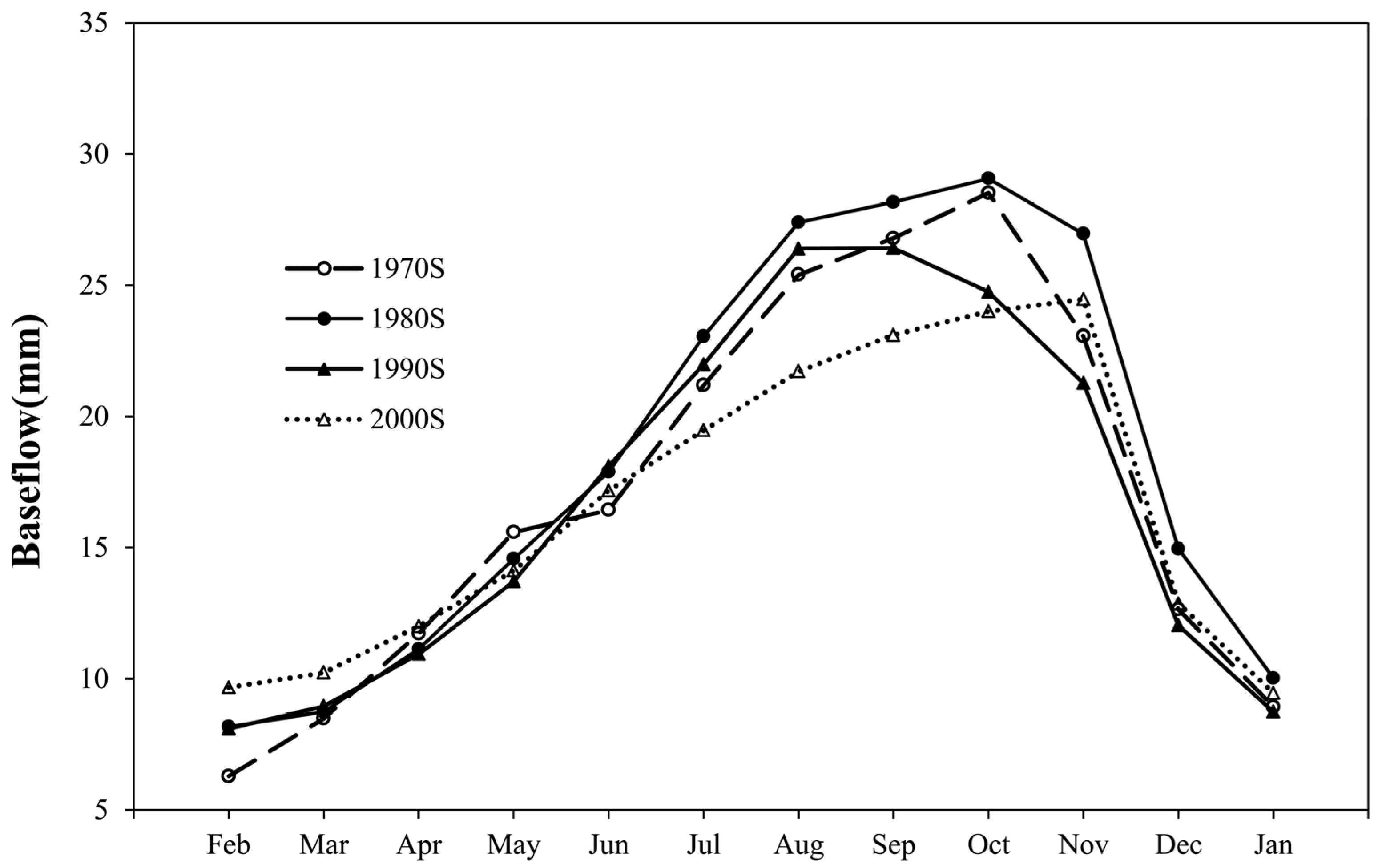
3.2. Temporal and Spatial Distribution of Baseflow

Figure 4 shows the changes in the timing of digital-based baseflow. The average annual baseflow over the entire watershed for four study periods (1970s, 1980s, 1990s, and 2000s) was 205.0, 220.1, 201.3, and 198.2 mm, respectively. The mean monthly baseflow showed a prominent increased in spring, which might have been affected by the rainfall increase (3 mm) from the 1970s to the 2000s in this season. The prominent late-autumn peaks were likely to diminish and a larger proportion of discharge shifted to early winter. The processes causing the temporal changes in baseflow also resulted in spatial changes. Figure 5 shows the model-based baseflow changes between 1978 and 2007 at the sub-watershed scale and Table 3 shows that the seasonal baseflow in the 107 sub-watersheds varied substantially according to CV. The spatial distribution of the baseflow changes of this watershed can be broadly divided into two parts: the area near the major stream channels mainly covered by farmland and urban areas, and the more distant area that is mainly covered by forest. The baseflow change during February, March, and April (spring) of 2007 was not substantially different from the conditions during 1978 for much of the Upper Du Watershed (Figure 5A), as the increase was inconspicuous (less than 2 mm). The decrease in baseflow was less than 3.9 mm in the area along the major stream channels. Simulations indicated that the baseflow during May, June, and July (summer) of 2007 declined (0.1–1.9 mm) throughout the area, which was mainly covered by forest, relative to 1978. Larger decreases in baseflow, ranging from 2.0 to 18.9 mm, were simulated in the area mainly covered by farmland and urban land use near the main stream channel in the middle and northern parts of the watershed. The baseflow decreased during August, September, and October (autumn) in the middle and northern parts of the watershed in 2007. The baseflows in the northern, southwestern, and southeastern portions distant from the major stream network of the watershed showed a slight increase, whereas they showed a slight decrease in the summer months and were not markedly different volumetrically from the historic period. Patterns of baseflow changes in November, October, and January (winter) were similar to those in the autumn months; however, the baseflow recession expanded to areas distant from the major stream network.

Figure 4. Watershed-scale average monthly baseflow for the 1970s, 1980s, 1990s, and 2000s.

Figure 4. Watershed-scale average monthly baseflow for the 1970s, 1980s, 1990s, and 2000s.

Figure 5. Changes in baseflow from 1970s to 2000s calculated for spring (A); summer (B); autumn (C); and winter (D) seasons.

Figure 5. Changes in baseflow from 1970s to 2000s calculated for spring (A); summer (B); autumn (C); and winter (D) seasons.

Table 3. Robust coefficient of variation (CV) for the average monthly baseflow of each sub-watershed in this study.

Seasonal Baseflow	Land Use Scenarios	Robust Coefficient of Variation
Spring baseflow	1978	216.8%
	2007	239.2%
Summer baseflow	1978	241.5%
	2007	260.4%
Autumn baseflow	1978	232.8%
	2007	234.5%
Winter baseflow	1978	219.3%
	2007	226.3%

Table 3. Robust coefficient of variation (CV) for the average monthly baseflow of each sub-watershed in this study.

Seasonal Baseflow	Land Use Scenarios	Robust Coefficient of Variation
Spring baseflow	1978	216.8%
	2007	239.2%
Summer baseflow	1978	241.5%
	2007	260.4%
Autumn baseflow	1978	232.8%
	2007	234.5%
Winter baseflow	1978	219.3%
	2007	226.3%

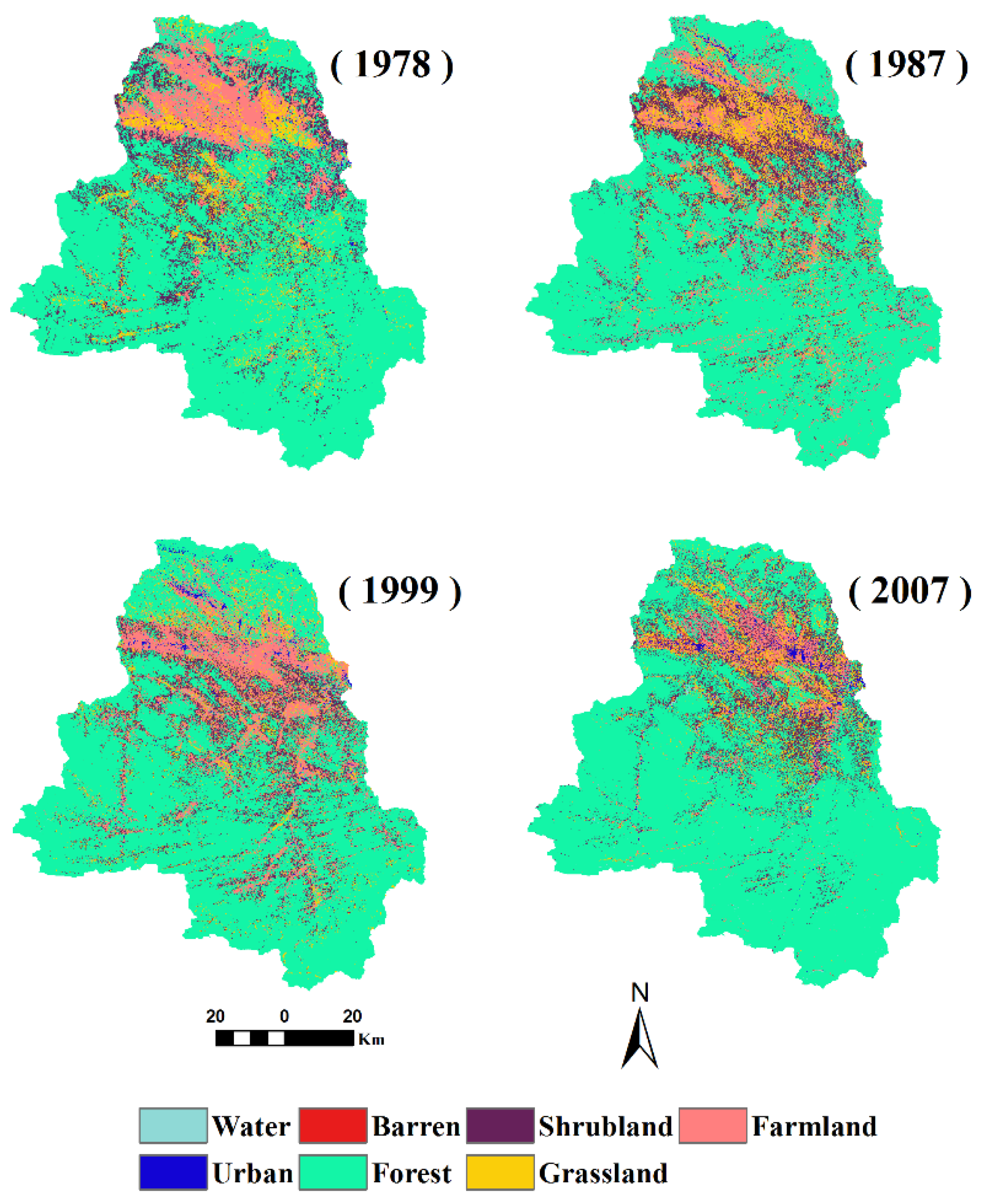
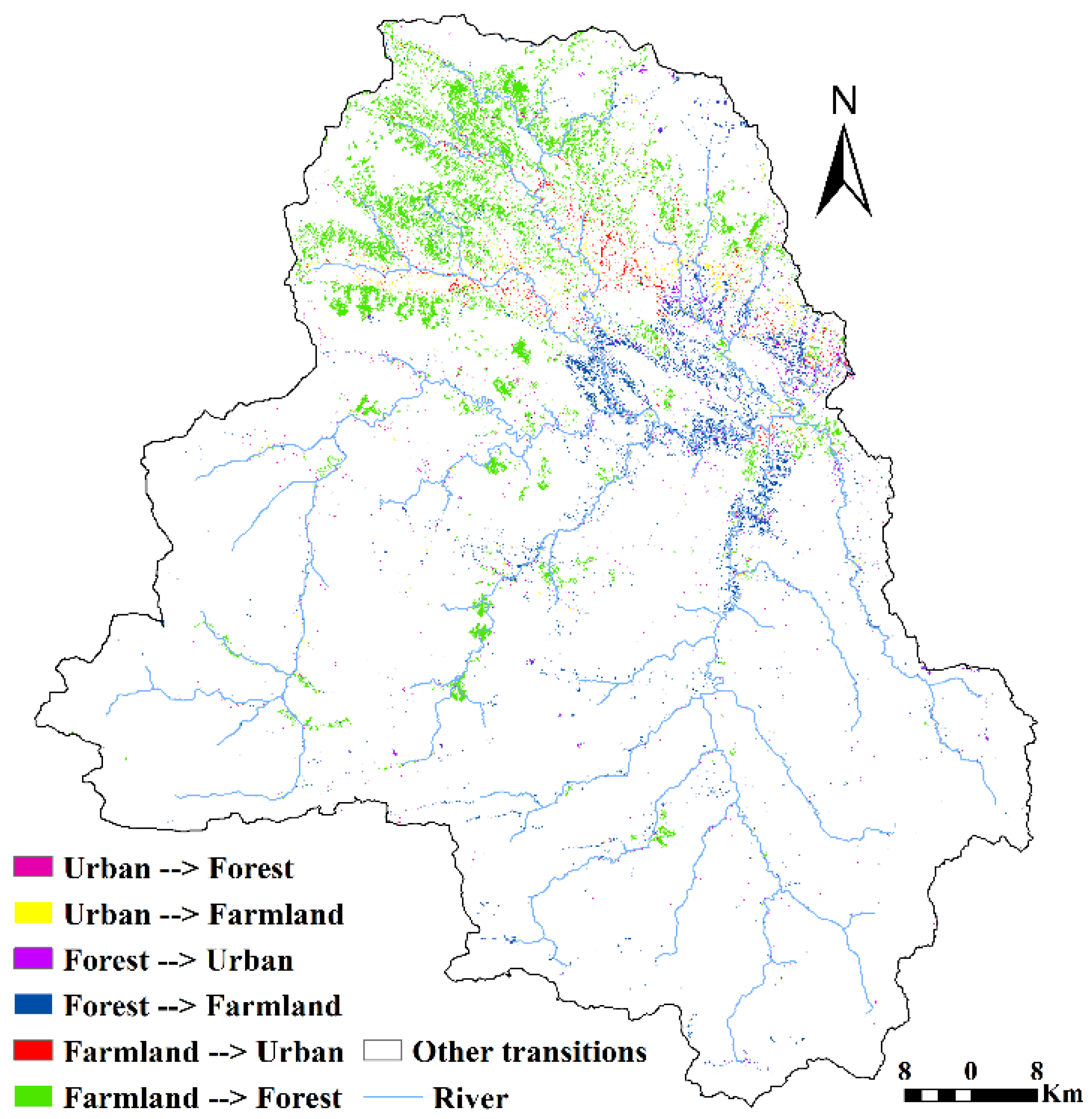
3.3. Influences of Forest and Other Land Use Changes on Baseflow

The land use changes during the four periods are given in Table 4. Comparing the land cover maps for 1978 and 1999, the area corresponding to forest decreased from 6365.5 km² to 6232.1 km² with an annual reduction of 6.1 km², whereas the area corresponding to farmland increased by 15.2 km² per year. However, after 1999, rapid forest expansion and urban development occurred in this region. The most remarkable land use variations are the increase in forest of 76.1 km² per year and the decline in farmland by 86.9 km² per year. These dynamics were associated with government policy. In 1978, “Household Responsibility System” was initiated by the central government, and most areas of China entered into the period of cultivation [33]. In 1999, Grain for Green (GFG) was implemented and directly engaged millions of farmers in protecting certain areas, thus, China entered into the period of ecological restoration [34].

Table 4. Percent of land use areas and changes in the Upper Du Watershed (1978–2007).

Land Use (%)	1978	1987	1999	2007	1978–1987	1987–1999	1999–2007	1978–2007
Forest	70.9	70.4	69.3	76.2	−0.5	−1.1	+6.9	+5.3
Farmland	9.8	10.2	13.6	5.8	+0.4	+3.4	−7.8	−4.0
Urban	0.8	0.9	1.1	1.4	+0.1	+0.2	+0.4	+0.6
Grassland	7.6	7.3	5.9	6.1	−0.3	−1.4	+0.2	−1.5
Shrubland	10.2	10.4	9.4	9.5	−0.2	+1.0	−0.1	−0.7
Barren	0.3	0.4	0.4	0.7	+0.1	0	+0.3	+0.4
Water	0.4	0.4	0.3	0.3	0	−0.1	0	−0.1

Table 4. Percent of land use areas and changes in the Upper Du Watershed (1978–2007).

Land Use (%)	1978	1987	1999	2007	1978–1987	1987–1999	1999–2007	1978–2007
Forest	70.9	70.4	69.3	76.2	−0.5	−1.1	+6.9	+5.3
Farmland	9.8	10.2	13.6	5.8	+0.4	+3.4	−7.8	−4.0
Urban	0.8	0.9	1.1	1.4	+0.1	+0.2	+0.4	+0.6
Grassland	7.6	7.3	5.9	6.1	−0.3	−1.4	+0.2	−1.5
Shrubland	10.2	10.4	9.4	9.5	−0.2	+1.0	−0.1	−0.7
Barren	0.3	0.4	0.4	0.7	+0.1	0	+0.3	+0.4
Water	0.4	0.4	0.3	0.3	0	−0.1	0	−0.1

Table 5 shows statistics of individual land use changes at the sub-watershed scale. The CV values indicated that the land use types varied substantially in the 107 sub-watersheds, except the water. This phenomenon was caused by the non-uniform distribution of forests and changes in farmland. First, before 1999, diminishing forests are linked with the efficiency of deforestation, which was affected by the physical accessibility of the forest stand, as exemplified through such metrics as the linear distances to highways, roads, and navigable rivers [35]. Second, expanded farmland associated with cultivation mainly occurred in land near stream channels over the entire watershed. Finally, after 1999, the land use distribution at the sub-watersheds scale became more irregular because only specific farmland (normally with slopes >25°) was transformed into forests [36].

Land use transformation maps were produced based on the intersecting of the 1978 and 2007 land use maps (Figure 6). Since the land use maps have six land use types, the land use transformations can have a maximum of 36 classes. However, many transformations were not evident in the maps. In this study, only forest/farmland/urban transformations were considered. The farmland and urban expansion mainly development in the lower stretches and middle of the northern area of the watershed, largely matching the decreases in baseflow. Baseflow change during the spring of 2007 was only slightly different from the conditions during 1978 throughout most of the watershed with a change of less than 2 mm over most of the watershed away from the main stream network, which is mainly covered by forest. This is because spring is the initial growing season for trees and ET is much lower than in other growing seasons [37]. In summer, the majority of the farmland converted to forest and there was high seasonal evapotranspiration in the sub-watersheds and this spatially corresponded with the decrease in baseflow in the northern, southwestern and southeastern portions of the watershed.

Table 5. Robust Coefficient of Variation for the land use types of each sub-watershed in Upper Du Watershed.

Land Use Maps	Land Use Types	Robust Coefficient of Variation
1978	Forest	159.6%
	Farmland	350.0%
	Urban	304.0%
	Grassland	159.8%
	Shrubland	223.1%
	Barren	197.9%
	Water	279.8%
2007	Forest	193.7%
	Farmland	394.8%
	Urban	352.9%
	Grassland	396.7%
	Shrubland	203.5%
	Barren	514.1%
	Water	213.3%

Table 5. Robust Coefficient of Variation for the land use types of each sub-watershed in Upper Du Watershed.

Land Use Maps	Land Use Types	Robust Coefficient of Variation
1978	Forest	159.6%
	Farmland	350.0%
	Urban	304.0%
	Grassland	159.8%
	Shrubland	223.1%
	Barren	197.9%
	Water	279.8%
2007	Forest	193.7%
	Farmland	394.8%
	Urban	352.9%
	Grassland	396.7%
	Shrubland	203.5%
	Barren	514.1%
	Water	213.3%

Figure 6. Land use transformation maps of the Upper Du Watershed from 1978 to 2007.

Figure 6. Land use transformation maps of the Upper Du Watershed from 1978 to 2007.

In autumn and winter, simulations indicated a general increase in the baseflow of 0.1–2.0 mm in 2007 compared to 1978 over much of northern, southwestern and southeastern portions of the watershed. This change in baseflow was due to the large effects of forests in this area far from the stream network as well as the low ET during later growing and non-growing seasons. A larger proportion of baseflow recharge occurred in these seasons. Evapotranspiration diminished the baseflow recharge pulse from May to January, and the comparison of variations of baseflow and changes in land use types suggests a strong negative relationship between baseflow and the forest and farmland in these three seasons (average R² is 0.83 and 0.79, respectively).

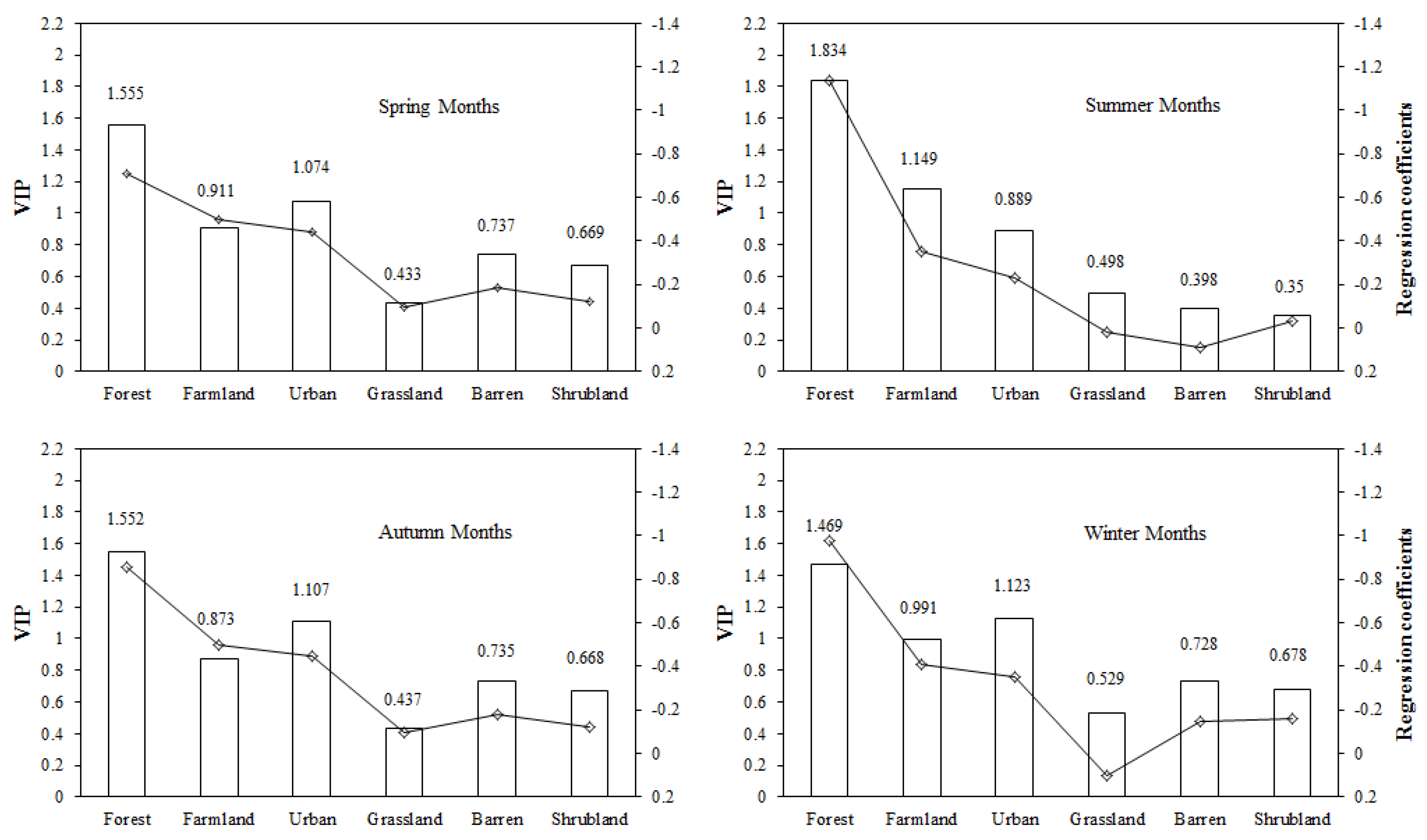
3.4. Contribution of Land Use Changes to Baseflow

Table 6 provided the summaries of the PLS model constructed for the four seasons. For the spring, autumn, and winter models, the first component explains 74.7%, 74.4%, and 69.1% of the variation in baseflow, respectively. The addition of the second component explained, respectively, 79.1%, 78.8%, and 71.3% of the variation and generated a minimum RMSECV. The addition of components to the PLS led to higher RMSECV values (Table 6). For these models, two predictor variables, namely, forest and urban land, had VIP scores greater than 1, followed by farmland, shrubland, grassland, and barren land with VIP scores less than 1 (ranges from 0.991 to 0.433). Forest also had larger negative regression coefficients (−0.708, −0.854, and −1.108) (Figure 7).

Figure 7. Regression coefficients (lines) and the Variable Influence on Projection (VIP) (bars) of each land use type.

Figure 7. Regression coefficients (lines) and the Variable Influence on Projection (VIP) (bars) of each land use type.

Table 6. Summary of partial least-squares (PLS) regression models of baseflow for all sub-watersheds.

Response Y	R2 a	Q2 b	Component	% of Explained Variability in Y	Cumulative Explained in Y (%)	RMSECV c	Q2cum d
Spring baseflow	0.79	0.67	1	74.7	74.7	0.88	0.634
			2	4.4	79.1	0.80	0.666
			3	0.4	79.5	0.81	0.656
Summer baseflow	0.82	0.72	1	71.8	71.8	6.09	0.658
			2	9.8	81.6	5.12	0.718
			3	1.2	82.8	5.70	0.709
Autumn baseflow	0.79	0.68	1	74.4	74.4	0.88	0.644
			2	4.4	78.8	0.80	0.682
			3	0.4	79.2	0.81	0.667
Winter baseflow	0.71	0.55	1	69.1	69.1	1.29	0.597
			2	2.2	71.3	1.26	0.547
			3	0.1	71.4	1.27	0.494

^a Sampling R² = goodness of fit; ^b Q² = maximum cross-validated goodness of prediction; ^c RMSECV = cross-validated root mean squared error; and ^d Q²_cum = cumulative cross-validated goodness of prediction.

Table 6. Summary of partial least-squares (PLS) regression models of baseflow for all sub-watersheds.

Response Y	R2 a	Q2 b	Component	% of Explained Variability in Y	Cumulative Explained in Y (%)	RMSECV c	Q2cum d
Spring baseflow	0.79	0.67	1	74.7	74.7	0.88	0.634
			2	4.4	79.1	0.80	0.666
			3	0.4	79.5	0.81	0.656
Summer baseflow	0.82	0.72	1	71.8	71.8	6.09	0.658
			2	9.8	81.6	5.12	0.718
			3	1.2	82.8	5.70	0.709
Autumn baseflow	0.79	0.68	1	74.4	74.4	0.88	0.644
			2	4.4	78.8	0.80	0.682
			3	0.4	79.2	0.81	0.667
Winter baseflow	0.71	0.55	1	69.1	69.1	1.29	0.597
			2	2.2	71.3	1.26	0.547
			3	0.1	71.4	1.27	0.494

^a Sampling R² = goodness of fit; ^b Q² = maximum cross-validated goodness of prediction; ^c RMSECV = cross-validated root mean squared error; and ^d Q²_cum = cumulative cross-validated goodness of prediction.

In the summer model, the first component was dominated by forest and farmland and explained 71.8% of the variance in the dataset regarding changes in baseflow (Table 6). The second component was dominated by farmland and urban areas and addition of this component explained 81.6% of the total variance. Adding more components to the PLS models failed to substantially improve the explained variance (Table 6). The lower importance of some variance predictors in a particular component was indicated by the distance of the PLS weights from the original variables. Also, a more convenient and comprehensive expression of the relative importance of predictors can be derived from exploring their VIP values [38]. As shown in Figure 7, two predictor variables, namely forest and farmland, had VIP scores greater than 1 (1.834 and 1.149, respectively) and regression coefficients of −1.135 and −0.350, respectively, followed by the percentage of urban (VIP = 0.889; coefficient = −0.231), grassland (VIP = 0.498; coefficient = 0.020), and barren land (VIP = 0.398; coefficient = 0.091). Hence, these variables are used in the prediction model to obtain projected predictands. The negative regression coefficient of forestland was due to the greater interception of the canopy and ET rates (trees transfer subsurface water to leaves and then to the atmosphere) [39]. According to Price [3], the baseflow response to farmland may be positivity or negativity associated with the crop irrigation practices, natural losses via ET, and variable infiltration. Our results suggest that the negative relationships between farmland and baseflow in the Upper Du Watershed may be correlated with crops, which are irrigated from surface water storage associated with the stream network, and the great ET loss of crops, which is agreed with the conclusions of many researchers [9,40]. Following urbanization, throughfall decreases in building zones where rainfall interception occurs; additionally, infiltration is reduced by soil compaction and impervious surface additions, and water flushes more quickly through the watershed as a result of decreases in the hydraulic resistance of land surfaces and channels [3,41,42].

The effects of forested areas are greater than that of agricultural areas. This phenomenon can be explained as follows. First, baseflow regression associated with ET in a watershed with perennial vegetation (e.g., trees) is generally higher than crops (i.e., farmland) [37,39]. Second, the transpiration of perennial forest vegetation influences the baseflow regression throughout the whole growing season, whereas the transpiration of seasonal crops influences the baseflow regression only during the mid-growing and late-growing seasons [9]. Overall, the strong baseflow regression of forests is sustained for a longer time. Thus, we can suggest that the baseflow will increase with the replacement of forest by farmland. These results are consistent with Sun [43] pertaining to a study on the water yield response to forest management. The effects of forested areas are greater than that of urban land due to the increase of non-contributing impervious surfaces in urban areas, which mitigate the negative influences of urbanization on baseflow [44]. The impacts of urbanization are characterized by the total area of impervious surfaces in a watershed [45]. The total impervious area can be divided into the effective impervious area and the non-contributing impervious area (such as pervious areas and leaky water infrastructure) [45,46]. However, considering only the effective impervious area of a watershed is not sufficient [44]. Non-contributing impervious areas, which are formally addressed through effective impervious areas [47], increase with increases in urban land. Thus, baseflow maybe increase when forestland changes to urban. Similar conclusions were reported by Boggs and Sun [48].

4. Conclusions

Our study quantifies the relative importance of the land use types on baseflow at the sub-watershed scale. The results indicate that the dynamics of baseflow are closely associated with changes of land use. The major negative factors that affect baseflow were found to be changes to forest, followed by farmland and urban land. Grassland, barren land, and shrubland did not result in a significant impact on baseflow in our study watershed.

This study could be applied to many types of watersheds if the time series data and special land use information are available, and thereby provides useful quantitative information on internal dynamics of baseflow and major drivers in watersheds for forest and watershed management. From a forest landscape ecology perspective, a watershed’s land cover patterns might be important for determining hydrological processes. Therefore, future research should focus on the influence of forestland cover patterns on baseflow changes.

References

1. Eckhardt, K. A comparison of baseflow indices, which were calculated with seven different baseflow separation methods. J. Hydrol. 2008, 352, 168–173. [Google Scholar] [CrossRef]
2. Smakhtin, V.U. Low flow hydrology: A review. J. Hydrol. 2001, 240, 147–186. [Google Scholar] [CrossRef]
3. Price, K. Effects of watershed topography, soils, land use, and climate on baseflow hydrology in humid regions: A review. Prog. Phys. Geogr. 2011, 35, 465–492. [Google Scholar] [CrossRef]
4. Knox, J.C. Floodplain sedimentation in the Upper Mississippi Valley: Natural versus human accelerated. Geomorphology 2006, 79, 286–310. [Google Scholar] [CrossRef]
5. Varis, O.; Vakkilainen, P. China’s 8 challenges to water resources management in the first quarter of the 21st Century. Geomorphology 2001, 41, 93–104. [Google Scholar] [CrossRef]
6. Zhuang, D.F.; Deng, X.Z.; Zhan, J.Y.; Zhao, T. A study on the spatial distribution of land use change in Beijing. Geogr. Res. 2002, 21, 667–674. (In Chinese) [Google Scholar]
7. Dou, X.; Chen, B.; Black, T.A.; Jassal, R.S.; Che, M. Impact of nitrogen fertilization on forest carbon sequestration and water loss in a chronosequence of three Douglas-fir stands in the pacific northwest. Forests 2015, 6, 1897–1921. [Google Scholar] [CrossRef]
8. Nie, W.M.; Yuan, Y.P.; Kepner, W.; Nash, M.S.; Jackson, M.; Erickson, C. Assessing impacts of land use changes on hydrology for the upper San Pedro watershed. J. Hydrol. 2011, 407, 105–114. [Google Scholar] [CrossRef]
9. Zhang, Y.K.; Schilling, K.E. Increasing streamflow and baseflow in Mississippi River since the 1940s: Effect of land use change. J. Hydrol. 2006, 324, 412–422. [Google Scholar] [CrossRef]
10. Ma, X.; Xu, J.C.; Luo, Y.; Aggarwal, S.P.; Li, J.T. Response of hydrological processes to land-cover and climate changes in Kejie watershed, south-west China. Hydrol. Process. 2009, 23, 1179–1191. [Google Scholar] [CrossRef]
11. Artita, K.S.; Kaini, P.; Nicklow, J.W. Examining the possibilities: Generating alternative watershed-scale BMP designs with evolutionary algorithms. Water Resour. Manag. 2013, 27, 3849–3863. [Google Scholar] [CrossRef]
12. Zhou, F.; Xu, Y.; Chen, Y.; Xu, C.Y.; Gao, Y.; Du, J. Hydrological response to urbanization at different spatio-temporal scales simulated by coupling of CLUE-S and the SWAT model in the Yangtze River Delta region. J. Hydrol. 2013, 485, 113–125. [Google Scholar] [CrossRef]
13. Luedeling, E.; Gassner, A. Partial least squares regression for analyzing walnut phenology in California. Agric. For. Meteorol. 2012, 158, 43–52. [Google Scholar] [CrossRef]
14. Shi, Z.H.; Ai, L.; Li, X.; Huang, X.D.; Wu, G.L.; Liao, W. Partial least-squares regression for linking land-cover patterns to soil erosion and sediment yield in watersheds. J. Hydrol. 2013, 498, 165–176. [Google Scholar] [CrossRef]
15. Abdi, H.; Williams, L.J. Principal component analysis. Wiley Interdiscip. Rev. Comput. Stat. 2010, 2, 433–459. [Google Scholar] [CrossRef]
16. Geladi, P.; Sethson, B.; Nyström, J.; Lillhonga, T.; Lestander, T.; Burger, J. Chemometrics in spectroscopy. Spectrochim. Acta B At. Spectrosc. 2004, 59, 1347–1357. [Google Scholar] [CrossRef]
17. Li, L.; Shi, Z.; Yin, W.; Zhu, D.; Ng, S.L.; Cai, C.; Lei, A. A fuzzy analytic hierarchy process (FAHP) approach to eco-environmental vulnerability assessment for the Danjiangkou Reservoir Area, China. Ecol. Model. 2009, 220, 3439–3447. [Google Scholar] [CrossRef]
18. Wang, J.; Huang, B.; Fu, D.; Atkinson, P.M. Spatiotemporal variation in surface urban heat island intensity and associated determinants across major Chinese cities. Remote Sens. 2015, 7, 3670–3689. [Google Scholar] [CrossRef]
19. Yan, B.; Fang, N.F.; Zhang, P.C.; Shi, Z.H. Impacts of land use change on watershed streamflow and sediment yield: An assessment using hydrologic modelling and partial least squares regression. J. Hydrol. 2013, 484, 26–37. [Google Scholar] [CrossRef]
20. Soil Survey Staff. Soil Taxonomy, A Basic System of Soil Classification for Making and Interpreting Soil Surveys, 2nd ed.Agriculture Handbook No. 436; USDA Natural Resources Conservation Service, U.S. Government Printing 23 Office: Washington, DC, USA, 1999; pp. 160–162, 494–495.
21. Lyne, V.; Hollick, M. Stochastic time-variable rainfall-runoff modelling. Canberra 1979, 79, 89–93. [Google Scholar]
22. Arnold, J.G.; Allen, P.M. Automated methods for estimating baseflow and ground water recharge from streamflow records. J. Am. Water Resour. Assoc. 1999, 35, 411–424. [Google Scholar] [CrossRef]
23. Ahiablame, L.; Chaubey, I.; Engel, B.; Cherkauer, K.; Merwade, V. Estimation of annual baseflow at ungauged sites in Indiana USA. J. Hydrol. 2013, 476, 13–27. [Google Scholar] [CrossRef]
24. Fang, N.F.; Shi, Z.H.; Li, L.; Guo, Z.L.; Liu, Q.J.; Ai, L. The effects of rainfall regimes and land use changes on runoff and soil loss in a small moutainous watershed. Catena 2012, 99, 1–8. [Google Scholar] [CrossRef]
25. Shi, Z.H.; Huang, X.D.; Ai, L.; Fang, N.F.; Wu, G.L. Quantitative analysis of factors controlling sediment yield in mountainous watersheds. Geomorphology 2014, 226, 193–201. [Google Scholar] [CrossRef]
26. Salerno, F.; Tartari, G. A coupled approach of surface hydrological modelling and Wavelet Analysis for understanding the baseflow components of river discharge in karst environments. J. Hydrol. 2009, 376, 295–306. [Google Scholar] [CrossRef]
27. Kushwaha, A.; Jain, M.K. Hydrological simulation in a forest dominated watershed in Himalayan region using SWAT model. Water Resour. Manag. 2013, 27, 3005–3023. [Google Scholar] [CrossRef]
28. Neitsch, S.L.; Arnold, J.G.; Kiniry, J.R.; Williams, J.R.; King, K.W. Soil Water Assessment Tool Theoretical Document, Version 2000, Grassland, Soil and Water Research Laboratory. Available online: http://www.brc.tamus.edu/swat/doc.html (accessed on 7 May 2012).
29. Luo, Y.; Arnold, J.; Allen, P.; Chen, X. Baseflow simulation using SWAT model in an inland river basin in Tianshan Mountains, Northwest China. Hydrol. Earth Syst. Sci. 2012, 16, 1259–1267. [Google Scholar] [CrossRef]
30. Gupta, H.V.; Sorooshian, S.; Yapo, P.O. Status of automatic calibration for hydrologic models: Comparison with multilevel expert calibration. J. Hydrol. Eng. 1999, 4, 135–143. [Google Scholar] [CrossRef]
31. Moriasi, D.N.; Arnold, J.G.; van Liew, M.W.; Bingner, R.L.; Harmel, R.D.; Veith, T.L. Model evaluation guidelines for systematic quantification of accuracy in watershed simulations. Trans. ASABE 2007, 50, 885–900. [Google Scholar] [CrossRef]
32. Temnerud, J.; Düker, A.; Karlsson, S.; Allard, B.; Köhler, S.; Bishop, K. Landscape scale patterns in the character of natural organic matter in a Swedish boreal stream network. Hydrol. Earth Syst. Sci. 2009, 13, 1567–1582. [Google Scholar] [CrossRef]
33. Li, X.B. Change of cultivated land area in china during the past 20 years and its policy implications. J. Nat. Resour. 1999, 14, 329–333. (In Chinese) [Google Scholar]
34. Lü, Y.H.; Fu, B.J.; Feng, X.M.; Zeng, Y.; Liu, Y.; Chang, R.Y.; Sun, G.; Wu, B.F. A policy-driven large scale ecological restoration: Quantifying ecosystem services changes in the Loess Plateau of China. PLoS ONE 2012, 7, e31782. [Google Scholar] [CrossRef] [PubMed]
35. Laurance, W.F.; Albernaz, A.K.M.; Schroth, G.; Fearnside, P.M.; Bergen, S.; Venticinque, E.M.; da Costa, C. Predictors of deforestation in the Brazilian Amazon. J. Biogeogr. 2002, 29, 737–748. [Google Scholar] [CrossRef]
36. Gao, Z.L.; Fu, Y.L.; Li, Y.H.; Liu, J.X.; Chen, N.; Zhang, X.P. Trends of streamflow, sediment load and their dynamic relation for the catchments in the middle reaches of the Yellow River over the past five decades. Hydrol. Earth Syst. Sci. 2012, 16, 3219–3231. [Google Scholar] [CrossRef]
37. FAO (Food and Agriculture Organization of the United Nations). Crop Evapotranspiration, Guidelines for Computing Crop Water Requirements; FAO Irrigation and Drainage Paper 56; Food and Agriculture Organization of the United Nations: Rome, Italy, 1998. [Google Scholar]
38. Onderka, M.; Wrede, S.; Rodný, M.; Pfister, L.; Hoffmann, L.; Krein, A. Hydrogeologic and landscape controls of dissolved inorganic nitrogen (DIN) and dissolved silica (DSi) fluxes in heterogeneous catchments. J. Hydrol. 2012, 450, 36–47. [Google Scholar] [CrossRef]
39. Wittenberg, H. Effects of season and man-made changes on baseflow and flow recession: Case studies. Hydrol. Process. 2003, 17, 2113–2123. [Google Scholar] [CrossRef]
40. Juckem, P.F.; Hunt, R.J.; Anderson, M.P.; Robertson, D.M. Effects of climate and land management change on streamflow in the driftless area of Wisconsin. J. Hydrol. 2008, 355, 123–130. [Google Scholar] [CrossRef]
41. Burns, D.; Vitvar, T.; McDonnell, J.; Hassett, J.; Duncan, J.; Kendall, C. Effects of suburban development on runoff generation in the Croton River Basin, New York, USA. J. Hydrol. 2005, 311, 266–281. [Google Scholar] [CrossRef]
42. Woltemade, C.J. Impact of residential soil disturbance on infiltration rate and stormwater runoff. J. Am. Water Resour. Assoc. 2010, 46, 700–711. [Google Scholar] [CrossRef]
43. Sun, G.; Zhou, G.; Zhang, Z.; Wei, X.; McNulty, S.G.; Vose, J.M. Potential water yield reduction due to forestation across China. J. Hydrol. 2006, 328, 548–558. [Google Scholar] [CrossRef]
44. Hamel, P.; Daly, E.; Fletcher, T.D. Source-control stormwater management for mitigating the impacts of urbanisation on baseflow: A review. J. Hydrol. 2013, 485, 201–211. [Google Scholar] [CrossRef]
45. Jacobson, C.R. Identification and quantification of the hydrological impacts of imperviousness in urban catchments: A review. J. Environ. Manag. 2011, 92, 1438–1448. [Google Scholar] [CrossRef] [PubMed]
46. Shuster, W.D.; Bonta, J.; Thurston, H.; Warnemuende, E.; Smith, D.R. Impacts of impervious surface on watershed hydrology: A review. Urban Water J. 2005, 2, 263–275. [Google Scholar] [CrossRef]
47. Booth, D.B.; Jackson, C.R. Urbanization of aquatic systems: Degradation thresholds, stormwater detection, and the limits of mitigation. J. Am. Water Resour. Assoc. 1997, 33, 1077–1090. [Google Scholar] [CrossRef]
48. Boggs, J.L.; Sun, G. Urbanization alters watershed hydrology in the Piedmont of North Carolina. Ecohydrology 2011, 4, 256–264. [Google Scholar] [CrossRef]