
A Comparison of Airborne Laser Scanning and Image Point Cloud Derived Tree Size Class Distribution Models in Boreal Ontario

Abstract
:1. Introduction
2. Materials
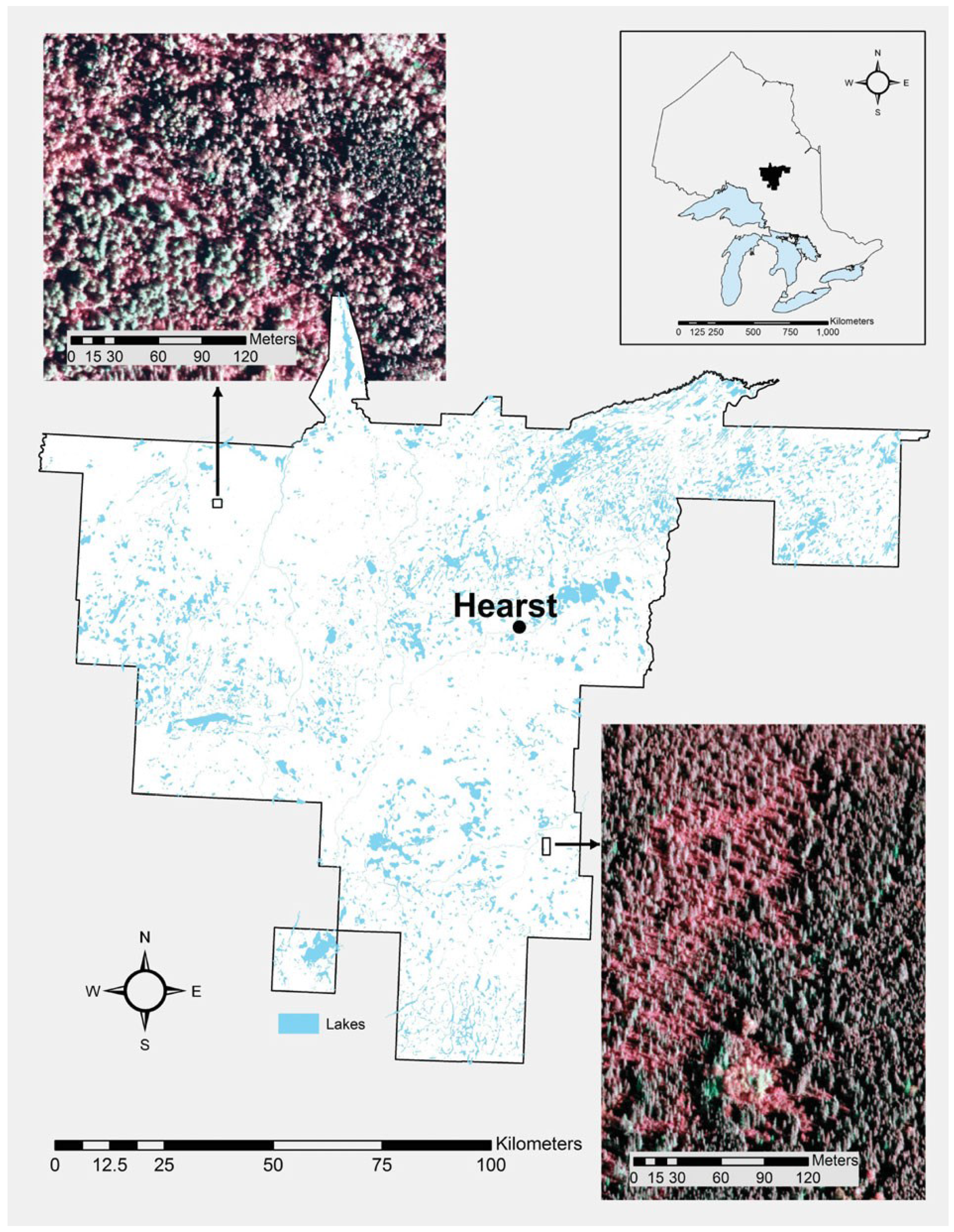
2.1. Study Area

| Forest Type | Description |
|---|---|
| SB | Nearly pure black spruce growing on wet, deep organic soils |
| LC | Mixtures of black spruce, larch and/or cedar growing on wet, deep organic soils |
| PJ | Nearly pure stands of jack pine and mixed stands of jack pine/black spruce growing on dry to moist sandy to coarse loamy soils |
| SP | Upland black spruce on fresh to moist mineral soils |
| SF | Mixed conifer stands of white spruce, balsam fir, black spruce and cedar on fresh to moist mineral soils. |
| IH | Intolerant hardwoods dominated by poplar and/or white birch |
| MWC | Mixed conifer/hardwood stands with more conifer than hardwood |
| MWH | Mixed conifer/hardwood stands with more hardwood than conifer |
2.2. Ground (Field) Data
| VCI Class | LC | MWC | MWH | PJ | IH | SB | SF | SP | Total |
|---|---|---|---|---|---|---|---|---|---|
| 0.3 | 1 (0) | 1 (0) | |||||||
| 0.4 | 1 (1) | 1 (1) | 2 (2) | ||||||
| 0.5 | 1 (0) | 1 (0) | 4 (1) | 8 (2) | 5 (1) | 3 (1) | 22 (5) | ||
| 0.6 | 8 (4) | 6 (2) | 5 (2) | 11 (3) | 17 (3) | 57 (3) | 20 (3) | 7 (2) | 131 (22) |
| 0.7 | 8 (4) | 16 (3) | 26 (4) | 11 (2) | 24 (4) | 37 (3) | 9 (2) | 17 (4) | 148 (26) |
| 0.8 | 8 (3) | 9 (2) | 8 (2) | 6 (1) | 1 (1) | 1 (0) | 33 (9) | ||
| Total | 17 (8) | 31 (8) | 40 (8) | 35 (8) | 47 (8) | 102 (8) | 36 (8) | 29 (8) | 337 (64) |
| Forest Type | N | Basal Area (m2/ha) | Total Stem Volume (m3/ha) | Top Height (m) | Quadratic Mean Dbh (cm) |
|---|---|---|---|---|---|
| LC | 25 | 38.4 (20.1–62.3) | 190 (67–380) | 15.5 (8.8–22.2) | 13.0 (6.2–23.2) |
| MWC | 39 | 29.1 (11.7–44.8) | 198 (43–338) | 19.3 (7.7–28.4) | 14.5 (5.8–31.8) |
| MWH | 48 | 29.0 (8.3–57.6) | 212 (44–520) | 19.8 (13.9–27.4) | 15.7 (7.7–26.1) |
| PJ | 43 | 28.6 (4.7–45.9) | 208 (24–401) | 17.4 (10.5–26.3) | 13.5 (6.9–23.5) |
| IH | 55 | 29.1 (10.0–55.3) | 230 (51–542) | 19.9 (13.4–28.9) | 15.5 (7.1–30.7) |
| SB | 110 | 28.9 (11.8–51.8) | 161 (53–366) | 15.5 (10.5–20.9) | 11.3 (5.3–20.2) |
| SF | 44 | 30.4 (10.8–50.0) | 162 (39–319) | 15.6 (8.6–24.6) | 11.9 (4.8–23.8) |
| SP | 37 | 31.6 (17.6–52.9) | 191 (60–363) | 17.0 (8.3–21.3) | 12.4 (6.0–19.5) |
2.3. ALS Data
| Parameter | ALS | Aerial Imagery |
|---|---|---|
| Sensor | Leica ALS50 | Leica ADS40 |
| Platform | Cessna 310 | Cessna 310 |
| Pulse rate | 119,000 Hz | |
| Scan rate | 32 Hz | |
| Field of view | 30° | 42° |
| Flying height | 2,400 m | 2,400 m |
| Line spacing | 1,000 m | 3,000 m |
| Overlap | 20% | 30% (max) |
| Vertical accuracy | < 30 cm | |
| Pulse density | ~1.0/m2 | 2.4/m2 |
| Field name | Description | ALS | IPC |
|---|---|---|---|
| MEAN | Mean height (m) | √ | √ |
| STD_DEV_95 | Standard deviation | √ | √ |
| ABS_DEV_95 | Absolute standard deviation | √ | √ |
| SKEW_95 | Skewness | √ | √ |
| KURTOSIS_95 | Kurtosis | √ | √ |
| P10 | First Decile ALS height (m) | √ | √ |
| P20 | Second Decile ALS height (m) | √ | √ |
| ↓ | ↓ | ↓ | |
| P80 | Eighth decile ALS height (m) | √ | √ |
| P90 | Ninth decile ALS height (m) | √ | √ |
| MAX | Maximum height (m) | ||
| D1 | Cumulative percentage of the number of returns found in bin 1 of 10 | √ | √ |
| D2 | Cumulative percentage of the number of returns found in bin 2 of 10 | √ | √ |
| ↓ | ↓ | ↓ | |
| D8 | Cumulative percentage of the number of returns found in bin 8 of 10 | √ | √ |
| D9 | Cumulative percentage of the number of returns found in bin 9 of 10 | √ | √ |
| DA_95 | First returns/ all returns | √ | |
| DV_95 | First vegetation returns/all returns | √ | √ |
| DB_95 | First and only return / all returns | √ | |
| VDR_95 | Vertical distribution ratio = [max−median]/max | √ | √ |
| Covar_95 | Std Dev (all returns)/ mean (all returns) | √ | |
| CanCovar_95 | Std Dev (first returns only)/ mean (first returns only) | √ | √ |
| VCI_95 | Vertical complexity index [ 20] | √ | √ |
| cc2 | Crown closure: the number of 2 m × 2 m canopy height model raster cells that have a height value greater or equal to 2 m divided by the number of nonvoid 2 m × 2 m cells, expressed as a percen t | √ | √ |
| ↓ | ↓ | ↓ | |
| cc26 | Crown closure: the number of 2 m × 2 m canopy height model raster cells that have a height value greater or equal to 26 m divided by the number of nonvoid 2 m × 2 m cells, expressed as a percen | √ | √ |
| cc28 | Crown closure: the number of 2 m × 2 m canopy height model raster cells that have a height value greater or equal to 28 m divided by the number of nonvoid 2 m × 2 m cells, expressed as a percen | √ | √ |
| TD2 | Cumulative percentage of vegetation returns 0-2m | √ | |
| TD4 | Cumulative percentage of vegetation returns 0-4m | √ | |
| ↓ | ↓ | ||
| TD30 | Cumulative percentage of vegetation returns 0-30m | √ | |
| s2 | % of vegetation returns in slice 0-2m | √ | |
| s4 | % of vegetation returns in slice 2-4m | √ | |
| ↓ | ↓ | ||
| s30 | % of vegetation returns in slice 28-30m | √ |
2.4. Image-Based Data
3. Methods
3.1. Dependent Variables
3.2. Independent ALS and Optical CHM Predictors

3.3. Parametric or Non-Linear Regression (NLS)
3.4. Non Parametric or RandomForest Nearest Neighbour Prediction
3.5. Evaluating Fit
- H0: ALS = IPC. The error index does not depend on remote sensing technique (ALS vs. IPC).
- H1: ALS ≠ IPC. The error index depends on remote sensing technique (ALS vs. IPC).
- and
- H0: SUR = RFNN. The error index does not depend on statistical technique (SUR vs. RFNN).
- H1: SUR ≠ RFNN. The error index depends on statistical technique (SUR vs. RFNN).
4. Results
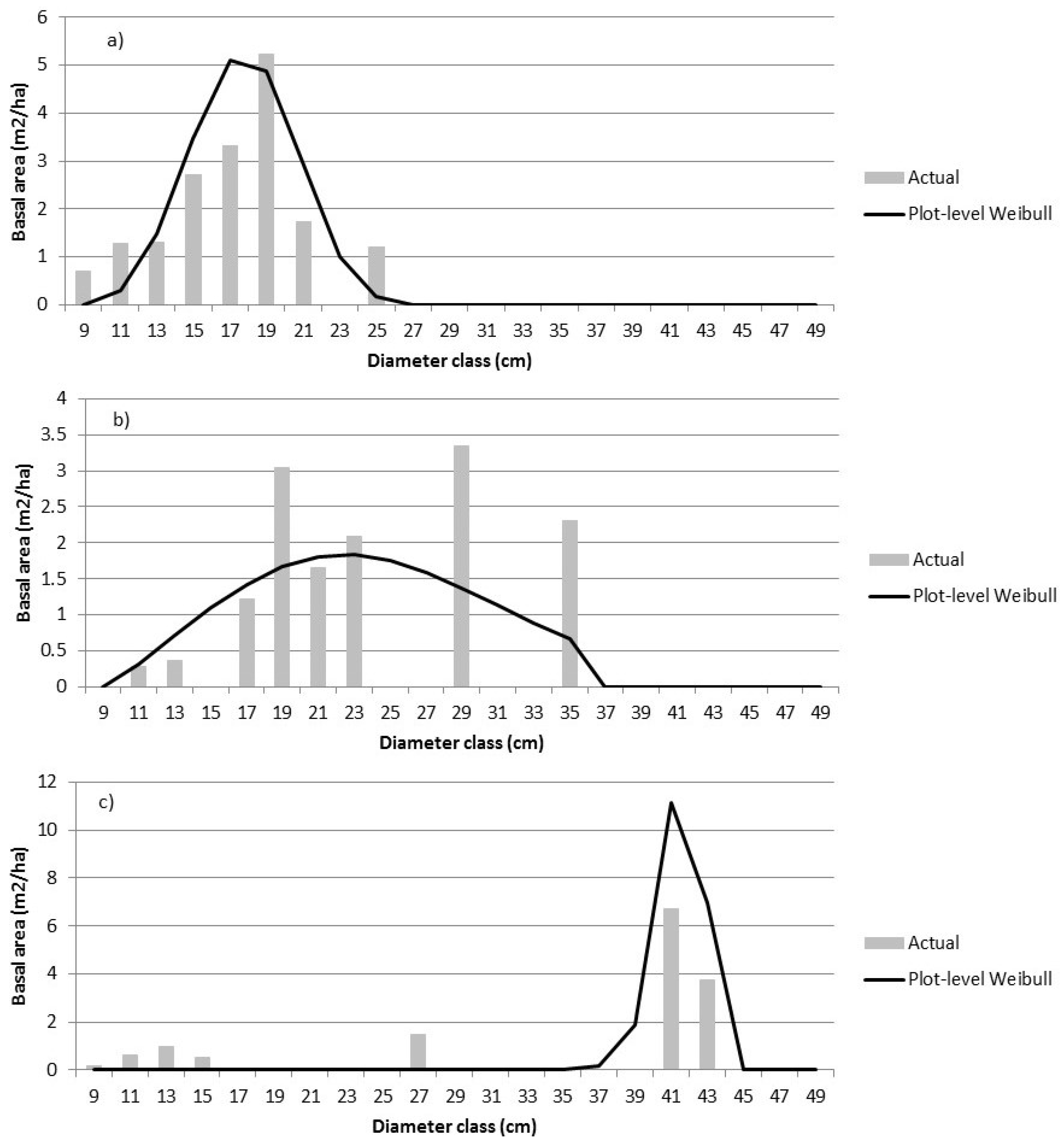
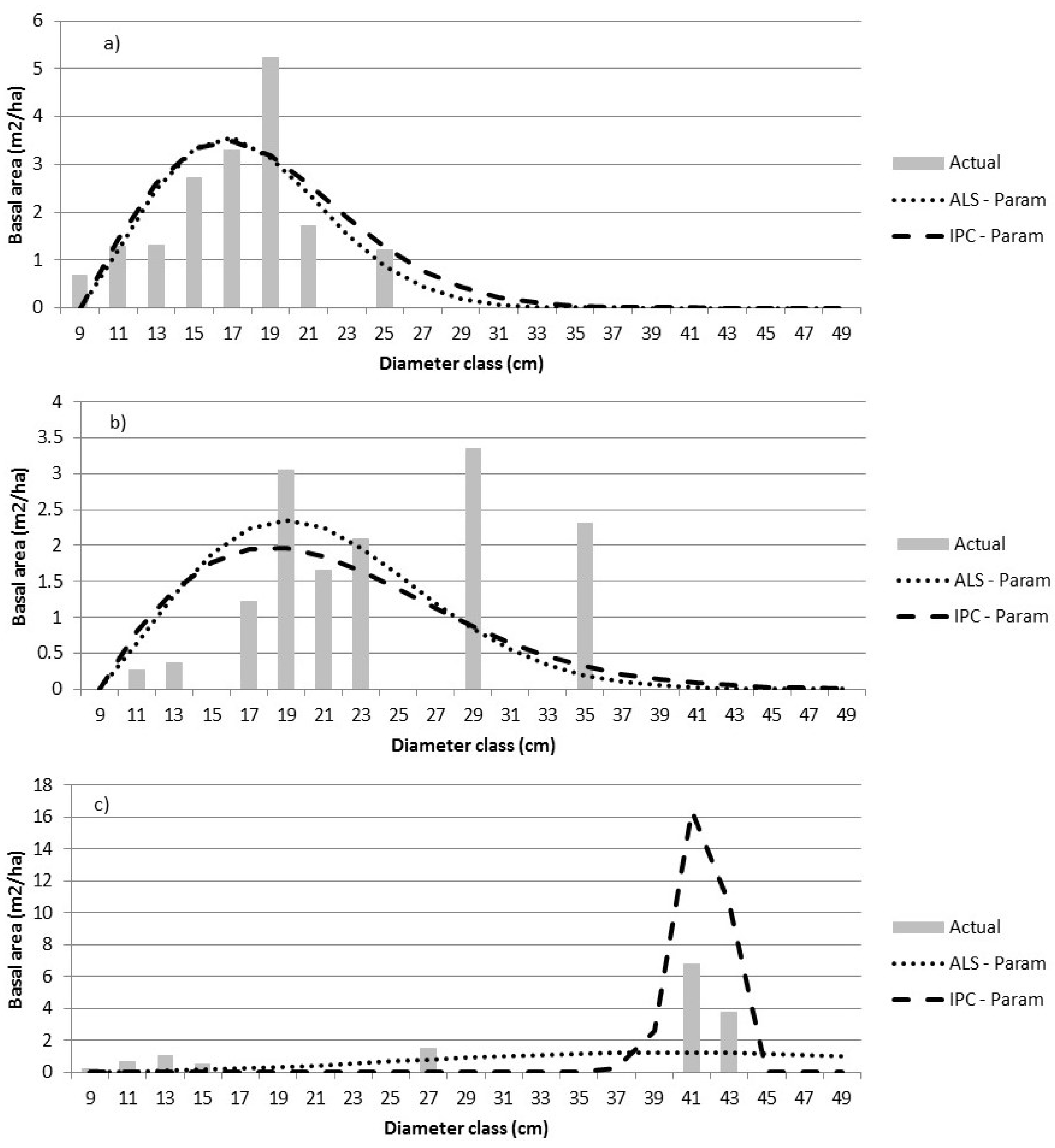
4.1. Parametric Predictions

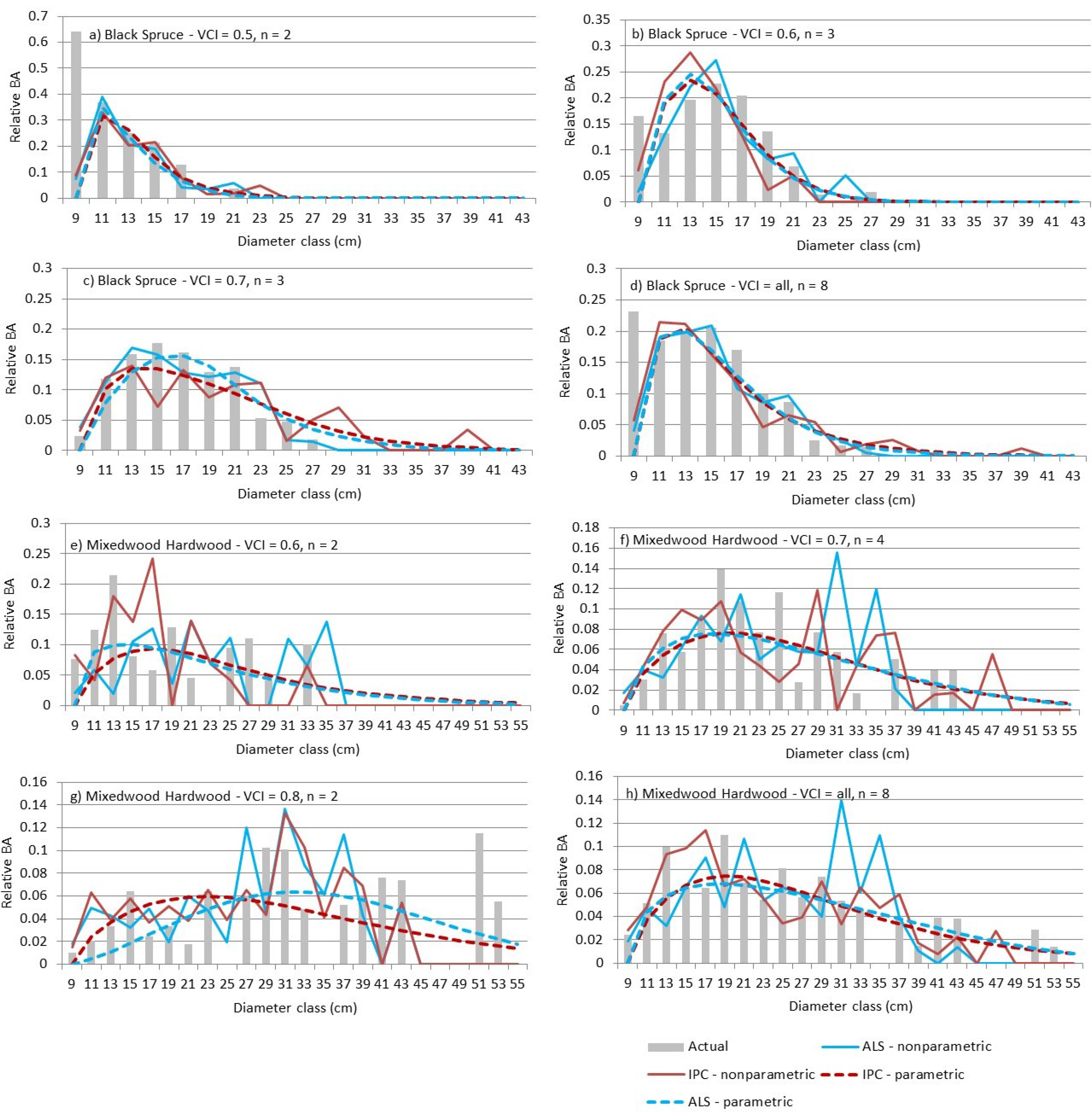
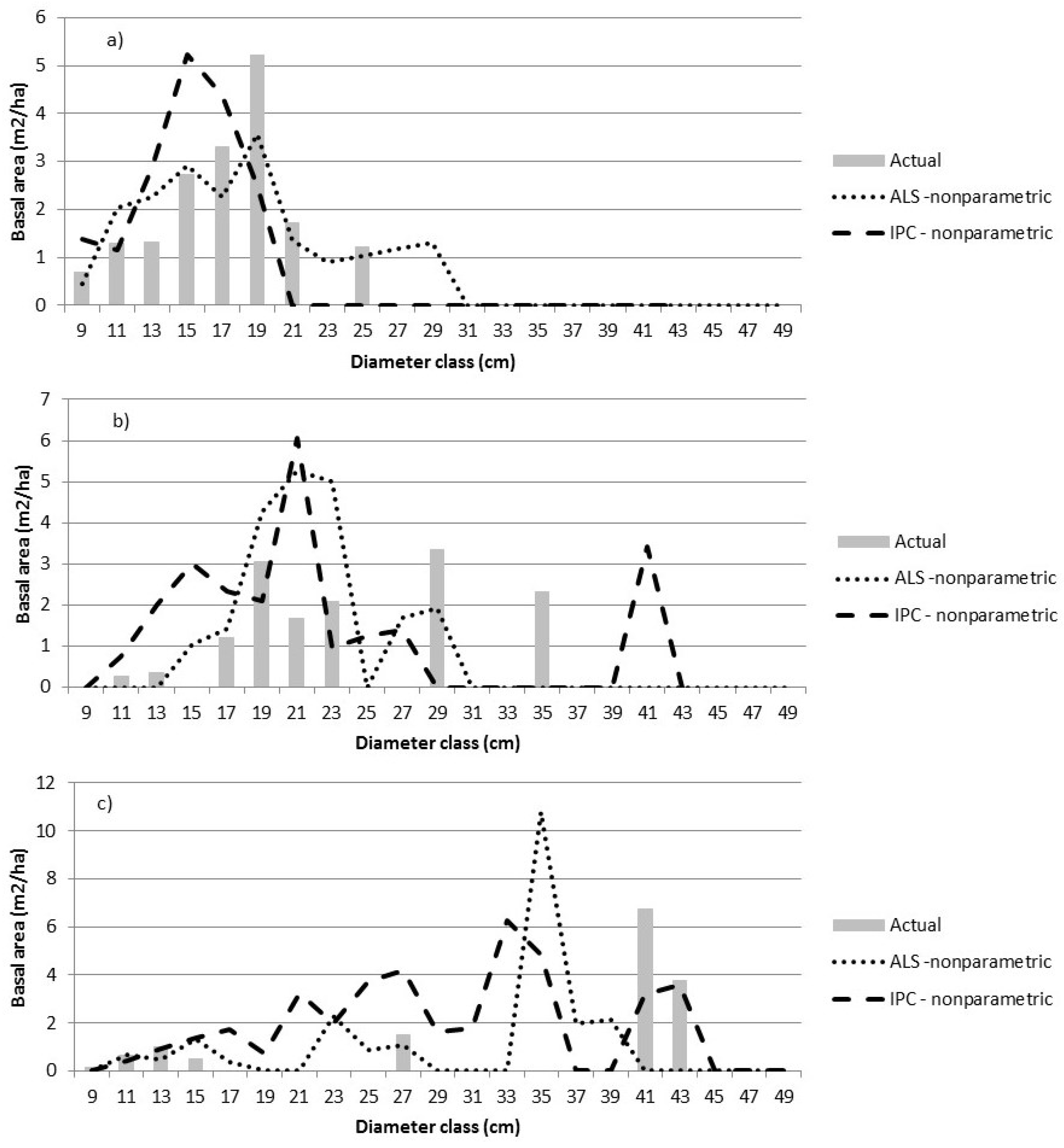
4.2. Nonparametric Predictions

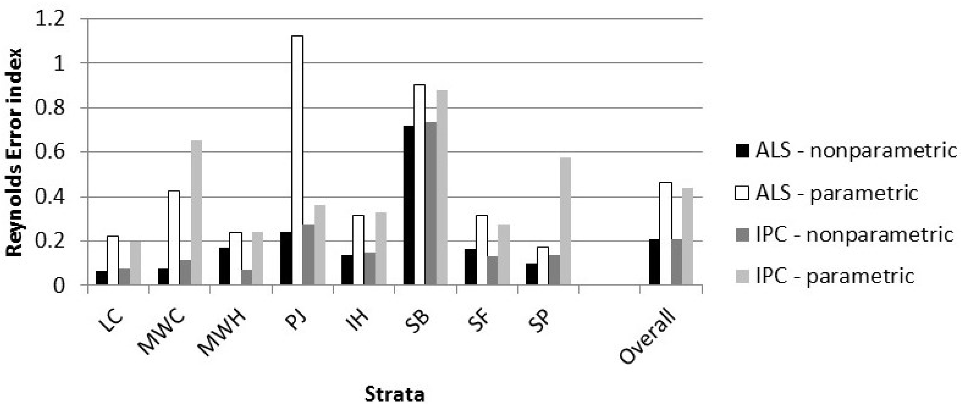
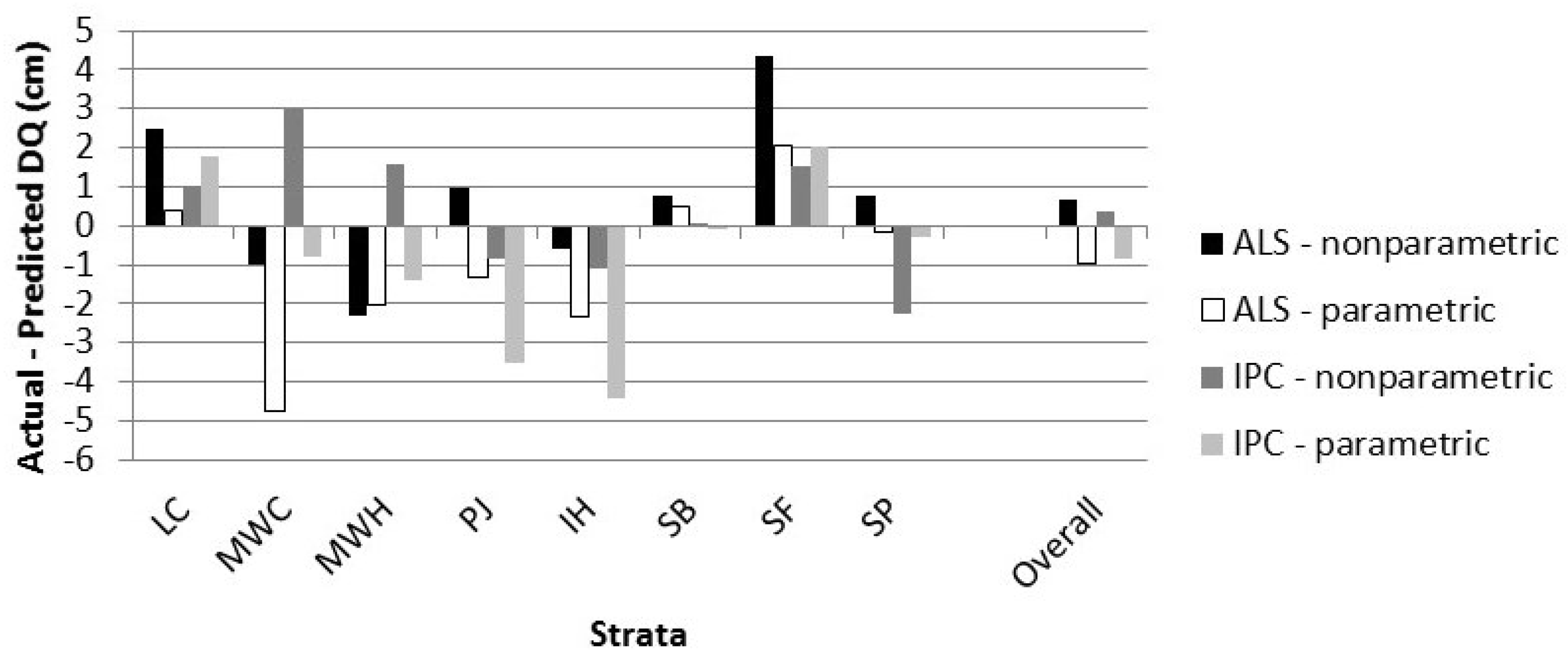
4.3. Measures of Fit

| Error Index | Error Index | DQ Error | |
|---|---|---|---|
| Remote sensing technique (RS) | H0: ALS = IPC | 0.6048 | 0.8096 |
| H0: no forest type effect | 0.0449 | 0.4541 | |
| Statistical technique (S) | H0: SUR = RFNN | <0.0001 | 0.0145 |
| H0: no forest type effect | 0.3161 | 0.3770 | |
| RS x S interaction | H0: no interaction | 0.6128 | 0.8660 |
| H0: no forest type effect | 0.0199 | 0.1812 |
5. Discussion
6. Conclusions
Acknowledgments
Conflict of Interest
References
- Næsset, E. Estimating timber volume of forest stands using airborne laser scanner data. Remote Sens. Environ. 1997, 61, 246–253. [Google Scholar] [CrossRef]
- Woods, M.; Pitt, D.; Lim, K.; Nesbitt, D.; Etheridge, D.; Penner, M.; Treitz, P. Operational implementation of a LiDAR inventory in Boreal Ontario. For. Chron. 2011, 87, 512–528. [Google Scholar] [CrossRef]
- Pitt, D.G.; Woods, M.; Penner, M. A comparison of point clouds derived from stereo imagery and airborne laser scanning for the area-based estimation of forest inventory attributes in boreal Ontario. Can. J. Rem. Sen. 2014, 40, 214–232. [Google Scholar] [CrossRef]
- Bailey, R.L.; Dell, T.R. Quantifying diameter distributions with the Weibull function. For. Sci. 1973, 19, 97–103. [Google Scholar]
- Thomas, V.; Oliver, R.D.; Lim, K.; Woods, M. LiDAR and Weibull modeling of diameter and basal area. For. Chron. 2008, 84, 866–875. [Google Scholar] [CrossRef]
- Cao, Q.V. Predicting parameters of a Weibull function for modeling diameter distribution. For. Sci. 2004, 50, 682–685. [Google Scholar]
- Kangas, A.; Maltamo, M. Calibrating predicted diameter distribution with additional information. For. Sci. 2010, 46, 390–396. [Google Scholar]
- Breidenbach, J.; Gläser, C.; Schmidt, M. Estimation of bivariate diameter and height distributions using ALS. In SilviLaser 2008: 8th International Conference on LiDAR: Applications in forest assessment and inventory, Heriot-Watt University, Edinburgh, UK, 17–19 September 2008; pp. 366–372.
- Magnussen, S.; Næsset, E.; Gobakken, T. Prediction of tree size distributions and inventory variables from cumulants of canopy height distributions. Forestry 2013, 86, 583–595. [Google Scholar] [CrossRef]
- McRoberts, R. Estimating forest attribute parameters for small areas using nearest neighbours techniques. Fore. Ecol. Mgmt. 2012, 272, 3–12. [Google Scholar] [CrossRef]
- Eskelson, B.N.I.; Temesgen, H.; LeMay, V.; Barrett, T.; Crookston, N.; Hudak, A. The roles of nearest neighbour methods in imputing missing data in forest inventory and monitoring databases. Scand. J. For. Res. 2009, 24, 235–234. [Google Scholar] [CrossRef]
- Temesgen, H.; LeMay, V.; Froese, K.; Marshall, P. Imputing tree-lists from aerial attributes for complex stands of south-eastern British Columbia. For. Ecol. Mgmt. 2003, 177, 277–285. [Google Scholar] [CrossRef]
- Guindon, L.; Ung, C.-H.; Beaudoin, A.; Miranda, M.; Villemaire, P.; Patry, A. Predicting stand table in a mixed forest of southern Quebec with airborne LiDAR using the kNN method. In Proceedings of the IUFRO Conference on Extending Forest Inventory and Monitoring over Space and Time, Quebec City, Canada, 19–22 May 2009; p. 5.
- Hudak, A.; Crookston, N.; Evans, J.; Hall, D.; Fallowski, M. Nearest neighbour imputation of species-level, plot-scale forest structure attributes from LiDAR data. Remo. Sens. Environ. 2008, 112, 2232–2245. [Google Scholar] [CrossRef]
- Magnussen, S.; Eggermont, P.; LaRiccia, V.N. Recovering Tree Heights from Airborne Laser Scanner Data. For. Sci. 1999, 45, 407–422. [Google Scholar]
- Mehtätalo, L.; Nyblom, J. Estimating Forest Attributes Using Observations of Canopy Height: A Model-Based Approach. For. Sci. 2009, 55, 411–422. [Google Scholar]
- Mehtätalo, L.; Nyblom, J. A Model-Based Approach for Airborne Laser Scanning Inventory: Application for Square Grid Spatial Pattern. For. Sci. 2012, 58, 106–118. [Google Scholar] [CrossRef]
- Bollandsås, O.; Maltamo, M.; Gobakken, T.; Naesset, E. Comparing parametric and non-parametric modelling of diameter distributions on independent data using airborne laser scanning in a boreal conifer forest. Forestry 2013, 86, 493–501. [Google Scholar] [CrossRef]
- Packalén, P.; Maltamo, M. Estimation of species-specific diameter distributions using airborne laser scanning and aerial photographs. Can. J. For. Res. 2008, 38, 1750–1760. [Google Scholar] [CrossRef]
- Hearst Forest Management Inc. Forest Management Plan for the Hearst Forest. Available online: http://www.hearstforest.com/english/PDF/HearstForest2007FMP.pdf (accessed on 3 November 2015).
- Van Ewijk, K.Y.; Treitz, P.M.; Scott, N.A. Characterizing forest succession in central Ontario using Lidar-derived indices. Photogramm. Eng. Rem. Sens. 2011, 77, 261–269. [Google Scholar] [CrossRef]
- Shannon, C.E. The mathematical theory of communication. Bell Syst. Tech. J. 1948, 27, 379–423. [Google Scholar] [CrossRef]
- Bollandsås, O.; Naesset, E. Estimating percentile-based diameter distributions in uneven-sized Norway spruce stands using airborne laser scanner data. Scan. J. For. Res. 2007, 22, 33–47. [Google Scholar] [CrossRef]
- Valbuena, R.; Packalen, P.; Mehtätalo, L.; Garcia-Abril, A.; Maltamo, M. Characterizing forest structural types and shelterwood dynamics from Lorenz-based indicators predicted by airborne laser scanning. Can. J. For. Res. 2013, 43, 1063–1074. [Google Scholar] [CrossRef]
- Ontario Ministry of Natural Resources. Ontario Forest Resources Inventory Calibration Plot Specifications—Revised; Ontario Ministry of Natural Resources Internal Publication: Ontario, Canada, 2012; p. 41. [Google Scholar]
- Ontario Ministry of Natural Resources. Ontario Forest Resources Inventory Photo Interpretation Specifications—Revised; Ontario Ministry of Natural Resources Internal Publication: Ontario Canada, 2012; p. 87. [Google Scholar]
- Hirschmüller, H. Stereo processing by semiglobal matching and mutual information. IEEE T. Pattern Anal. Mach. Intell. 2008, 30, 328–341. [Google Scholar] [CrossRef] [PubMed]
- Gehrke, S.; Morin, K.; Downey, M.; Boehrer, N.; Fuchs, T. Semi-Global matching: An alternative to LiDAR for DSM generation? Int. Arch. Photogramm. Remote Sens. 2010, 38. Part B1. [Google Scholar]
- Gehrke, S.; Uebbing, R.; Downey, M.; Morin, K. Creating and using very high density point clouds derived from ADS imagery. In Proceedings of the American Society of Photogrammetry and Remote Sensing 2011 Annual Conference, Milwaukee, WI, USA, 1–5 May 2011.
- Gehrke, S.; Downey, M.; Uebbing, R.; Welter, J.; LaRocque, W. A multi-sensor approach to semi-global matching. In International Archives of the Photogrammetry, Remote Sensing and Spatial Information Sciences, 2012 XXII ISPRS Congress, Melbourne, Australia, 25 August–1 September 2012; XXXIX-B3, pp. 17–22.
- Penner, M.; Pitt, D.G.; Woods, M.E. Parametric vs nonparametric LiDAR models for operational forest inventory in boreal Ontario. Can. J. Rem. Sens. 2013, 39, 426–443. [Google Scholar]
- Kraus, K.; Pfeifer, N. Determination of terrain models in wooded areas with airborne laser scanner data. ISPRS J. Photogramm. Remote Sens. 1998, 53, 193–203. [Google Scholar] [CrossRef]
- Liaw, A.; Wiener, M. Classification and Regression by randomForest. R News 2002, 2, 18–22. [Google Scholar]
- Crookston, N.I.; Finley, A.O. Yaimpute: An R package for kNN imputation. J. Stat. Softw. 2008, 23, 1–16. [Google Scholar] [CrossRef]
- Reynolds, M.R., Jr.; Burk, T.E.; Huang, W.-C. Goodness-of-fit tests and model selection procedures for diameter distribution models. For. Sci. 1988, 34, 373–399. [Google Scholar]
- Reichmann, R.; Wilson, B.; Lister, A.; Parks, S. An effective assessment protocol for continuous geospatial datasets of forest characteristics using USFS Forest Inventory and Analysis (FIA) data. Rem. Sens. Environ. 2010, 114, 2337–2353. [Google Scholar] [CrossRef]
- MultiDatTM. Available online: http://www.castonguay.biz (accessed on 15 July 2015).
- Leckie, D.; Gougeon, F.; Hill, D.; Quinn, R.; Armstrong, L.; Shreenan, R. Combined high-density lidar and multispectral imagery for individual tree crown analysis. Can. J. Rem. Sens. 2003, 20, 633–649. [Google Scholar] [CrossRef]
- Salas, C.; Ene, L.; Gregoire, T.G.; Næsset, E.; Gobakken, T. Modelling tree diameter from airborne laser scanning derived variable: A comparison of spatial statistical models. Remote Sens. Environ. 2010, 114, 1277–1285. [Google Scholar] [CrossRef]
- Peuhkurinen, J.; Mehtätalo, L.; Maltamo, M. Comparing individual tree detection and the area-based statistical approach for the retrieval of forest stand characteristics using airborne laser scanning in scots pine stands. Can. J. For. Res. 2011, 41, 583–598. [Google Scholar] [CrossRef]
- Xu, Q.; Hou, Z.; Maltamo, M.; Tokola, T. Calibration of area based diameter distribution with individual tree based diameter estimates using airborne laser scanning. IPRS J. Photogramm. Remote Sens. 2014, 93, 65–76. [Google Scholar] [CrossRef]
© 2015 by the authors; licensee MDPI, Basel, Switzerland. This article is an open access article distributed under the terms and conditions of the Creative Commons Attribution license (http://creativecommons.org/licenses/by/4.0/).
Share and Cite
Penner, M.; Woods, M.; Pitt, D.G. A Comparison of Airborne Laser Scanning and Image Point Cloud Derived Tree Size Class Distribution Models in Boreal Ontario. Forests 2015, 6, 4034-4054. https://doi.org/10.3390/f6114034
Penner M, Woods M, Pitt DG. A Comparison of Airborne Laser Scanning and Image Point Cloud Derived Tree Size Class Distribution Models in Boreal Ontario. Forests. 2015; 6(11):4034-4054. https://doi.org/10.3390/f6114034
Chicago/Turabian StylePenner, Margaret, Murray Woods, and Douglas G. Pitt. 2015. "A Comparison of Airborne Laser Scanning and Image Point Cloud Derived Tree Size Class Distribution Models in Boreal Ontario" Forests 6, no. 11: 4034-4054. https://doi.org/10.3390/f6114034
APA StylePenner, M., Woods, M., & Pitt, D. G. (2015). A Comparison of Airborne Laser Scanning and Image Point Cloud Derived Tree Size Class Distribution Models in Boreal Ontario. Forests, 6(11), 4034-4054. https://doi.org/10.3390/f6114034