Local-Scale Mapping of Biomass in Tropical Lowland Pine Savannas Using ALOS PALSAR

Abstract
:
1. Introduction
1.1. Why Map Tropical Savannas at More Local Scales?
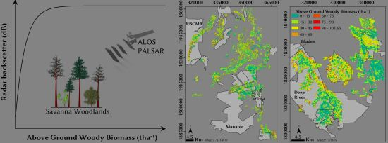
- Mapping the AGWB of over 50% of the lowland savanna woodlands of Belize at 100-m resolution, using a locally modelled relationship between the satellite radar backscatter and observations of biomass from an extensive national inventory of forest plots.
- Analysing the resulting AGWB map to quantify for the first time the variation in AGWB across the different woodland savannas within the country and exploring how this might provide forest managers with enhanced information about the nature and locality of different woodland components, compared to previous qualitative thematic mapping using the UNESCO land cover classification system.
- Examining, within a pilot study area of approximately 933 km2, whether the biomass map produced at 100 m might enable differences in biomass to be observed between forest areas that are being protected or sustainably managed, compared to unprotected forest areas.
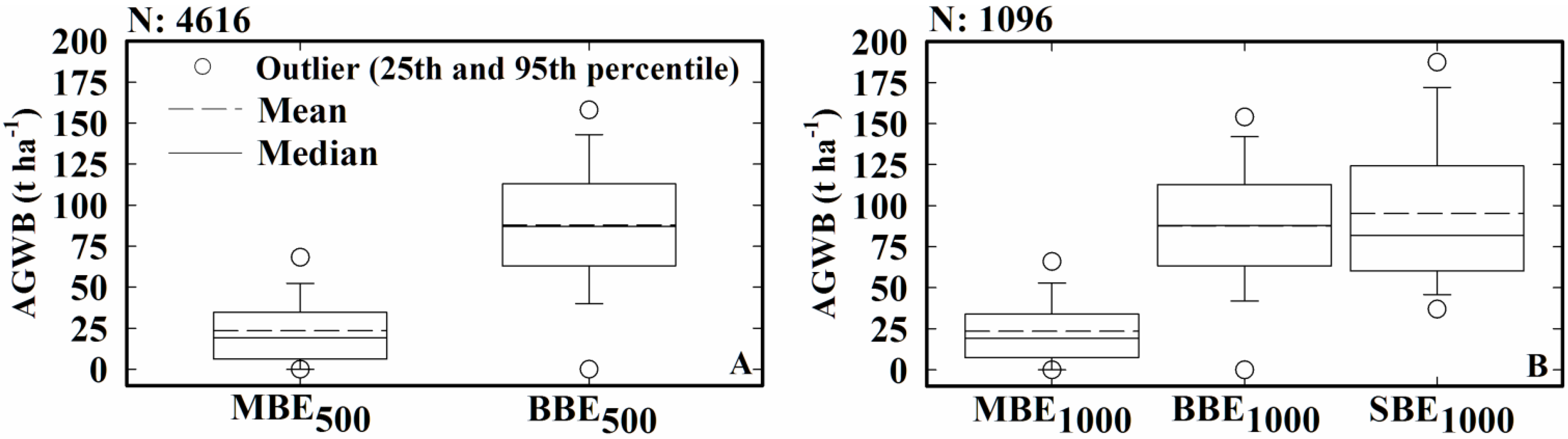
- For two specific protected areas of Belize, assessing if this finer scale mapping produces biomass estimates that accord more closely with ground measurements of biomass than estimates based on biomass values extracted from pantropical biomass data sets at 500-m and 1000-m resolution produced by [17,18].
1.2. Mapping of Savanna Woodlands with Active Satellite Earth Observation
1.3. The Use of More Detailed Mapping of Woody Biomass in Savannas
2. Experimental Section
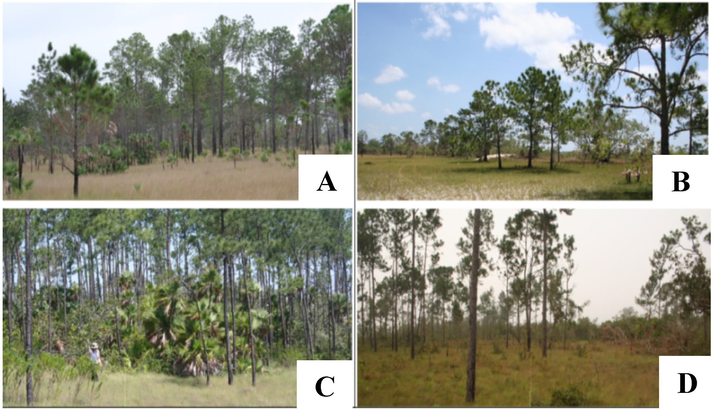
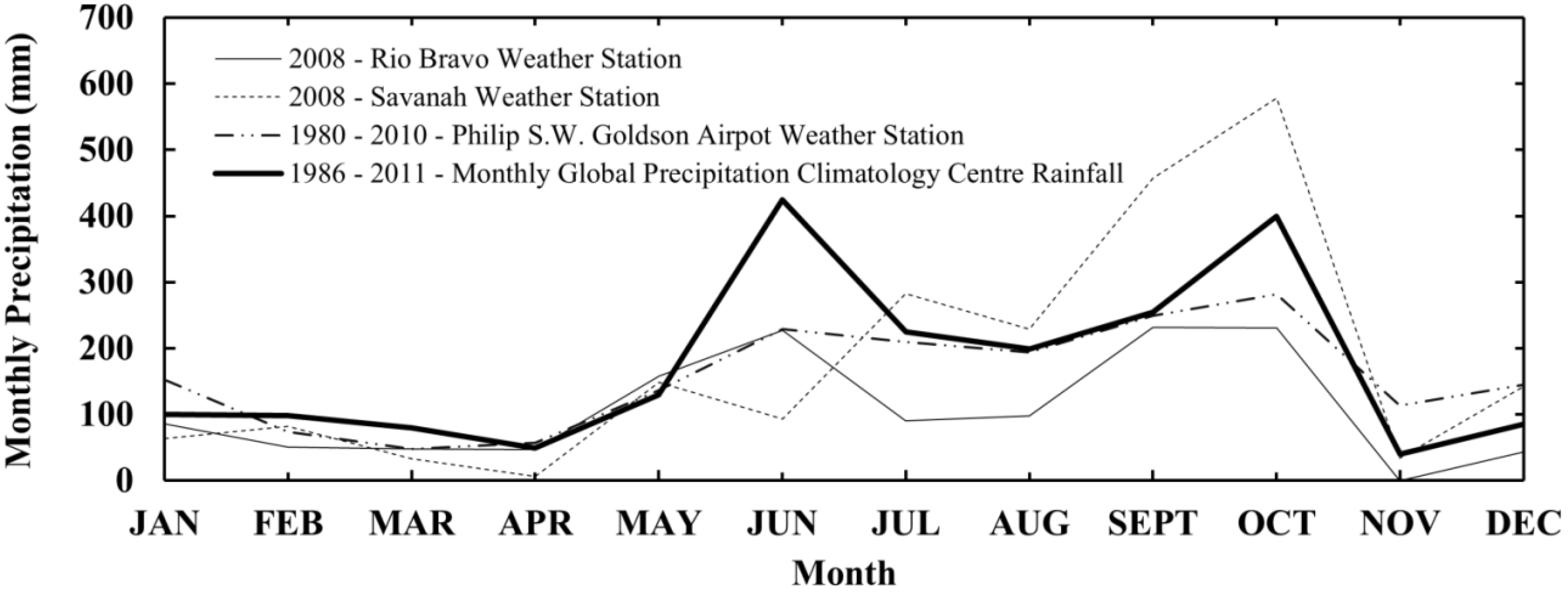
2.1. Description of the Lowland Savanna Ecosystem
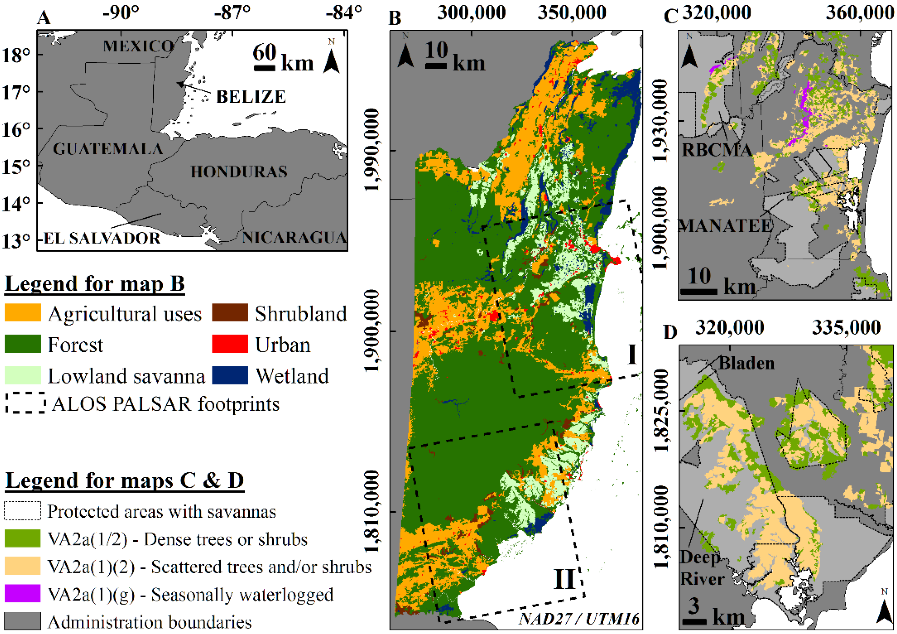


2.2. ALOS PALSAR Data
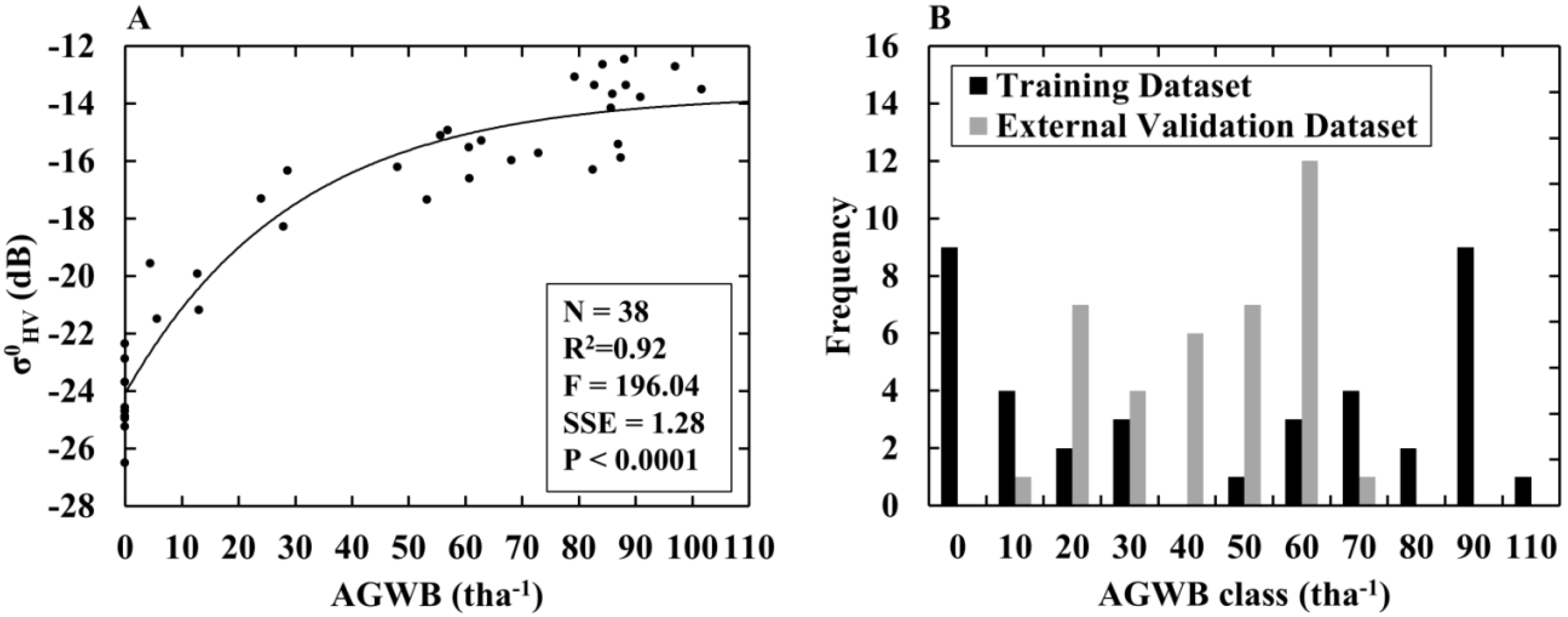
2.3. Biomass Mapping Using ALOS PALSAR and Semi-Empirical Modelling

| AGWB (tha−1) | Density (Trees ha−1) | BA (m2 ha−1) | ||||||||
|---|---|---|---|---|---|---|---|---|---|---|
| Datasets | Plot size (ha) | Range | Mean | St. Dev. | Range | Mean | SD | Range | Mean | St. Dev. |
| Training | 32 × 1 | 0–101.6 | 47.3 | 37.1 | 0–680 | 155 | 171.7 | 0–15.3 | 6.15 | 5.0 |
| 6 × 0.1 | ||||||||||
| Validation | 38 × 0.1 | 1–72 | 39.5 | 19.4 | 20–350 | 145 | 75.1 | 0–11.0 | 5.7 | 2.6 |
2.4. Deriving Ground-Based Estimates of AGWB for Two Protected Areas
| AGWB (t ha−1) | Density (Trees ha−1) | BA (m2 ha−1) | ||||||||
|---|---|---|---|---|---|---|---|---|---|---|
| Data | Plot size (ha) | Range | Mean | SD | Range | Mean | SD | Range | Mean | SD |
| DR | 62 × 0.1 | 2.25–76.19 | 31.60 | 17.78 | 20–350 | 121 | 70.40 | 0.5–11.25 | 6.15 | 2.54 |
2.5. Classification of Savannas by Protection and Management Type
2.6. Comparing the New Mapping with National Level Carbon Stock Maps from Pantropical Data Sets
| Biomass map | EO data used | Algorithm | Pixel size (m) | Reduced resolution (m) | Compared to |
|---|---|---|---|---|---|
| MBE100 | ALOS PALSAR | Semi-empirical water cloud model | 100 | 500 | BBE500 BBE1000 SBE1000 |
| 1000 | |||||
| BBE500 | ICESAT GLAS MODIS Bidirectional Reflectance Distribution Function BDRF SRTM | RandomForests | 500 | 1000 | MBE500 |
| SBE1000 | |||||
| SBE1000 | ICESAT GLAS MODIS LAI/NDVI/Vegetation Continuous Fields VCT SRTM QUICKSAT | MaxEnt | 1000 | - | MBE1000 |
| BBE1000 |
3. Results and Discussion
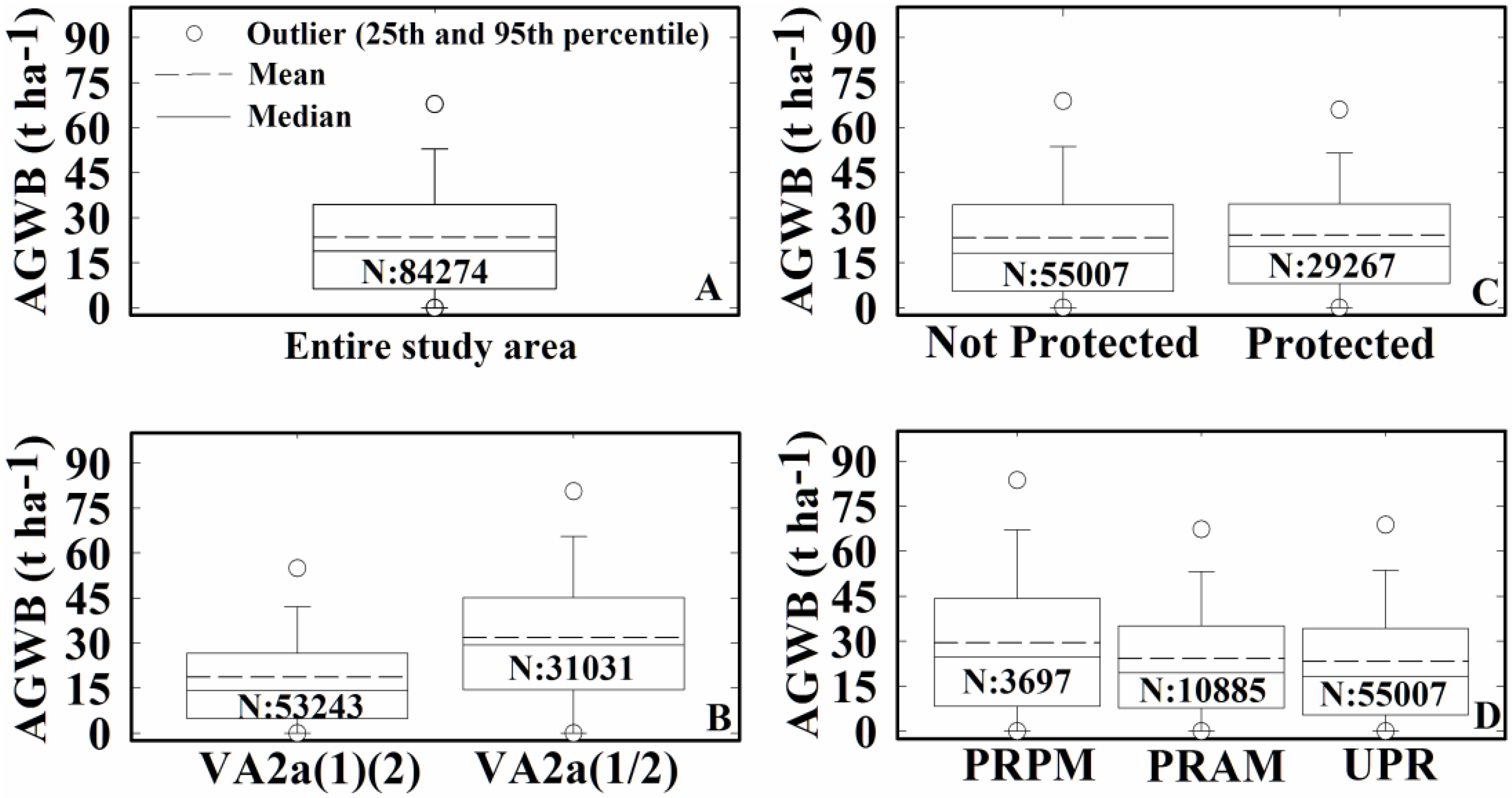
3.1. Evaluating the AGWB of the Lowland Savannas per Protection and Management

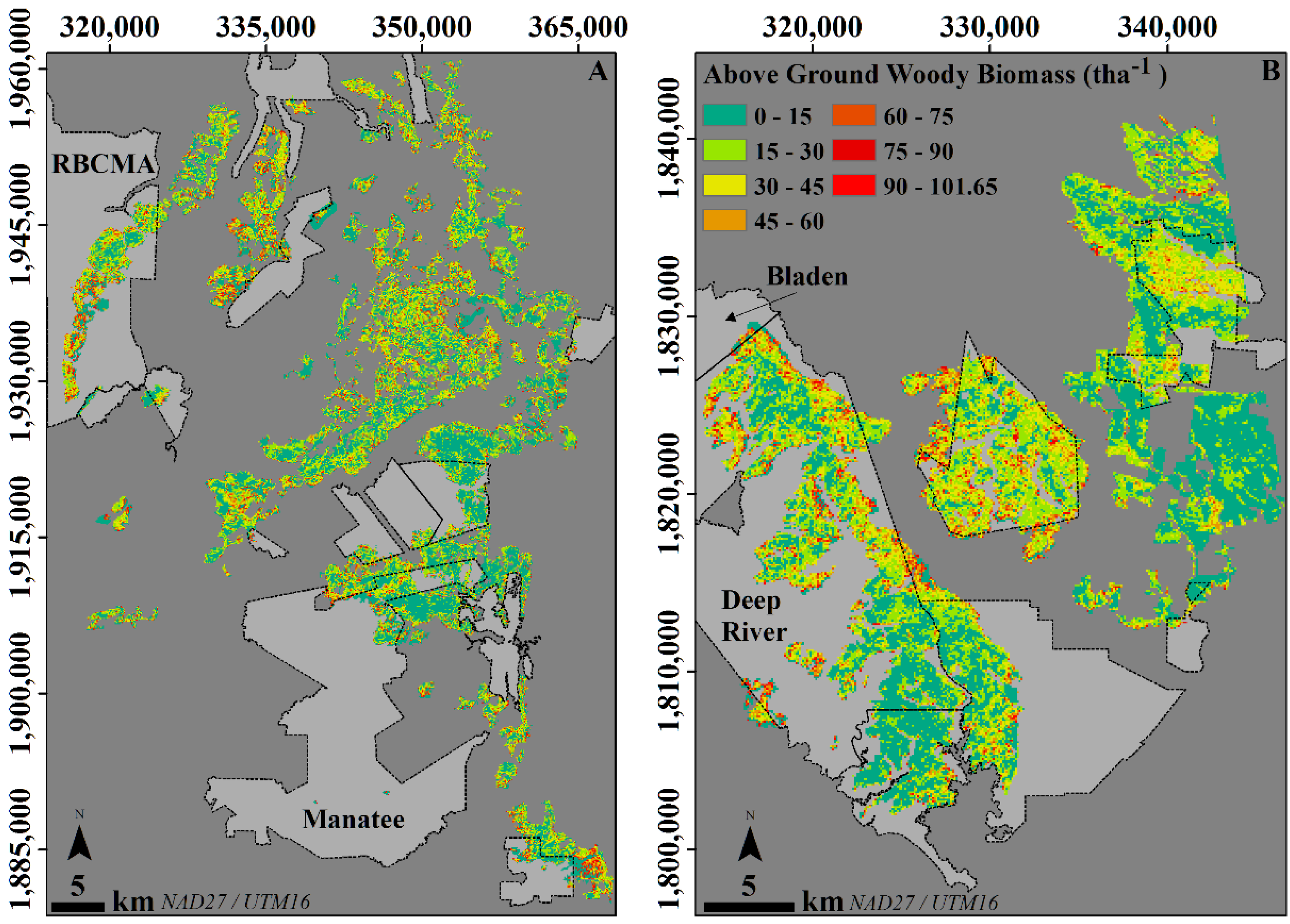
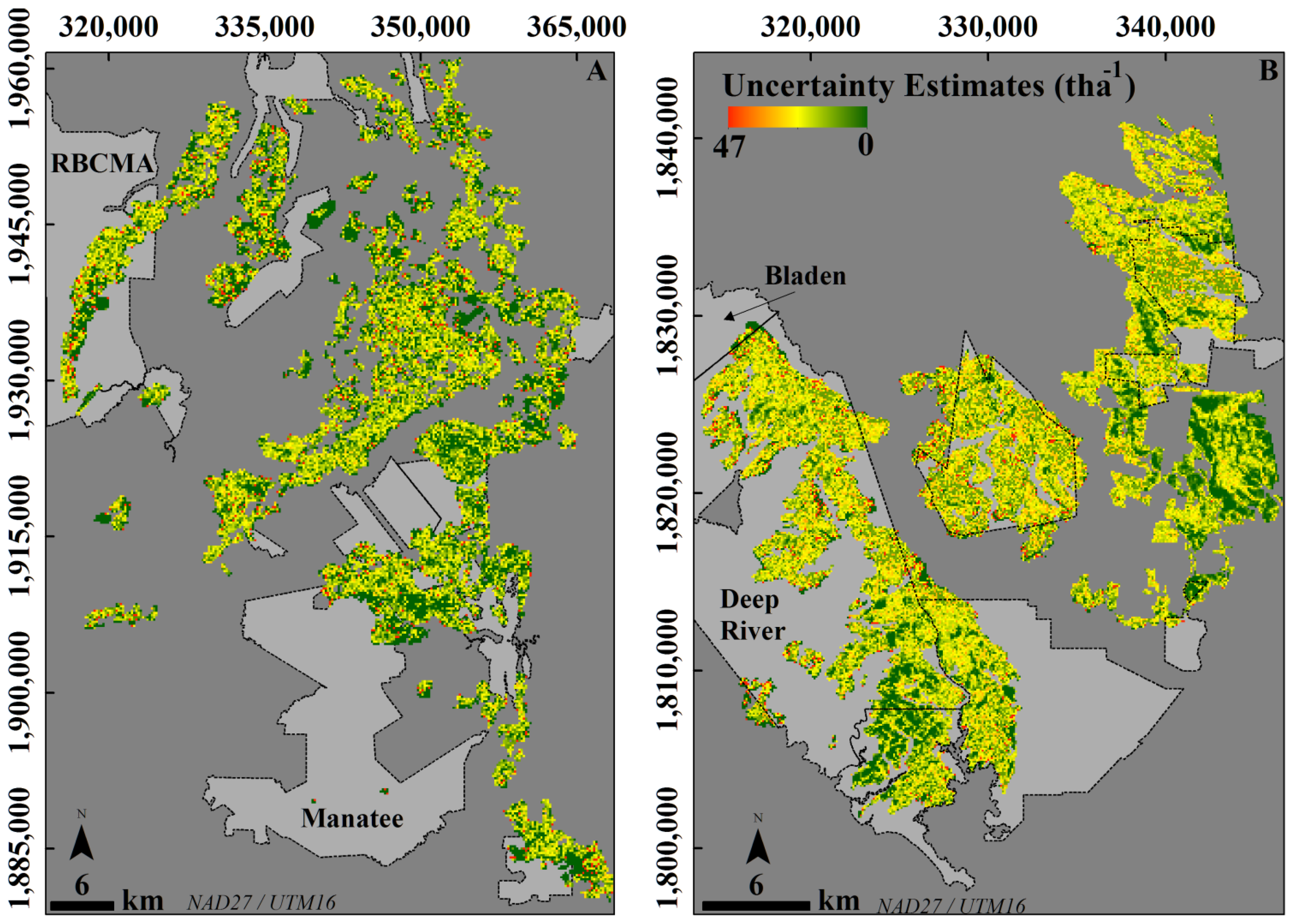
3.2. Using the Map to Characterize AGWB in the Lowland Savannas of Belize

| Estimated Uncertainty (tha−1) | ||||||||
|---|---|---|---|---|---|---|---|---|
| 0–15 | 4 (V) | 10.84 | 14.2 | 131 | 35,425 | 6.75 | 19.64 | 14.21 |
| 15–30 | 8 (V) | 20.60 | 16.02 | 78 | 22,758 | 17.21 | 23.40 | 20.67 |
| 30–45 | 11 (V) | 38.88 | 7.43 | 19 | 13,774 | 6.96 | 8.55 | 7.79 |
| 45–60 | 9 (V) | 51.98 | 15.13 | 29 | 6247 | 14.93 | 17.40 | 16.48 |
| 60–75 | 6 (V) | 66.30 | 14.62 | 22 | 3014 | 14.66 | 16.50 | 15.64 |
| 75–90 | 10 (T) | 85.10 | 43.8 | 51.47 | 1489 | 42.00 | 45.90 | 43.86 |
| 90–105 | 3 (T) | 96.51 | 25.58 | 26.51 | 1567 | 26.81 | 27.45 | 27.45 |
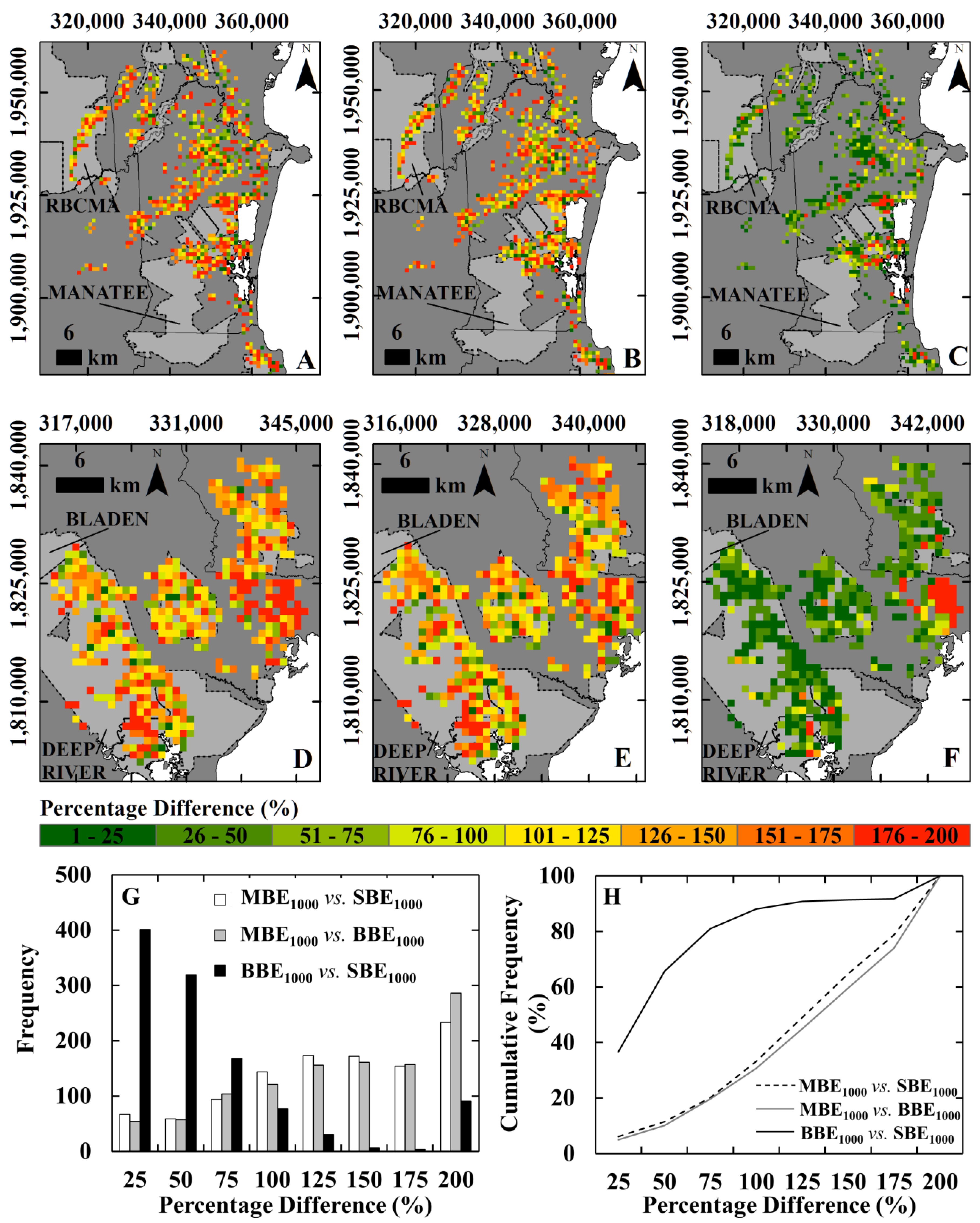
3.3. Comparison of the Local Map Estimates with Pantropical Carbon Stock Maps
4. Conclusions
Acknowledgments
Author Contributions
Conflicts of Interest
References and Notes
- Grace, J.; José, J.S.; Meir, P.; Miranda, H.S.; Montes, R.A. Productivity and carbon fluxes of tropical savannas. J. Biogeogr. 2006, 33, 387–400. [Google Scholar]
- Ratnam, J.; Bond, W.J.; Fensham, R.J.; Hoffman, W.A.; Archibald, S.; Lehmann, C.E.R.; Anderson, M.T.; Higgins, S.I.; Sankaran, M. When is a ‘forest’ a savannas, and why does it matter? Glob. Ecol. Biogeogr. 2011, 20, 653–660. [Google Scholar] [CrossRef]
- FAO. Global Forest Resources Assessment, Main Report; Food and Agriculture Organization of the United Nations: Rome, Italy, 2010. [Google Scholar]
- Furley, P. Tropical savannas: Biomass, plant ecology, and the role of fire and soil on vegetation. Progr. Phys. Geogr. 2010, 34, 563–585. [Google Scholar] [CrossRef]
- Castro, E.A.; Kauffman, J.B. Ecosystem structure in the Brazilian Cerrado: A vegetation gradient of aboveground biomass, root mass and consumption by fire. J. Trop. Ecol. 1998, 14, 263–283. [Google Scholar] [CrossRef]
- Felipe, J.; Ribeiro, F.; Ratter, A.J.; Bridgewater, S. Neotropical Savannas and Seasonally Dry Forests Plant Diversity, Biogeography, and Conservation; Pennington, T.R., Gwilym, P.L., Ratter, A.J., Eds.; CRC Press: Boca Raton, FL, USA, 2006. [Google Scholar]
- Klink, C.A.; Machado, R.B. Conservation of the Brazilian Cerrado. Conserv. Biol. 2005, 19, 707–713. [Google Scholar] [CrossRef]
- UN Collaborative Programme on Reducing Emissions from Deforestation and Forest Degradation in Developing Countries (UN-REDD)-Framework Document. Available online: http://www.un-redd.org/ (accessed on 24 September 2014).
- Ratter, J.A.; Ribeiro, J.F.; Bridgewater, S. The Brazilian Cerrado vegetation and threats to its biodiversity. Ann. Bot. 1997, 80, 223–230. [Google Scholar] [CrossRef]
- Silva, J.M.C.; Bates, J.M. Biogeographic Patterns and Conservation in the South American Cerrado: A Tropical Savannas Hotspot. BioScience 2002, 52, 225–234. [Google Scholar] [CrossRef]
- Frost, P.G.H.; Robertson, F. The ecological effects of fire in savannas. IUBS Monogr. Series 1985, 3, 93–140. [Google Scholar]
- Hannan, N.P.; Sea, W.B.; Dangelmayr, G.; Govender, N. Do Fires in Savannas Consume Woody Biomass? A Comment on Approaches to Modeling Savannas Dynamics. Am. Nat. 2008, 171, 6. [Google Scholar]
- Lehmann, C.E. Savannas need protection. Science 2010, 327, 642–643. [Google Scholar] [CrossRef] [PubMed]
- Bond, W.J. What Limits Trees in C4 Grasslands and Savannas? Annu. Rev. Ecol. Evol. Syst. 2008, 39, 641. [Google Scholar] [CrossRef]
- Gibbs, H.; Brown, S.; Niles, J.; Foley, J. Monitoring and estimating tropical forest carbon stocks: Making REDD a reality. Environ. Res. Lett. 2007, 2, 4. [Google Scholar]
- Silva, J.M.N.; Carreiras, J.M.B.; Rosa, I.; Pereira, J.M.C. Greenhouse gas emissions from shifting cultivation in the tropics, including uncertainty and sensitivity analysis. J. Geophys. Res. Atmos. 2011, 116, D20. [Google Scholar] [CrossRef]
- Baccini, A.; Goetz, S.J.; Walker, W.S.; Laporte, N.T.; Sun, M.; Sulla-Menashe, D.; Hackler, J.; Beck, P.S.A.; Dubayah, R.; Friedl, M.A.; Samanta, S.; Houghton, R.A. Estimated carbon dioxide emissions from tropical deforestation improved by carbon-density maps. Nat. Clim. Chang. 2012, 2, 182–185. [Google Scholar] [CrossRef]
- Saatchi, S.S.; Harris, L.H.; Brown, S.; Lefsky, M.; Mitchard, E.T.A.; Salas, W.; Zutta, B.R.; Buermann, W.; Lewis, S.L.; Hagen, S.; Petrova, S.; White, L.; Silman, M.; Morel, A. Benchmark map of forest carbon stocks in tropical regions across three continents. Proc. Natl. Acad. Sci. USA 2011, 108, 9899–9904. [Google Scholar] [CrossRef] [PubMed]
- Zeng, T.; Dong, X.; Quegan, S.; Hu, C.; Uryu, Y. Regional tropical deforestation detection using ALOS PALSAR 50 m mosaics in Riau province, Indonesia. Electron. Lett. 2014, 50, 547–549. [Google Scholar] [CrossRef]
- Shimada, M.; Tadono, T.; Rosenqvist, A. Advanced Land Observing Satellite (ALOS) and Monitoring Global Environmental Change. Proc. IEEE 2010, 98, 780–799. [Google Scholar] [CrossRef]
- De Grandi, D.G.; Bouvet, A.; Lucas, M.R.; Shimada, M.; Monaco, S.; Rosenqvist, A. The K&C PALSAR Mosaic of the African Continent: Processing Issues and First Thematic Results. IEEE Trans. Geosci. Remote Sens. 2011, 49, 3593–3610. [Google Scholar] [CrossRef]
- Mitchard, E.T.A.; Saatchi, S.S.; Woodhouse, I.H.; Nangendo, G.; Ribeiro, N.S.; Williams, M.; Ryan, C.M.; Lewis, S.L.; Feldpausch, T.R.; Meir, P. Using satellite radar backscatter to predict above-ground woody biomass: A consistent relationship across four different African landscapes. Geophys. Res. Lett. 2009, 36, 23. [Google Scholar] [CrossRef]
- Ryan, C.M.; Hill, T.; Woollen, E.; Ghee, C.; Mitchard, E.; Cassells, G.; Grace, J.; Woodhouse, I.; Williams, M. Quantifying small-scale deforestation and forest degradation in Miombo woodlands using high-resolution multi-temporal radar imagery. Glob. Chang. Biol. 2011, 18, 243–257. [Google Scholar] [CrossRef]
- Lucas, R.M.; Armston, J.D. ALOS PALSAR for characterizing wooded savannas in Northern Australia. In Proceedings of the Geoscience and Remote Sensing Symposium, 2007 IEEE International, IGARSS, Barcelona, Spain, 23–28 July 2007; pp. 3610–3613.
- Woodhouse, I.H.; Mitchard, E.T.A.; Brolly, M.; Maniatis, D.; Ryan, C.M. Radar backscatter is not a ‘direct measure’ of forest biomass. Nat. Clim. Chang. 2012, 2, 556–557. [Google Scholar] [CrossRef]
- Cassells, G.F.; Woodhouse, I.H.; Mitchard, E.T.A.; Tembo, M.D. The use of ALOS PALSAR for supporting sustainable forest use in southern Africa: A case study in Malawi. In Proceedings of the Geoscience and Remote Sensing Symposium, 2009 IEEE International, IGARSS, Cape Town, South Africa, 12–17 July 2009; Volume 2, pp. 206–209.
- Jantz, P.; Goetz, S.; Laporte, N. Carbon stock corridors to mitigate climate change and promote biodiversity in the tropics. Nat. Clim. Chang. 2014, 4, 138–142. [Google Scholar] [CrossRef]
- Banfai, D.S.; Bowman, D.M. Dynamics of a savannas-forest mosaic in the Australian monsoon tropics inferred from Stand structures and historical aerial photography. Aust. J. Bot. 2005, 53, 185–194. [Google Scholar] [CrossRef]
- Hennenberg, K.J.; Fischer, F.; Kouadio, K.; Goetze, D.; Orthmann, B.; Linsenmair, K.E.; Jeltsch, F.; Porembski, S. Phytomass and fire occurrence along forest-savannas transects in the Comoe National Park, Ivory Coast. J. Trop. Ecol. 2006, 22, 303–311. [Google Scholar] [CrossRef]
- House, J.I.; Archer, S.; Breshears, D.D.; Scholes, R.J. Conundrums in mixed woody-herbaceous plant systems. J. Biogeogr. 2003, 30, 1763–1777. [Google Scholar] [CrossRef]
- Woollen, E.; Ryan, C.; Williams, M. Carbon Stocks in an African Woodland Landscape: Spatial Distributions and Scales of Variation. Ecosystems 2012, 15, 804–818. [Google Scholar] [CrossRef]
- Furley, P.A.; Rees, R.; Ryan, C.; Saiz, G. Savannas burning and the assessment of long-term fire experiments with particular reference to Zimbabwe. Progr. Phys. Geogr. 2008, 32, 611–634. [Google Scholar] [CrossRef]
- Furley, P.A. Tropical savannas and associated forests: Vegetation and plant ecology. Progr. Phys. Geogr. 2007, 31, 203–211. [Google Scholar] [CrossRef]
- Lucas, R.M.; Cronin, L.; Moghaddam, M.; Lee, A.; Armston, J.; Bunting, P.; Witte, C. Integration of radar and Landsat-derived foliage projected cover for woody regrowth mapping, Queensland, Australia. Remote Sens. Environ. 2006, 100, 388–406. [Google Scholar] [CrossRef]
- Clewley, D.; Lucas, R.; Accad, A.; Armston, J.; Bowen, M.; Dwyer, J.; Pollock, S.; Bunting, P.; McAlpine, C.; Eyre, T.; Kelly, A.; Carreiras, J.; Moghaddam, M. An Approach to Mapping Forest Growth Stages in Queensland, Australia through Integration of ALOS PALSAR and Landsat Sensor Data. Remote Sens. 2012, 4, 2236–2255. [Google Scholar] [CrossRef]
- Bridgewater, S.; Cameron, I.; Furley, P.; Goodwin, Z.; Kay, E.; Lopez, G.; Meerman, J.; Michelakis, D.; Moss, D.; Stuart, N. Savannas in Belize: Results of Darwin Initiative Project 17-022 and Implications for Savannas Conservation; University of Edinburgh: Edinburgh, UK, 2012. [Google Scholar]
- Bridgewater, S.G.M.; Ibanez, A.; Ratter, J.A.; Furley, P.A. Vegetation classification and floristics of the savannas and associated wetlands of Rio Bravo Conservation and Management Area, Belize. Edinb. J. Bot. 2002, 59, 421–442. [Google Scholar] [CrossRef]
- Mistry, J. World Savannas: Ecology and Human Use; Prentice Hall: London, UK, 2000; p. 344. [Google Scholar]
- Furley, P.A.; Len thall, J.; Bridgewater, S. A phytogeographic analysis of the woody elements of New World savannas. Edinb. J. Bot. 1999, 56, 293–305. [Google Scholar] [CrossRef]
- Goodwin, Z.A.; Lopez, G.N.; Stuart, N.; Bridgewater, S.G.M.; Haston, E.M.; Cameron, I.D.; Michelakis, D.; Ratter, J.A.; Furley, P.A.; Kay, E.; et al. A checklist of the vascular plants of the lowland savannas of Belize, Central America. Phytotaxa 2013, 101, 1–119. [Google Scholar]
- Meerman, J.; Sabido, W. Central American Ecosystems Map. Available online: http://biological-diversity.info/Downloads/Volume_Iweb_s.pdf (accessed on 31 March 2014).
- Michelakis, D.G.; Stuart, N.; Brolly, M.; Woodhouse, I.H.; Lopez, G.; Linares, V. Estimation of Woody Biomass of Pine Savannas Woodlands from ALOS PALSAR Imagery. IEEE J. Sel. Top. Appl. Earth Obs. Remote Sens. 2014. accepted. [Google Scholar]
- Michelakis, D.G.; Stuart, N.; Woodhouse, I.H.; Lopez, G.; Linares, V. Establishing the sensitivity of ALOS PALSAR to aboveground woody biomass: A case study in the pine savannas of Belize, Central America. In Proceedings of the Geoscience and Remote Sensing Symposium, 2013 IEEE International, IGARSS, Melbourne, VIC, Australia, 21–26 July 2013; pp. 953–956.
- Attema, E.P.W; Ulaby, F.T. Vegetation modeled as a water cloud. Radio Sci. 1978, 13, 357–364. [Google Scholar]
- Johnson, M.S. An Inventory of the Southern Coastal Plain Pine Forests, Belize. Ministry of Overseas Development, Land Resources Division: Surrey, UK, 1974. [Google Scholar]
- Magnusson, M.; Fransson, J.E.S.; Eriksson, L.E.B.; Sandberg, G.; Smith-Jonforsen, G.; Ulander, L.M.H. Estimation of forest stem volume using ALOS PALSAR satellite images. In Proceedings of the Geoscience and Remote Sensing Symposium, 2007 IEEE International, IGARSS, Barcelona, Spain, 23–28 July 2007; pp. 4343–4346.
- Peregon, A.; Yamagata, Y. The use of ALOS/PALSAR backscatter to estimate above-ground forest biomass: A case study in Western Siberia. Remote Sens. Environ. 2013, 137, 139–146. [Google Scholar] [CrossRef]
- Askne, J.; Santoro, M.; Smith, G.; Fransson, J. Multitemporal Repeat-Pass SAR Interferometry of Boreal Forests. IEEE Trans. Geosci. Remote Sens. 2003, 41, 1540–1550. [Google Scholar] [CrossRef]
- Viergever, K.; Woodhouse, I.H.; Stuart, N. Backscatter and interferometry for estimating above- ground biomass in tropical savannas woodland. In Proceedings of the Geoscience and Remote Sensing Symposium, 2009 IEEE International, IGARSS, Cape Town, South Africa, 12–17 July 2009; pp. 2346–2349.
- Linares, V. Sustainable forest management plan Deep River forest reserve 2009. Available online: http://pdf.usaid.gov/pdf_docs/PDACP774.pdf (accessed on 20 June 2014).
- Michelakis, D.G.; Stuart, N.; Furley, P.A.; Lopez, G.; Linares, V.; Woodhouse, I.H. Structure and population density of pine savannas woodlands in Belize, Central America. Caribb. J. Sci. 2014. submitted. [Google Scholar]
- Brown, S.; Pearson, T.; Slaymaker, D.; Ambagis, S.; Moore, N.; Novelo, D.; Sabido, W. Creating a virtual tropical forest from three-dimensional aerial imagery to estimate carbon stocks. Ecol. Appl. 2005, 15, 1083–1095. [Google Scholar] [CrossRef]
- Tanase, M.A.; Panciera, R.; Lowell, K.; Tian, S.; Garcia-Martin, A.; Walker, J.P. Sensitivity of L-Band Radar Backscatter to Forest Biomass in Semiarid Environments: A Comparative Analysis of Parametric and Nonparametric Models. IEEE Trans. Geosci. Remote Sens. 2014, 52, 4671–4685. [Google Scholar] [CrossRef]
- Carreiras, M.B.J.; Melo, J.B.; Vasconcelos, M.J. Estimating the Above-Ground Biomass in Miombo Savannas Woodlands (Mozambique, East Africa) Using L-Band Synthetic Aperture Radar data. Remote Sens. 2013, 5, 1524–1548. [Google Scholar] [CrossRef]
- Schlesinger, W.H. Biogeochemistry, an Analysis of Global Change; Academic Press: New York, NY, USA, 1997. [Google Scholar]
- Dudley, N. Guidelines for Appling Protected Areas Management Categories; IUCN: Gland, Switzerland, 2008; p. 86. [Google Scholar]
- Mcloughlin, L.; Hofman, M.; Ack, M. Protected Areas Management Program – Second Quarterly Report 2012. Available online: http://www.yaaxche.org/files/PAM%20Q2%20Report%202012.pdf (accessed on 31 March 2014).
- Mcloughlin, L.; Hofman, M.; Ack, M.; Chub, J. Protected Areas Management Program – Second Quarter Report, 2013. Available online: http://www.yaaxche.org/files/PAM_Q2_2013_Report.pdf (accessed on 31 March 2014).
- Mcloughlin, L.; Hofman, M.; Ack, M.; Chub, J. Protected Areas Management Program—Third Quarter Report, 2013. Available online: http://www.yaaxche.org/files/PAM_Q3_2013_Report.pdf (accessed on 31 March 2014).
- Programme for Belize. Rio Bravo Conservation and Management Area Sustainable Timber Programme-Forest Management Plan and Operational Guidelines; Programme for Belize: Belize City, Belize, 2006. [Google Scholar]
- Woods Hole Research Center. Available online: http://www.whrc.org (accessed on 31 March 2014).
- Saatchi, S. Carbon Jet Propulsion Laboratory. Available online: ftp://www-radar.jpl.nasa.gov/projects/carbon/datasets/Americas/Belize/belize_agb/ (accessed on 27 June 2014).
- Hill, T.C.; Williams, M.; Bloom, A.A.; Mitchard, E.T.A.; Ryan, C.M. Are Inventory Based and Remotely Sensed Above-Ground Biomass Estimates Consistent? PLoS One 2013, 8, e74170. [Google Scholar] [CrossRef]
- Chen, X.; Hutley, L.B.; Eamus, D. Carbon balance of tropical savannas of northern Australia. Oecologia 2003, 137, 405–416. [Google Scholar] [CrossRef] [PubMed]
- Abdala, G.C.; Caldas, L.S.; Haridasan, M.; Eiten, G. Above and belowground organic matter and root, shoot ratio in a cerrado in Central Brazil. Braz. J. Ecol. 1998, 2, 11–23. [Google Scholar]
© 2014 by the authors; licensee MDPI, Basel, Switzerland. This article is an open access article distributed under the terms and conditions of the Creative Commons Attribution license (http://creativecommons.org/licenses/by/3.0/).
Share and Cite
Michelakis, D.; Stuart, N.; Lopez, G.; Linares, V.; Woodhouse, I.H. Local-Scale Mapping of Biomass in Tropical Lowland Pine Savannas Using ALOS PALSAR. Forests 2014, 5, 2377-2399. https://doi.org/10.3390/f5092377
Michelakis D, Stuart N, Lopez G, Linares V, Woodhouse IH. Local-Scale Mapping of Biomass in Tropical Lowland Pine Savannas Using ALOS PALSAR. Forests. 2014; 5(9):2377-2399. https://doi.org/10.3390/f5092377
Chicago/Turabian StyleMichelakis, Dimitrios, Neil Stuart, German Lopez, Vinicio Linares, and Iain H. Woodhouse. 2014. "Local-Scale Mapping of Biomass in Tropical Lowland Pine Savannas Using ALOS PALSAR" Forests 5, no. 9: 2377-2399. https://doi.org/10.3390/f5092377
APA StyleMichelakis, D., Stuart, N., Lopez, G., Linares, V., & Woodhouse, I. H. (2014). Local-Scale Mapping of Biomass in Tropical Lowland Pine Savannas Using ALOS PALSAR. Forests, 5(9), 2377-2399. https://doi.org/10.3390/f5092377