The Inventory of Carbon Stocks in New Zealand’s Post-1989 Natural Forest for Reporting under the Kyoto Protocol

Abstract
:1. Introduction
- (1)
- Aboveground biomass (AGB) for stems with a basal diameter ≥ 1 cm (measured 10 cm above the ground);
- (2)
- Belowground biomass in live roots (BGB);
- (3)
- Deadwood (includes carbon in standing dead trees ≥ 10 cm in diameter and coarse woody debris ≥ 10 cm in diameter on the forest floor);
- (4)
- Litter (includes dead leaves, reproductive parts and woody debris < 10 cm in diameter), fermenting (F) and humus (H) material on the forest floor.
2. Methods
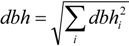
2.1. Plot Network Design
2.2. Plot Measurement Protocols: Nondestructive Measurements
2.2.1. Stems < 10 cm dbh in the 1.5-m Radius Subplot

2.2.2. Stems ≥ 10 cm and < 60 cm dbh in the 20 × 20-m Plot
2.2.3. Stems ≥ 60 cm dbh in the 20-m Horizontal Radius Plot
2.3. Destructive Sampling for Aboveground Biomass and Increment Analysis
2.3.1. Aboveground Biomass
2.3.2. Basal Disc Sampling for Increment Analysis and Age Determination
2.3.3. Sample Processing
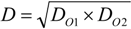
2.4. Intermediate Calculations
2.5. Calculation of Carbon Stocks per Plot in 2012

| Common Name | Estimate aspecies | SE |
|---|---|---|
| rangiora | 141 | 39 |
| marble leaf | 166 | 64 |
| Coprosma areolata | 137 | 48 |
| Coprosma propinqua | 478 | 171 |
| Coprosma rhamnoides | 229 | 30 |
| Spanish heather | 132 | 28 |
| tree fuchsia | 99 | 35 |
| Gaultheria antipoda | 170 | 61 |
| hangehange | 88 | 31 |
| broadleaf | 178 | 47 |
| Hebe traversii | 259 | 95 |
| kanuka | 174 | 26 |
| prickly mingimingi | 313 | 112 |
| manuka | 220 | 30 |
| mingimingi | 228 | 45 |
| kawakawa | 70 | 25 |
| mahoe | 147 | 43 |
| tauhinu | 207 | 39 |
| Douglas-fir | 150 | 53 |
| gorse | 165 | 29 |
| kamahi | 114 | 41 |
| Average species effect | 184 | |
| Estimated b | 0.837 | 0.029 |
| R2 | 0.92 |
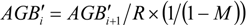
2.6. Calculations of Carbon Stocks per Plot Annually Back to 1990
 is calculated using:
2.7. Plot Age Determination
2.8. National Average Carbon Stocks by Year and Stock Change Estimates
3. Results
3.1. Plot Description
| Plot | Vegetation Type | Elev. (m) | Age (year) | ||||
|---|---|---|---|---|---|---|---|
| Mean | Min | Max | Wtd. Mean | Thresh. Age | |||
| 1 | gorse | 663 | 12.9 | 7.6 | 21.8 | 15.7 | 11 |
| 2 | manuka/kanuka | 373 | 24.2 | 4.1 | 65.5 | 33.4 | 22 |
| 3 | kanuka/wilding conifers | 880 | 12.3 | 1.0 | 30.9 | 10.4 | 8 |
| 4 | kanuka | 623 | 60.7 | 17.6 | 182.0 | 68.8 | 22 |
| 5 | manuka/kanuka | 1240 | 34.6 | 8.3 | 56.4 | 43.7 | 22 |
| 6 | manuka/wilding conifers | 390 | 10.9 | 4.0 | 115.2 | 25.4 | 9 |
| 7 | tauhinu/Coprosma sp. | 105 | 9.4 | 1.0 | 26.0 | 13.2 | 10 |
| 8 | manuka | 260 | 10.6 | 7.7 | 14.0 | 11.9 | 8 |
| 9 | mixed broadleaf /tree ferns | 250 | 28.3 | 8.1 | 47.6 | 34.3 | 15 |
| 10 | manuka/kanuka | 100 | 14.5 | 9.0 | 27.4 | 19.0 | 14 |
| 11 | gorse/manuka/kanuka | 200 | 17.1 | 6.2 | 38.3 | 22.9 | 16 |
| 12 | mixed broadleaf | 180 | 11.6 | 2.5 | 15.3 | 12.9 | 9 |
| 13 | manuka | 190 | 10.8 | 2.5 | 19.2 | 12.1 | 4 |
| 14 | manuka/kanuka | 365 | 14.5 | 5.6 | 25.6 | 17.8 | 11 |
| 15 | mixed broadleaf/manuka | 719 | 18.4 | 1.0 | 26.1 | 15.6 | 15 |
| 16 | mixed broadleaf | 725 | 15.4 | 8.7 | 30.9 | 22.1 | 16 |
| 17 | kanuka | 300 | 25.0 | 12.0 | 52.6 | 31.7 | 22 |
| 18 | manuka/mixed broadleaf/tree ferns | 50 | 8.6 | 4.1 | 17.0 | 10.3 | 9 |
| 19 | manuka/kanuka | 227 | 14.1 | 2.2 | 77.7 | 29.6 | 22 |
| 20 | manuka/kanuka | 160 | 14.9 | 2.0 | 43.9 | 28.1 | 17 |
| mean of measured plots | 18.4 | 5.8 | 46.7 | 23.9 | 14.1 | ||
3.2. Aboveground Carbon Stocks by Species and Assessment Plot Type
3.3. Carbon Stocks in Live and Dead Pools by Assessment Plot Type
| Common Name | AGB Carbon | Plot Assessment Type | ||
|---|---|---|---|---|
| 1.5-m Radius Subplots (dbh < 10 cm) | 20 × 20-m Plot (dbh ≥ 10 cm) | 20-m Radius Plot (dbh ≥ 60 cm) | ||
| manuka | 7.04 | 6.61 | 0.43 | 0.00 |
| kanuka | 6.40 | 3.44 | 2.96 | 0.00 |
| gorse | 2.03 | 2.03 | 0.00 | 0.00 |
| mahoe | 1.07 | 0.86 | 0.21 | 0.00 |
| tauhinu | 0.92 | 0.92 | 0.00 | 0.00 |
| radiata pine | 0.79 | 0.00 | 0.24 | 0.55 |
| mingimingi | 0.56 | 0.54 | 0.02 | 0.00 |
| Douglas-fir | 0.40 | 0.20 | 0.20 | 0.00 |
| Coprosma propinqua | 0.31 | 0.31 | 0.00 | 0.00 |
| broadleaf | 0.28 | 0.28 | 0.00 | 0.00 |
| marble leaf | 0.21 | 0.12 | 0.10 | 0.00 |
| lancewood | 0.20 | 0.03 | 0.17 | 0.00 |
| Spanish heather | 0.19 | 0.19 | 0.00 | 0.00 |
| Coprosma rhamnoides | 0.17 | 0.17 | 0.00 | 0.00 |
| prickly mingimingi | 0.16 | 0.16 | 0.00 | 0.00 |
| five finger | 0.14 | 0.00 | 0.14 | 0.00 |
| Hebe traversii | 0.13 | 0.13 | 0.00 | 0.00 |
| kamahi | 0.11 | 0.11 | 0.00 | 0.00 |
| mountain beech | 0.11 | 0.00 | 0.00 | 0.11 |
| silver fern | 0.08 | 0.00 | 0.08 | 0.00 |
| Others | 0.55 | 0.32 | 0.23 | 0.00 |
| Total | 21.84 | 16.40 | 4.78 | 0.66 |
| Plot Assessment Type | Basal Area at 10-cm (m2/ha) | Carbon (t/ha) | |||||
|---|---|---|---|---|---|---|---|
| AGB | BGB | Dead wood | Litter | Total (Excl. pre-1990 Deadwood) | Pre-1990 Deadwood | ||
| 1.5-m radius subplots (dbh < 10 cm) | 24.70 | 16.40 | 4.10 | 0.00 | 1.21 | 21.71 | 0.00 |
| 20 × 20-m plot (dbh ≥ 10 cm) | 5.97 | 4.78 | 1.20 | 0.23 | 0.00 | 6.21 | 1.29 |
| 20 m-radius plot (dbh ≥ 60 cm) | 0.59 | 0.66 | 0.16 | 0.00 | 0.00 | 0.82 | 0.00 |
| All | 31.26 | 21.84 | 5.46 | 0.23 | 1.21 | 28.73 | 1.29 |
| SE | 3.84 | 2.68 | 0.67 | 0.11 | 0.29 | 3.41 | 0.83 |
| 95% CI | 8.04 | 5.60 | 1.40 | 0.22 | 0.61 | 7.14 | 1.74 |
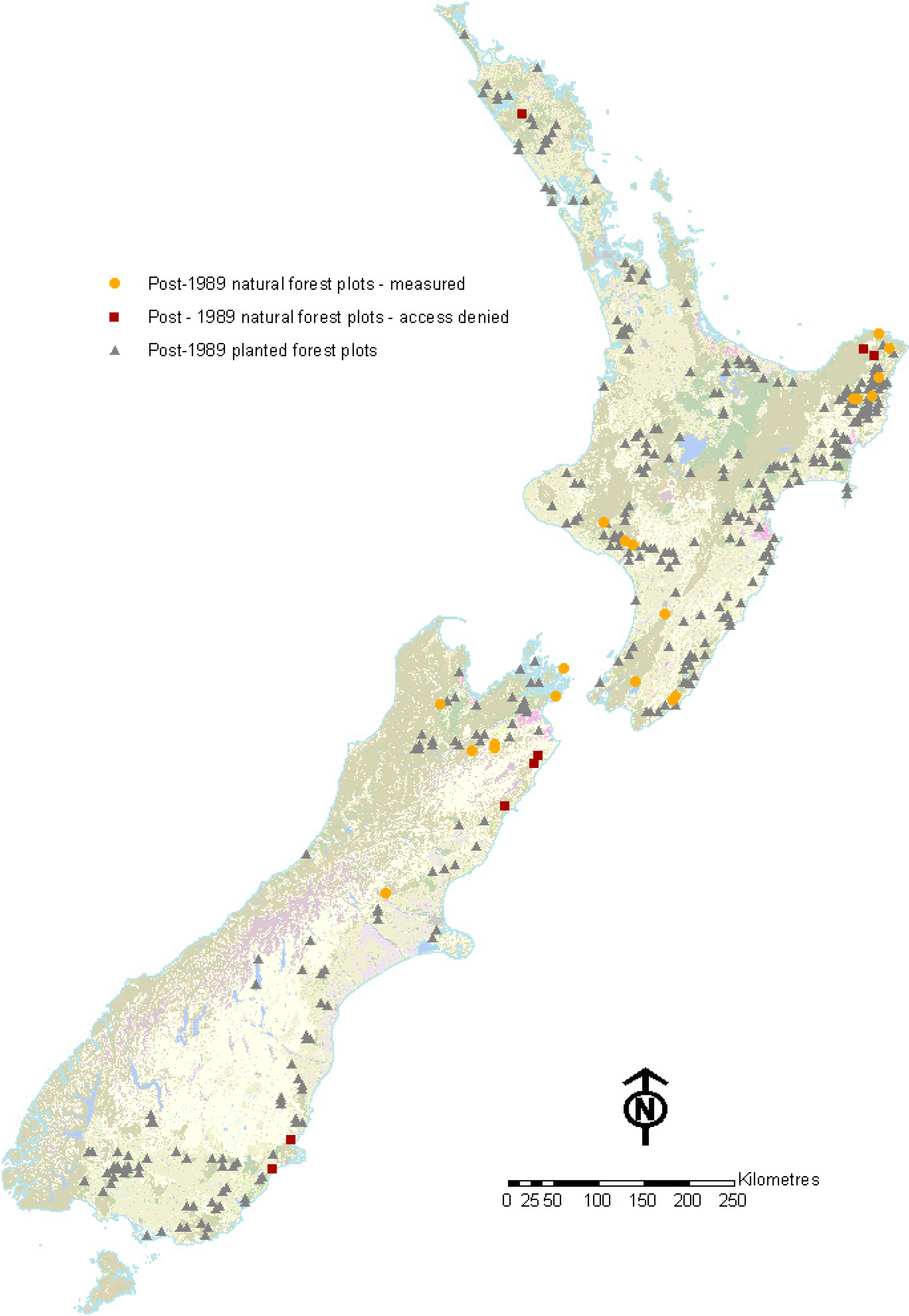
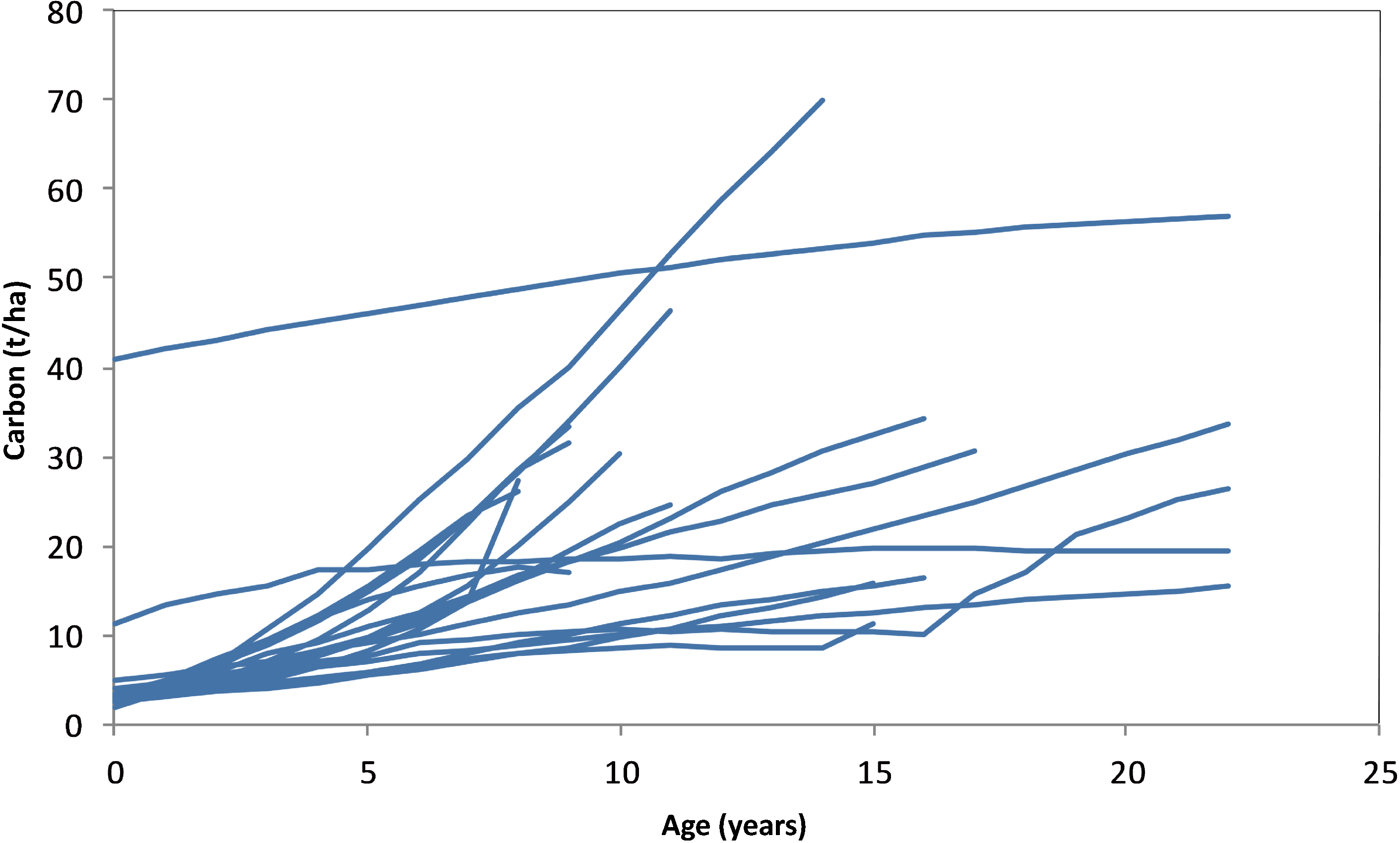
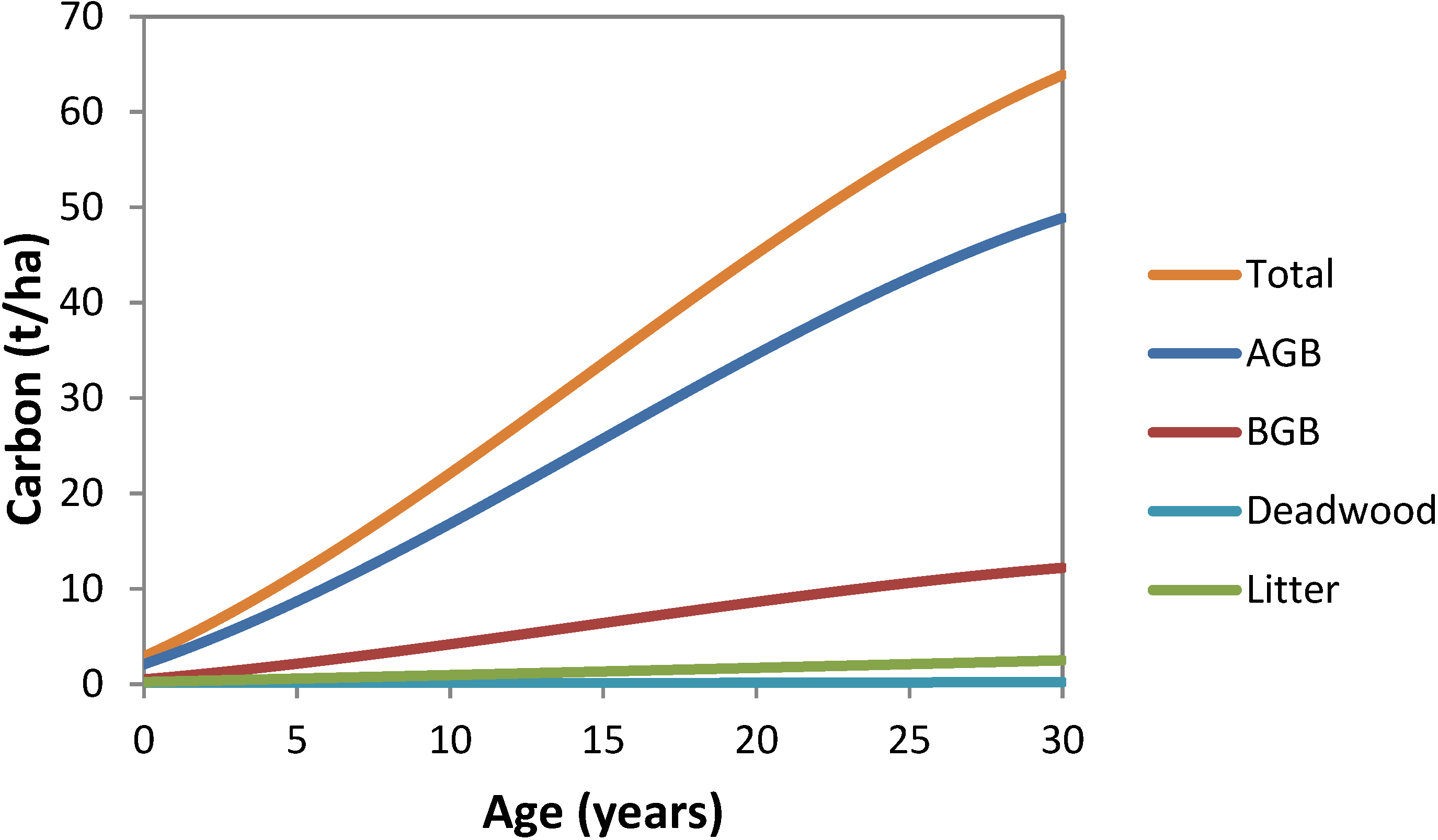
3.4. Carbon Stocks per Plot by Age

3.5. Carbon Stocks and Changes over CP1 of the Kyoto Protocol
| Plot | Carbon (t C/ha) | |||
|---|---|---|---|---|
| 2012 | 2008 | 2008–2012 | 1990 | |
| 1 | 46.46 | 18.60 | 27.86 | 0.00 |
| 2 | 26.31 | 14.61 | 11.70 | 3.13 |
| 3 | 27.44 | 4.94 | 22.50 | 0.00 |
| 4 | 56.98 | 55.15 | 1.83 | 39.88 |
| 5 | 15.43 | 13.35 | 2.07 | 3.58 |
| 6 | 33.36 | 9.36 | 24.00 | 0.00 |
| 7 | 30.44 | 9.87 | 20.57 | 0.00 |
| 8 | 26.25 | 9.61 | 16.64 | 0.00 |
| 9 | 15.81 | 9.72 | 6.09 | 0.23 |
| 10 | 69.91 | 39.92 | 29.99 | 0.00 |
| 11 | 34.23 | 23.11 | 11.11 | 0.02 |
| 12 | 31.70 | 11.94 | 19.76 | 0.00 |
| 13 | 7.06 | 1.69 | 5.38 | 0.00 |
| 14 | 24.63 | 11.88 | 12.75 | 0.00 |
| 15 | 11.35 | 8.49 | 2.86 | 0.10 |
| 16 | 16.46 | 12.30 | 4.16 | 0.67 |
| 17 | 33.76 | 25.01 | 8.75 | 4.21 |
| 18 | 16.91 | 12.01 | 4.90 | 0.00 |
| 19 | 19.56 | 19.61 | −0.05 | 8.93 |
| 20 | 30.63 | 22.84 | 7.78 | 0.00 |
| Mean | 28.73 | 16.70 | 12.03 | 3.04 |
| SE | 3.41 | 2.77 | 2.07 | 2.00 |
| 95% CI | 7.14 | 5.79 | 4.34 | 4.19 |
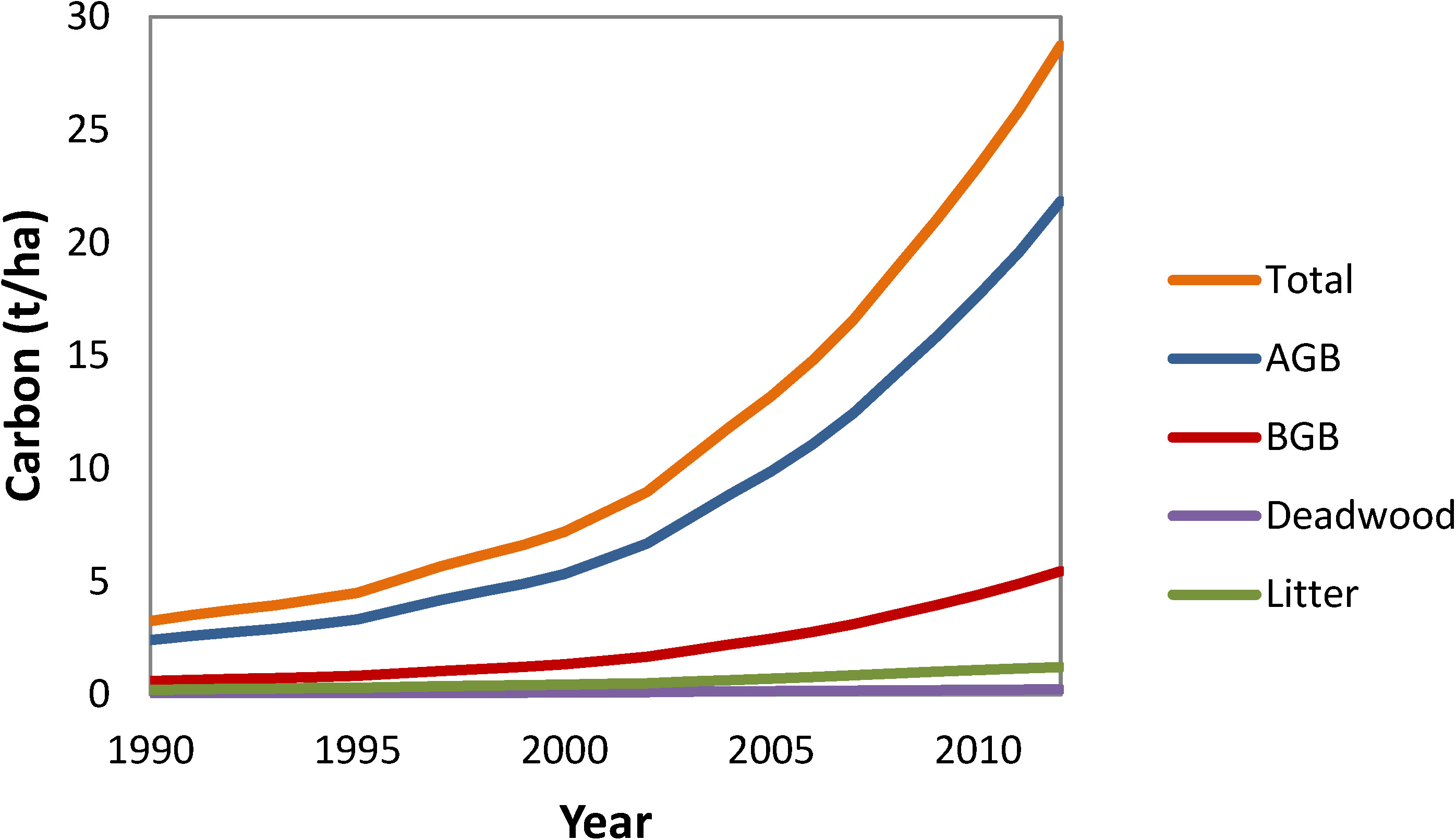
3.6. National Average Carbon Stocks per Hectare by Year and Pool
| Year | Cumulative Number of Post-1989 Forest Plots | % Area Converted to Forest |
|---|---|---|
| 1990 | 5 | 25 |
| 1991 | 5 | 25 |
| 1992 | 5 | 25 |
| 1993 | 5 | 25 |
| 1994 | 5 | 25 |
| 1995 | 6 | 30 |
| 1996 | 8 | 40 |
| 1997 | 10 | 50 |
| 1998 | 11 | 55 |
| 1999 | 11 | 55 |
| 2000 | 11 | 55 |
| 2001 | 13 | 65 |
| 2002 | 14 | 70 |
| 2003 | 17 | 85 |
| 2004 | 19 | 95 |
| 2005 | 19 | 95 |
| 2006 | 19 | 95 |
| 2007 | 20 | 100 |


4. Discussion
4.1. Basal Disc Diameter Increment and Aging
4.2. Predicting Stock Changes by Backcasting from 2012 Inventory Data
4.3. National Carbon Stocks
5. Conclusions
Acknowledgments
Author Contributions
Conflicts of Interest
References
- Bouwman, A.F. Exchange of greenhouse gases between terrestrial ecosystems and the atmosphere. In Soils and the Greenhouse Effect; Bouwman, A.F., Ed.; John Wiley and Sons: New York, NY, USA, 1990; pp. 61–127. [Google Scholar]
- Silver, W.; Ostertag, R.; Lugo, A. The potential for carbon sequestration through reforestation of abandoned tropical agricultural and pasture lands. Restor. Ecol. 2000, 8, 394–407. [Google Scholar] [CrossRef]
- Canadell, J.G.; Raupach, M.R. Managing forests for climate change mitigation. Science 2008, 320, 1456–1457. [Google Scholar] [CrossRef] [PubMed]
- Brown, S.; Gillespie, A.J.; Lugo, A.E. Biomass estimation methods for tropical forests with applications to forest inventory data. For. Sci. 1989, 35, 881–902. [Google Scholar]
- Trotter, C.; Tate, K.; Scott, N.; Townsend, J.; Wilde, H.; Lambie, S.; Marden, M.; Pinkney, T. Afforestation/reforestation of New Zealand marginal pasture lands by indigenous shrublands: The potential for Kyoto forest sinks. Ann. For. Sci. 2005, 62, 865–871. [Google Scholar] [CrossRef]
- Wardle, P. Vegetation of New Zealand; CUP Archive: Cambridge, UK, 1991. [Google Scholar]
- Carswell, F.; Burrows, L.; Mason, N. Above-Ground Carbon Sequestration by Early-Successional Woody Vegetation; Landcare Research Contract Report: LC0809/083; Department of Conservation: Wellington, New Zealand, 2009. [Google Scholar]
- New Zealand’s Greenhouse Gas Inventory 1990–2012; Ministry for the Environment: Wellington, New Zealand, 2014.
- IPCC Guidelines for National Greenhouse Gas Inventories; Prepared by the National Greenhouse Gas Inventories Programme; IGES: Tokyo, Japan, 2006.
- Beets, P.; Brandon, A.; Goulding, C.; Kimberley, M.; Paul, T.; Searles, N. The inventory of carbon stock in New Zealand’s post-1989 planted forest for reporting under the Kyoto protocol. For. Ecol. Manag. 2011, 262, 1119–1130. [Google Scholar] [CrossRef]
- Coomes, D.A.; Allen, R.B.; Scott, N.A.; Goulding, C.; Beets, P. Designing systems to monitor carbon stocks in forests and shrublands. For. Ecol. Manag. 2002, 164, 89–108. [Google Scholar] [CrossRef]
- Navarro Cerrillo, R.M.; Blanco Oyonarte, P. Estimation of above-ground biomass in shrubland ecosystems of southern Spain. For. Syst. 2008, 15, 197–207. [Google Scholar]
- Whittaker, R.H.; Woodwell, G.M. Dimension and production relations of trees and shrubs in the Brookhaven Forest, New York. J. Ecol. 1968, 56, 1–25. [Google Scholar] [CrossRef]
- Whittaker, R.H. Estimation of net primary production of forest and shrub communities. Ecology 1961, 42, 177–180. [Google Scholar] [CrossRef]
- Beets, P.N.; Kimberley, M.O.; Oliver, G.R.; Pearce, S.H. The application of stem analysis methods to estimate carbon sequestration in arboreal shrubs from a single measurement of field plots. Forests 2014, 5, 919–935. [Google Scholar] [CrossRef]
- Dymond, J.R.; Shepherd, J.D.; Newsome, P.F.; Gapare, N.; Burgess, D.W.; Watt, P. Remote sensing of land-use change for Kyoto Protocol reporting: The New Zealand case. Environ. Sci. Policy 2012, 16, 1–8. [Google Scholar]
- Van Breugel, M.; Ransijn, J.; Craven, D.; Bongers, F.; Hall, J.S. Estimating carbon stock in secondary forests: Decisions and uncertainties associated with allometric biomass models. For. Ecol. Manag. 2011, 262, 1648–1657. [Google Scholar]
- Beets, P.N.; Kimberley, M.O.; Oliver, G.R.; Pearce, S.H.; Graham, J.D.; Brandon, A. Allometric Equations for Estimating Carbon Stocks in Natural Forest in New Zealand. Forests 2012, 3, 818–839. [Google Scholar] [CrossRef]
- McCullagh, P.; Nelder, J.A. Generalized Linear Models (Monographs on Statistics and Applied Probability 37); Chapman Hall: London, UK, 1989. [Google Scholar]
- Beets, P.N.; Hood, I.A.; Kimberley, M.O.; Oliver, G.R.; Pearce, S.H.; Gardner, J.F. Coarse woody debris decay rates for seven indigenous tree species in the central North Island of New Zealand. For. Ecol. Manag. 2008, 256, 548–557. [Google Scholar] [CrossRef]
- Kimberley, M.; Bergin, D.; Beets, P. Carbon sequestration by planted native trees and shrubs. In Planting and Managing Native Trees: Technical Handbook; (Technical Article No. 10.5); Bergin, D., Ed.; Tane’s Tree Trust: Rotorua, New Zealand, 2011. [Google Scholar]
- Scott, N.A.; White, J.D.; Townsend, J.A.; Whitehead, D.; Leathwick, J.R.; Hall, G.M.; Marden, M.; Rogers, G.N.; Watson, A.J.; Whaley, P.T. Carbon and nitrogen distribution and accumulation in a New Zealand scrubland ecosystem. Can. J. For. Res. 2000, 30, 1246–1255. [Google Scholar] [CrossRef]
- Litton, C.M.; Boone Kauffman, J. Allometric models for predicting aboveground biomass in two widespread woody plants in Hawaii. Biotropica 2008, 40, 313–320. [Google Scholar] [CrossRef]
- Spurr, S.H. Forest Inventory; Ronald Press: Nova York, NY, USA, 1952; p. 476. [Google Scholar]
- Montagnini, F.; Nair, P. Carbon sequestration: An underexploited environmental benefit of agroforestry systems. Agrofor. Syst. 2004, 61, 281–295. [Google Scholar]
© 2014 by the authors; licensee MDPI, Basel, Switzerland. This article is an open access article distributed under the terms and conditions of the Creative Commons Attribution license (http://creativecommons.org/licenses/by/3.0/).
Share and Cite
Beets, P.N.; Kimberley, M.O.; Paul, T.S.H.; Oliver, G.R.; Pearce, S.H.; Buswell, J.M. The Inventory of Carbon Stocks in New Zealand’s Post-1989 Natural Forest for Reporting under the Kyoto Protocol. Forests 2014, 5, 2230-2252. https://doi.org/10.3390/f5092230
Beets PN, Kimberley MO, Paul TSH, Oliver GR, Pearce SH, Buswell JM. The Inventory of Carbon Stocks in New Zealand’s Post-1989 Natural Forest for Reporting under the Kyoto Protocol. Forests. 2014; 5(9):2230-2252. https://doi.org/10.3390/f5092230
Chicago/Turabian StyleBeets, Peter N., Mark O. Kimberley, Thomas S. H. Paul, Graeme R. Oliver, Stephen H. Pearce, and Joanna M. Buswell. 2014. "The Inventory of Carbon Stocks in New Zealand’s Post-1989 Natural Forest for Reporting under the Kyoto Protocol" Forests 5, no. 9: 2230-2252. https://doi.org/10.3390/f5092230
APA StyleBeets, P. N., Kimberley, M. O., Paul, T. S. H., Oliver, G. R., Pearce, S. H., & Buswell, J. M. (2014). The Inventory of Carbon Stocks in New Zealand’s Post-1989 Natural Forest for Reporting under the Kyoto Protocol. Forests, 5(9), 2230-2252. https://doi.org/10.3390/f5092230