Correlating the Horizontal and Vertical Distribution of LiDAR Point Clouds with Components of Biomass in a Picea crassifolia Forest


Abstract
:1. Introduction
2. Experimental Section
2.1. Study Sites

2.2. LiDAR Data
2.3. Field Measurement

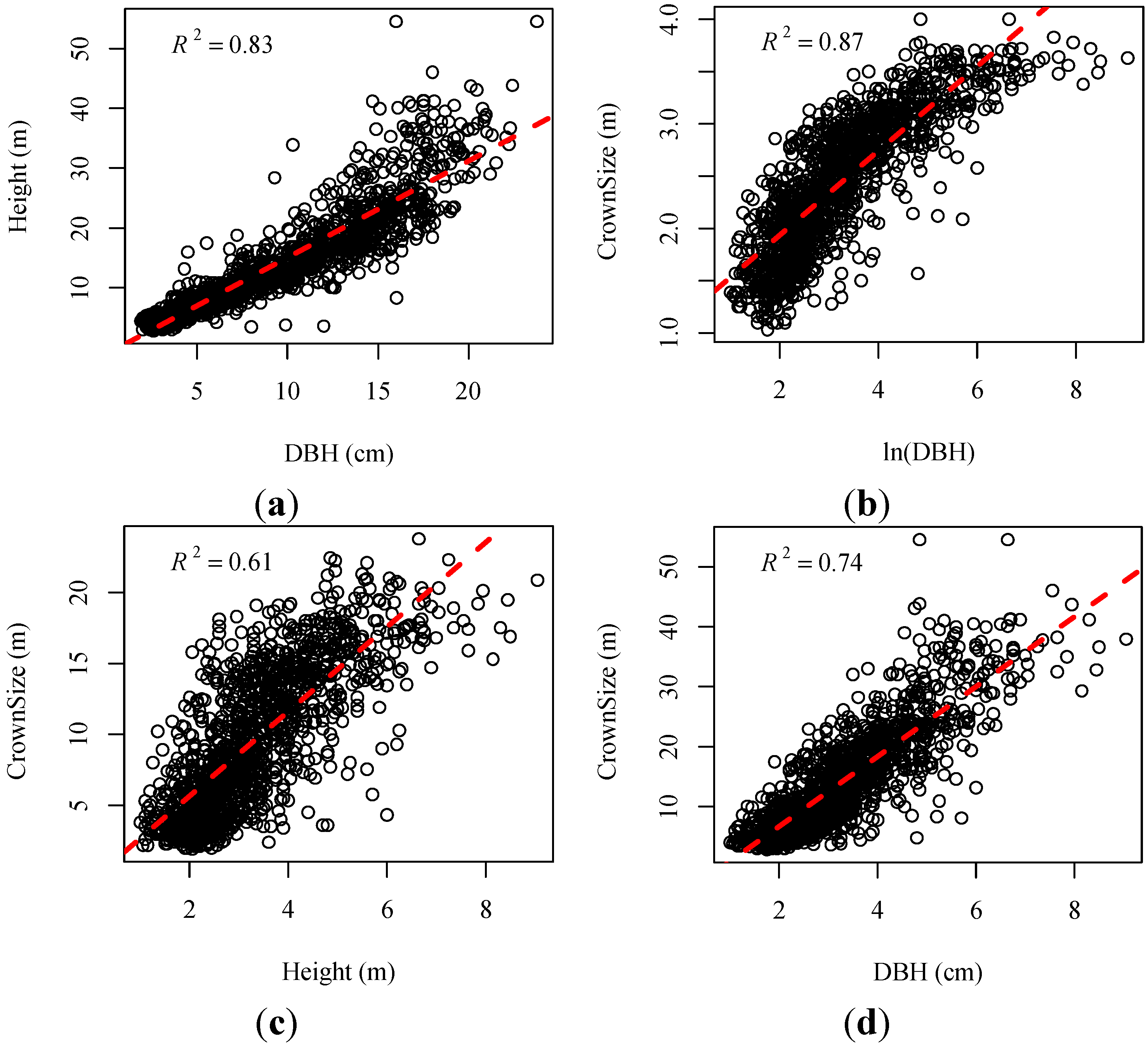
| Dependent Variables (y) | Equation | R2 | Root Mean Squared Error (RMSE) (m) |
|---|---|---|---|
| Height | y = 0.5171 × DBH + 2.1268 | 0.83 | 1.24 |
| Crown Size | y = 7.3496 × ln(DBH) − 8.581 | 0.87 | 1.18 |
| y = 0.2014 × Height + 1.3742 | 0.61 | 0.77 | |
| y = 0.1264 × DBH + 1.4894 | 0.74 | 0.71 |

2.4. Biomass Calculation
2.5. Processing of LiDAR Data
2.6. Individual Tree Identification
2.7. LiDAR Metrics Calculation
yshift_i = yi × a + b
2.8. Vertical Biomass Profile Derivation
3. Results and Discussion
3.1. Individual Tree Identification

| Subplot | Total Segments | Matched Segments | Mismatched Segments | Field Measured | Percentage (%) |
|---|---|---|---|---|---|
| 1 | 53 | 38 | 15 | 98 | 38.78 |
| 2 | 63 | 46 | 17 | 114 | 40.35 |
| 3 | 29 | 22 | 7 | 77 | 28.57 |
| 4 | 54 | 39 | 15 | 80 | 48.75 |
| 5 | 50 | 38 | 12 | 70 | 54.29 |
| 6 | 31 | 24 | 7 | 91 | 26.37 |
| 7 | 68 | 55 | 13 | 120 | 45.83 |
| 8 | 92 | 75 | 17 | 156 | 48.08 |
| 9 | 27 | 20 | 7 | 87 | 22.99 |
| 10 | 28 | 20 | 8 | 100 | 20.00 |
| 11 | 55 | 43 | 12 | 111 | 38.74 |
| 12 | 49 | 39 | 10 | 94 | 41.49 |
| 13 | 38 | 27 | 11 | 62 | 43.55 |
| 14 | 45 | 33 | 12 | 94 | 35.11 |
| 15 | 37 | 28 | 9 | 77 | 36.36 |
| 16 | 18 | 14 | 4 | 37 | 37.84 |
| Total | 737 | 561 | 176 | 1,468 | 38.22 |
| StatisticsError | X (m) | Y (m) | H (m) | D (m) |
|---|---|---|---|---|
| Mean (abs) | 0.28 | 0.30 | 1.02 | 0.46 |
| SD (abs) | 0.38 | 0.41 | 1.19 | 0.53 |
| Number of Trees | 561 (38.22%) | |||
3.2. Correlating Horizontal Variation of Point Clouds with Biomass
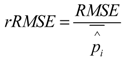
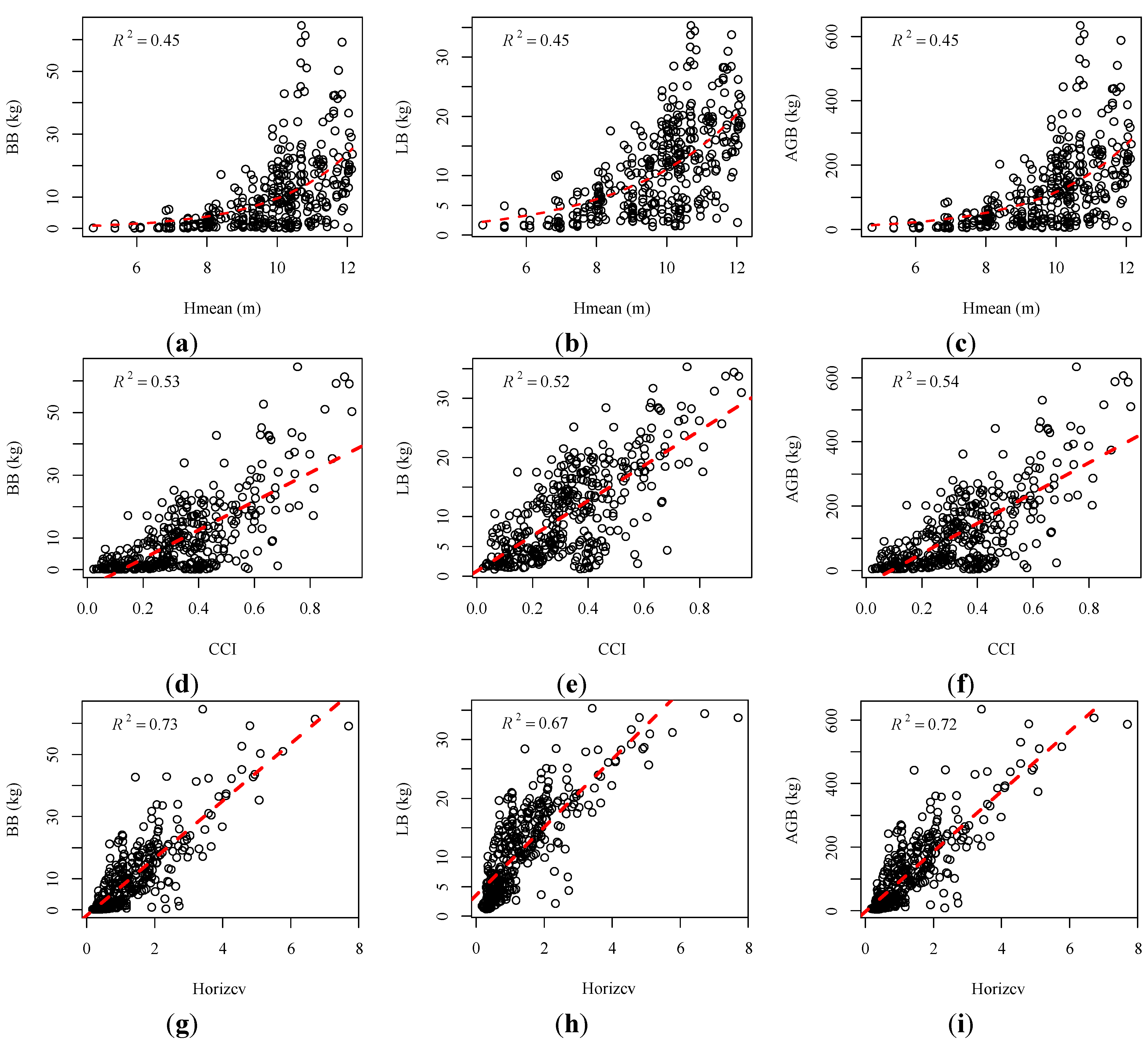
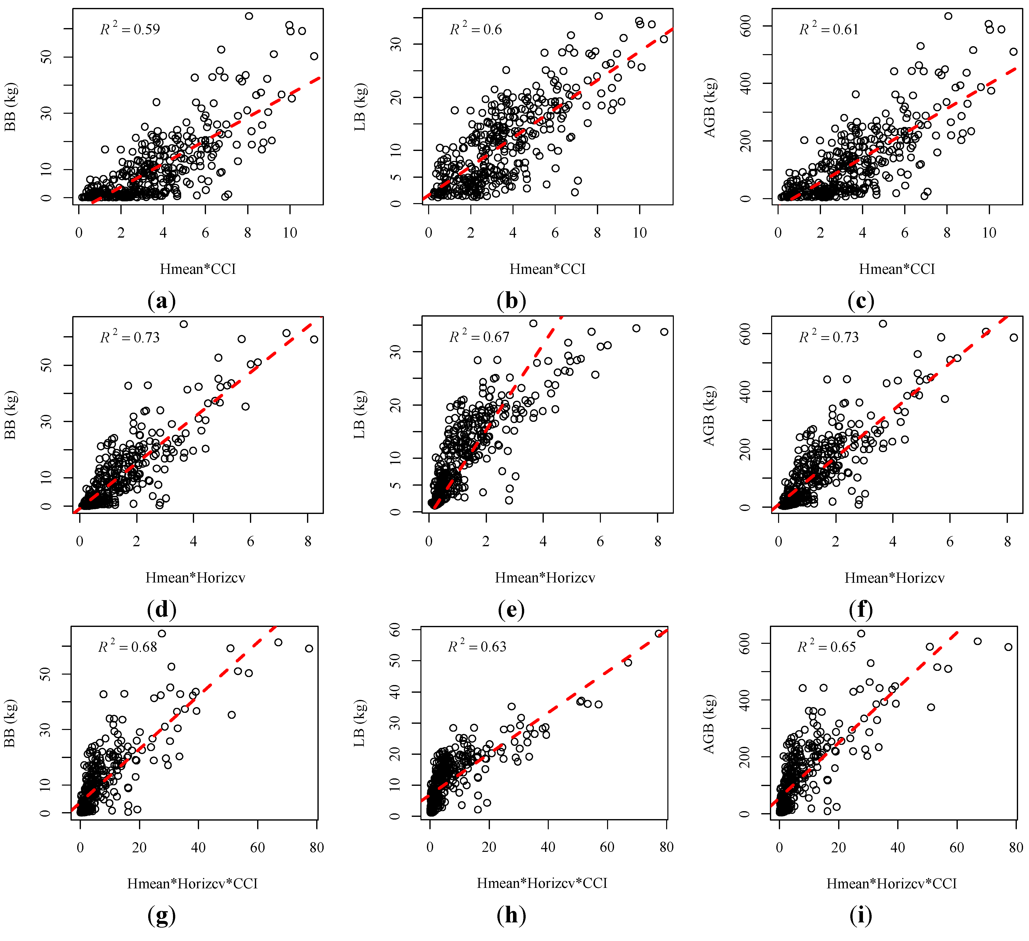
 is the predicted value. The value of RMSE is related to the magnitude of the observed variables. Therefore, we also selected rRMSE, a relative value, to compare the performance of different regression models [18]. A lower rRMSE value often indicates a better regression performance. We first explored the relationships between the conventional height metrics and branch biomass (BB), leaf biomass (LB) and aboveground biomass (AGB) at the individual tree level, respectively. Results (Figure 5a–c) show that biomass for each component of individual trees initially increases with the increasing mean point heights (Hmean) and is saturated when Hmean continues increasing. This means that when the tree height is comparably low, tree height contributes greatly to the amount of biomass. Whereas when tree heights reach a certain height, the canopy increases the speed of growth in the horizontal direction, which also increases the canopy biomass (branch and leaf). Therefore, the horizontal distribution of branches and leaves directly affects the amount of canopy biomass. High correlations were found between the new metric (Horizcv) and the biomass components with high R2 and low RMSE and rRMSE, as shown in Figure 5 and Table 4. Horizcv and AGB for the tree show a good relationship with R2 equal to 0.72, but a higher rRMSE (0.53) than that of BB (0.36) and LB (0.40). Specifically, a higher value of Horizcv means more dispersion of the LiDAR points in the horizontal XY plane. Since branches and leaves rarely grow in only one direction, a greater dispersion probably reflects a wider horizontal distance between the branch and leaf growth and a larger weight of canopy components. Combined metrics were developed by combining the horizontal metrics (CCI and Horizcv) with the vertical metric (Hmean). Both CCI and Horizcv can give an insight into the horizontal distribution of point clouds. Correlations were improved when using the combined metrics (Hmean*CCI and Horizcv*CCI) compared to when using the single metric alone, as shown in Table 4 and Figure 6a–f. The RMSEs and rRMSEs also decreased. Although improvements for the combined metric Horizcv*CCI is smaller than that of Hmean*CCI, the regression models for Horizcv*CCI obtained higher R2 and lower RMSEs and rRMSEs. This is due to the high correlation between Horizcv and the biomass components. However, no significant improvements were obtained when combining Hmean, Horizcv and CCI, as shown in Table 4.
 | Tree | Metrics | Regression Equations | R2 | RMSE | rRMSE |
|---|---|---|---|---|---|
| BB | Hmean | y = 0.0054e0.6842x | 0.45 | 9.78 | 0.97 |
| CCI | y = 45.674x − 5.7033 | 0.53 | 8.02 | 0.81 | |
| Hmean*CCI | y = 4.114x − 4.3411 | 0.59 | 7.47 | 0.76 | |
| Horizcv | y = 69.523x − 0.3626 | 0.73 | 6.11 | 0.36 | |
| Hmean*Horizcv | y = 6.1408x + 0.3972 | 0.73 | 6.07 | 0.59 | |
| Hmean*Horizcv*CCI | y = 0.9624x + 3.7116 | 0.68 | 6.64 | 0.67 | |
| LB | Hmean | y = 0.2487e0.3612x | 0.45 | 5.94 | 0.54 |
| CCI | y = 31.734x + 0.242 | 0.52 | 5.26 | 0.48 | |
| Hmean*CCI | y = 2.8721x + 1.1408 | 0.60 | 4.82 | 0.49 | |
| Horizcv | y = 43.369x + 4.5629 | 0.67 | 4.39 | 0.40 | |
| Hmean*Horizcv | y = 3.8244x + 5.0467 | 0.67 | 4.36 | 0.38 | |
| Hmean*Horizcv*CCI | y = 0.6429x + 6.9487 | 0.63 | 5.14 | 0.52 | |
| AGB | Hmean | y = 0.3638e0.5356x | 0.45 | 98.43 | 0.82 |
| CCI | y = 472.47x − 42.536 | 0.54 | 81.81 | 0.69 | |
| Hmean*CCI | y = 42.693x − 28.919 | 0.61 | 75.65 | 0.64 | |
| Horizcv | y = 711.61x + 13.855 | 0.72 | 63.43 | 0.53 | |
| Hmean*Horizcv | y = 62.835x + 21.663 | 0.72 | 62.86 | 0.50 | |
| Hmean*Horizcv*CCI | y = 9.689x + 56.558 | 0.65 | 71.07 | 0.59 |
| Subplot | Metrics | Regression Equations | R2 | RMSE | rRMSE |
|---|---|---|---|---|---|
| BB | Hmean | y = 101.71x − 426.78 | 0.49 | 178.86 | 0.31 |
| CCI | y = 1,188.4x − 411.79 | 0.35 | 202.00 | 0.35 | |
| Hmean*CCI | y = 74.479x − 44.884 | 0.48 | 179.27 | 0.32 | |
| Horizcv | y = 76.639x +7.0569 | 0.75 | 126.17 | 0.22 | |
| Hmean*Horizcv | y = 6.4054x + 95.374 | 0.84 | 99.76 | 0.18 | |
| Hmean*Horizcv*CCI | y = 6.4395x + 160.2 | 0.83 | 103.42 | 0.18 | |
| LB | Hmean | y = 70.079x − 62.366 | 0.42 | 227.66 | 0.37 |
| CCI | y = 1,034.2x − 229.79 | 0.25 | 223.4 | 0.36 | |
| Hmean*CCI | y = 56.211x + 160.45 | 0.26 | 221.39 | 0.36 | |
| Horizcv | y = 84.016x + 7.792 | 0.84 | 101.92 | 0.16 | |
| Hmean*Horizcv | y = 6.4469x + 147.11 | 0.8 | 114.54 | 0.18 | |
| Hmean*Horizcv*CCI | y = 6.4181x + 216.37 | 0.78 | 122.02 | 0.2 | |
| AGB | Hmean | y = 523.44x − 1,120.8 | 0.65 | 665.19 | 0.17 |
| CCI | y = 6,984.2x − 1,760.1 | 0.6 | 709.83 | 0.18 | |
| Hmean*CCI | y = 404.22x + 672.21 | 0.71 | 597.16 | 0.15 | |
| Horizcv | y = 238.08x + 2,257.8 | 0.36 | 894.31 | 0.22 | |
| Hmean*Horizcv | y = 22.58x + 2,334 | 0.52 | 772.42 | 0.19 | |
| Hmean*Horizcv*CCI | y = 24.377x + 2,456.1 | 0.59 | 712.3 | 0.18 |
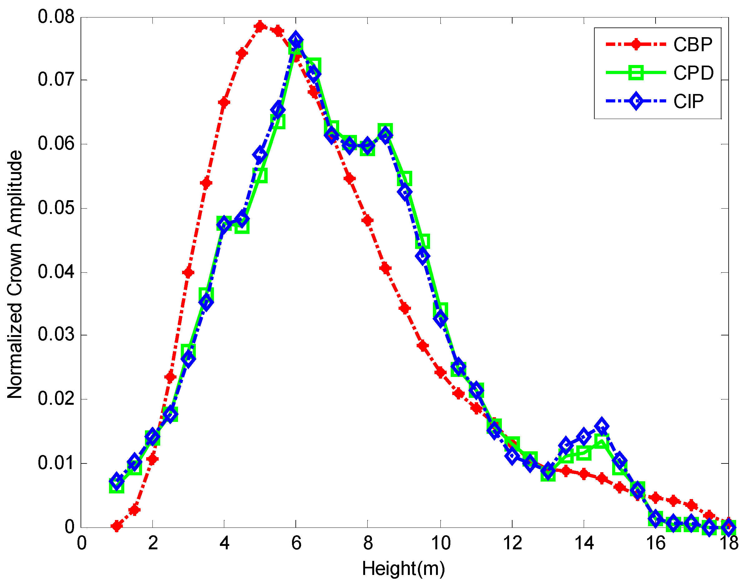
3.3. Correlating Vertical Distribution of Point Clouds with Biomass
| Plot | Pearson’s Correlation Coefficient (R) | Area of Overlap Index (AOI) | ||
|---|---|---|---|---|
| CBP/CPD | CBP/CIP | CBP/CPD | CBP/CIP | |
| S1 | 0.67 | 0.65 | 0.59 | 0.59 |
| S2 | 0.87 | 0.86 | 0.69 | 0.67 |
| S3 | 0.86 | 0.84 | 0.66 | 0.64 |
| S4 | 0.82 | 0.81 | 0.58 | 0.58 |
| S5 | 0.79 | 0.58 | 0.66 | 0.61 |
| S6 | 0.8 | 0.78 | 0.57 | 0.54 |
| S7 | 0.91 | 0.92 | 0.77 | 0.77 |
| S8 | 0.8 | 0.74 | 0.62 | 0.58 |
| S9 | 0.72 | 0.7 | 0.68 | 0.68 |
| S10 | 0.83 | 0.71 | 0.79 | 0.77 |
| S11 | 0.67 | 0.66 | 0.55 | 0.54 |
| S12 | 0.69 | 0.66 | 0.57 | 0.55 |
| S13 | 0.78 | 0.73 | 0.6 | 0.58 |
| S14 | 0.62 | 0.56 | 0.6 | 0.57 |
| S15 | 0.39 | 0.19 | 0.59 | 0.54 |
| L1 | 0.77 | 0.74 | 0.62 | 0.6 |
| L2 | 0.4 | 0.31 | 0.56 | 0.53 |
| L3 | 0.75 | 0.64 | 0.72 | 0.69 |
| L4 | 0.76 | 0.7 | 0.59 | 0.56 |
| L5 | 0.79 | 0.58 | 0.76 | 0.7 |
| L6 | 0.46 | 0.33 | 0.56 | 0.47 |
| L7 | 0.84 | 0.82 | 0.67 | 0.66 |
| L8 | 0.93 | 0.91 | 0.75 | 0.74 |
| L9 | 0.74 | 0.55 | 0.62 | 0.56 |
| L10 | 0.88 | 0.81 | 0.75 | 0.71 |
| L11 | 0.45 | 0.27 | 0.66 | 0.61 |
| L12 | 0.73 | 0.68 | 0.56 | 0.54 |
| L13 | 0.49 | 0.38 | 0.5 | 0.45 |
| L14 | 0.4 | 0.32 | 0.54 | 0.51 |
| L15 | 0.56 | 0.44 | 0.58 | 0.53 |
| L16 | 0.71 | 0.38 | 0.84 | 0.77 |
| L17 | 0.86 | 0.81 | 0.77 | 0.75 |
| L18 | 0.66 | 0.6 | 0.65 | 0.62 |
| L19 | 0.73 | 0.61 | 0.65 | 0.62 |
| L20 | 0.71 | 0.6 | 0.71 | 0.66 |
| Mean | 0.71 | 0.62 | 0.64 | 0.61 |
| SD | 0.15 | 0.19 | 0.08 | 0.09 |

4. Conclusions
Acknowledgments
Author Contributions
Conflicts of Interest
References
- Allouis, T.; Durrieu, S.; Vega, C.; Couteron, P. Stem Volume and Above-Ground Biomass Estimation of Individual Pine Trees From LiDAR Data: Contribution of Full-Waveform Signals. IEEE J. Sel. Top. Appl. Earth Obs. Remote Sens. 2013, 6, 924–934. [Google Scholar] [CrossRef]
- Bortolot, Z.J.; Wynne, R.H. Estimating forest biomass using small footprint LiDAR data: An individual tree-based approach that incorporates training data. ISPRS J. Photogramm. Remote Sens. 2005, 59, 342–360. [Google Scholar] [CrossRef]
- He, Q.-S.; Cao, C.-X.; Chen, E.-X.; Sun, G.-Q.; Ling, F.-L.; Pang, Y.; Zhang, H.; Ni, W.-J.; Xu, M.; Li, Z.-Y.; et al. Forest stand biomass estimation using ALOS PALSAR data based on LiDAR-derived prior knowledge in the Qilian Mountain, western China. Int. J. Remote Sens. 2012, 33, 710–729. [Google Scholar] [CrossRef]
- Drake, J.B.; Dubayah, R.O.; Clark, D.B.; Knox, R.G.; Blair, J.B.; Hofton, M.A.; Chazdon, R.L.; Weishampel, J.F.; Prince, S.D. Estimation of tropical forest structural characteristics using large-footprint lidar. Remote Sens. Environ. 2002, 79, 305–319. [Google Scholar] [CrossRef]
- Drake, J.B.; Dubayah, R.O.; Knox, R.G.; Clark, D.B.; Blair, J.B. Sensitivity of large-footprint lidar to canopy structure and biomass in a neotropical rainforest. Remote Sens. Environ. 2002, 81, 378–392. [Google Scholar] [CrossRef]
- Clark, M.L.; Roberts, D.A.; Ewel, J.J.; Clark, D.B. Estimation of tropical rain forest aboveground biomass with small-footprint lidar and hyperspectral sensors. Remote Sens. Environ. 2011, 115, 2931–2942. [Google Scholar] [CrossRef]
- Lefsky, M.A.; Cohen, W.B.; Harding, D.J.; Parker, G.G.; Acker, S.A.; Gower, S.T. Lidar remote sensing of above-ground biomass in three biomes. Glob. Ecol. Biogeogr. 2002, 11, 393–399. [Google Scholar] [CrossRef]
- Ahmed, R.; Siqueira, P.; Hensley, S. A study of forest biomass estimates from lidar in the northern temperate forests of New England. Remote Sens. Environ. 2013, 130, 121–135. [Google Scholar] [CrossRef]
- Huang, W.; Sun, G.; Dubayah, R.; Cook, B.; Montesano, P.; Ni, W.; Zhang, Z. Mapping biomass change after forest disturbance: Applying LiDAR footprint-derived models at key map scales. Remote Sens. Environ. 2013, 134, 319–332. [Google Scholar] [CrossRef]
- Næsset, E.; Bollandsås, O.M.; Gobakken, T.; Gregoire, T.G.; Ståhl, G. Model-assisted estimation of change in forest biomass over an 11year period in a sample survey supported by airborne LiDAR: A case study with post-stratification to provide “activity data”. Remote Sens. Environ. 2013, 128, 299–314. [Google Scholar] [CrossRef]
- Ni-Meister, W.; Lee, S.; Strahler, A.H.; Woodcock, C.E.; Schaaf, C.; Yao, T.; Ranson, K.J.; Sun, G.; Blair, J.B. Assessing general relationships between aboveground biomass and vegetation structure parameters for improved carbon estimate from lidar remote sensing. J. Geophys. Res. 2010, 115. [Google Scholar]
- Popescu, S.C. Estimating biomass of individual pine trees using airborne lidar. Biomass. Bioenerg. 2007, 31, 646–655. [Google Scholar] [CrossRef]
- Zhao, K.; Popescu, S.; Nelson, R. Lidar remote sensing of forest biomass: A scale-invariant estimation approach using airborne lasers. Remote Sens Environ. 2009, 113, 182–196. [Google Scholar] [CrossRef]
- Popescu, S.C.; Wynne, R.H.; Nelson, R.F. Estimating plot-level tree heights with lidar: Local filtering with a canopy-height based variable window size. Comput. Electron. Agrc. 2002, 37, 71–95. [Google Scholar] [CrossRef]
- Barraud, J. The use of watershed segmentation and GIS software for textural analysis of thin sections. J. Volcanol. Geoth. Res. 2006, 154, 17–33. [Google Scholar] [CrossRef]
- Andersen, H.-E.; McGaughey, R.J.; Reutebuch, S.E. Estimating forest canopy fuel parameters using LIDAR data. Remote Sens. Environ. 2005, 94, 441–449. [Google Scholar] [CrossRef]
- Scott, J.H.R.; Elizabeth, D. Assessing Crown Fire Potential by Linking Models of Surface and Crown Fire Behavior. Res. Pap. RMRS-RP-29; U.S. Department of Agriculture, Forest Service, Rocky Mountain Research Station: Fort Collins, CO, USA, 2001; p. 59. [Google Scholar]
- Pang, Y.; Li, Z.-Y. Inversion of biomass components of the temperate forest using airborne Lidar technology in Xiaoxing’an Mountains, Northeastern of China. Chin. J. Plant Ecol. 2013, 36, 1095–1105. [Google Scholar] [CrossRef]
- He, Q.; Chen, E.; An, R.; Li, Y. Above-Ground Biomass and Biomass Components Estimation Using LiDAR Data in a Coniferous Forest. Forests 2013, 4, 984–1002. [Google Scholar] [CrossRef]
- Tian, X.; Su, Z.; Chen, E.; Li, Z.; van der Tol, C.; Guo, J.; He, Q. Estimation of forest above-ground biomass using multi-parameter remote sensing data over a cold and arid area. Int. J. Appl. Earth Observ. Geoinf. 2012, 14, 160–168. [Google Scholar] [CrossRef]
- Li, X.; Li, X.; Li, Z.; Ma, M.; Wang, J.; Xiao, Q.; Liu, Q.; Che, T.; Chen, E.; Yan, G.; et al. Watershed Allied Telemetry Experimental Research. J. Geophys. Res. 2009, 114. [Google Scholar] [CrossRef]
- Cao, C.; Bao, Y.; Xu, M.; Chen, W.; Zhang, H.; He, Q.; Li, Z.; Guo, H.; Li, J.; Li, X.; et al. Retrieval of forest canopy attributes based on a geometric-optical model using airborne LiDAR and optical remote-sensing data. Int. J. Remote Sens. 2012, 33, 692–709. [Google Scholar] [CrossRef]
- Wang, J.Y.; Ju, K.J.; Fu, H.E.; Chang, X.X.; He, H.Y. Study on biomass of water conservation forest on North Slope of Qilian Mountains. J. Fujian Coll. For. 1998, 18, 319–323. [Google Scholar]
- Qin, Y.; Li, B.; Niu, Z.; Huang, W.; Wang, C. Stepwise decomposition and relative radiometric normalization for small footprint LiDAR waveform. China Ser. D 2010, 54, 625–630. [Google Scholar] [CrossRef]
- Vincent, L.; Soille, P. Watersheds on digital spaces-An efficient algorithm based on immersion simulations. IEEE Trans. Patt. Anal. 1991, 13, 583–598. [Google Scholar] [CrossRef]
- Liu, Q.; Li, Z.; Chen, E.; Pang, Y.; Wu, H. Extracting height and crown of individual tree using airborne LIDAR data. J. Beijing For. Univ. 2008, 30, 83–89. [Google Scholar]
- Edson, C.; Wing, M.G. Airborne Light Detection and Ranging (LiDAR) for Individual Tree Stem Location, Height, and Biomass Measurements. Remote Sens. 2011, 3, 2494–2528. [Google Scholar] [CrossRef]
- Li, W.; Niu, Z.; Gao, S.; Qin, Y.C. Analyzing and retrieving structure information of Picea crassifolia based on airborne light detection and ranging data. J. Remote Sens. 2013, 6, 1612–1626. [Google Scholar]
© 2014 by the authors; licensee MDPI, Basel, Switzerland. This article is an open access article distributed under the terms and conditions of the Creative Commons Attribution license (http://creativecommons.org/licenses/by/3.0/).
Share and Cite
Li, W.; Niu, Z.; Gao, S.; Huang, N.; Chen, H. Correlating the Horizontal and Vertical Distribution of LiDAR Point Clouds with Components of Biomass in a Picea crassifolia Forest. Forests 2014, 5, 1910-1930. https://doi.org/10.3390/f5081910
Li W, Niu Z, Gao S, Huang N, Chen H. Correlating the Horizontal and Vertical Distribution of LiDAR Point Clouds with Components of Biomass in a Picea crassifolia Forest. Forests. 2014; 5(8):1910-1930. https://doi.org/10.3390/f5081910
Chicago/Turabian StyleLi, Wang, Zheng Niu, Shuai Gao, Ni Huang, and Hanyue Chen. 2014. "Correlating the Horizontal and Vertical Distribution of LiDAR Point Clouds with Components of Biomass in a Picea crassifolia Forest" Forests 5, no. 8: 1910-1930. https://doi.org/10.3390/f5081910
APA StyleLi, W., Niu, Z., Gao, S., Huang, N., & Chen, H. (2014). Correlating the Horizontal and Vertical Distribution of LiDAR Point Clouds with Components of Biomass in a Picea crassifolia Forest. Forests, 5(8), 1910-1930. https://doi.org/10.3390/f5081910