Article

Wood Density-Climate Relationships Are Mediated by Dominance Class in Black Spruce (Picea mariana (Mill.) B.S.P.)

1
Faculty of Natural Resources Management, Lakehead University, Thunder Bay, ON P7B 5E1, Canada
2
Renewable Materials Research Centre, Université Laval, Sainte-Foy, QC G1V 0A6, Canada
3
Chaire de recherche sur la forêt habitée, Département de Biologie, Chimie et Géographie, Université du Québec à Rimouski, 300 allée des Ursulines, Rimouski, QC G5L 3A1, Canada
*
Author to whom correspondence should be addressed.
Forests 2014, 5(6), 1163-1184; https://doi.org/10.3390/f5061163
Submission received: 28 February 2014 / Revised: 8 May 2014 / Accepted: 20 May 2014 / Published: 28 May 2014

Abstract

:
The relationships between climate and wood density components, i.e., minimum ring density, maximum ring density and mean ring density have been studied mainly in dominant trees. However, the applicability of the findings to trees of other dominance classes is unclear. The aim of this study was to address whether climate differentially influences wood density components among dominance classes. X-ray densitometry data was obtained from 72 black spruce (Picea mariana (Mill.) B.S.P.) trees harvested in Northwestern Ontario, Canada. Dominant, co-dominant and intermediate trees were sampled and the data analysed using mixed-effect modelling techniques. For each density component, models were first fitted to the pooled data using ring width and cambial age as predictors, before monthly climatic variables were integrated into the models. Then, separate models were fitted to the data from each dominance class. In general, the addition of climatic factors led to a small but significant improvement in model performance. The predicted historical trends were well synchronized with the observed data. Our results indicate that trees from all dominance classes in a stand should be sampled in order to fully characterize wood density-climate relationships.

1. Introduction

Over the past several decades, boreal forest biomass production has increased along with increasing mean annual temperatures [1]. As a measure of forest productivity, annual biomass increment has often been estimated by considering the effect of climate on tree ring width [2,3]. In gymnosperms, ring width has been shown to vary with temperature [4,5], water availability [6,7] and the concentration of atmospheric carbon dioxide [8,9]. By necessity, calculations of annual biomass increment must also include wood density, for which constant values are often assumed [10,11]. Since wood density is known to change significantly according to stand conditions, genetics and climate [12], more detailed knowledge of this variability may help to improve biomass estimations [13].
In gymnosperms, anatomical changes throughout the growing season generally lead to a transition from large, thin-walled earlywood tracheids to smaller, thicker-walled latewood tracheids, hence wood density increases across annual rings [14]. These anatomical changes result from variation in cambial activity triggered by crown processes [15,16,17], which are under a degree of climatic control, at least for the onset of growth and dormancy [18,19].
Considering these relationships, a degree of correlation between climate and wood density components is expected in spruce and other temperate or boreal conifer species, e.g., see Bouriaud et al. [20]. Generally, the association between climatic variables and wood density components is stronger for maximum than for minimum or mean ring density [21,22]. As a consequence, maximum density series are frequently used in dendroclimatic studies [23,24]. Such studies typically focus on trees occupying dominant or co-dominant positions in the canopy. However, the response of intermediate trees may also be important, as they represent a significant proportion of the final composition of mature forest stands, and therefore contribute both ecologically and commercially to forest functions [25]. Information from intermediate trees might improve the accuracy of predictions from carbon accounting models. Many previous studies have shown that functional processes change with both tree age and size [26]. The interrelated effects of these variables are difficult to disentangle [27], although recent research suggests that size may be the most important factor [27,28].
In a closed-canopy stand, smaller trees in lower canopy positions are likely to respond differently to climatic factors because of their more restricted access to resources [29]. Little scientific attention has been given to the potential effect of tree dominance on wood density-climate relationships, while the few studies that have studied the relationship between tree growth and climate have reported contrasting results. Dominant trees of silver fir (Abies alba Mill.) and Norway spruce (Picea abies (L.) Karst.) were reported to be more sensitive to climatic variables than trees in lower canopy positions [29,30]. Conversely, De Luis et al. [31] found that growth was more sensitive to climate in small individuals of Pinus halepensis and P. pinea than in larger trees. In lodgepole pine (Pinus contorta Dougl. ex Loud.), Chhin et al. [32] reported a constant growth response to climatic variables across tree sizes.
This study presents an analysis of wood density–climate relationships among different dominance classes in black spruce (Picea mariana (Mill.) B.S.P.). This species constitutes an abundant resource over a vast area of distribution covering the entire North American boreal forest biome. Within-stem ring density variation in this species has been described radially [33,34], longitudinally [35], as a function of growth rate [33], and in various site conditions [36]. Although it is reasonable to hypothesize that black spruce might exhibit some variability in wood density–climate relationships among trees occupying different levels of the canopy, there is currently little information about the exact nature of these interactions. The aims of this study were therefore: (1) to characterize the relationship between climatic factors and minimum, maximum and mean ring density of black spruce from even-aged, closed-canopy stands; and (2) to quantify the variation in wood density–climate relationships among trees occupying three different canopy positions, i.e., dominant, co-dominant and intermediate classes.

2. Materials and Methods

2.1. Sampling and Climate Data

We sampled 13 natural black spruce stands (stand age from 60 to 138) in the Lake St. Joseph Ecoregion, 400 km northwest of Thunder Bay, Ontario, located between 51°42′ N and 52°6′ N and between 90°3′ W and 94°31′ W, at an elevation of 400 m. Each site was pre-selected according to the following criteria: (1) species composition (dominated by black spruce); (2) stand age (>50 years old) and (3) crown closure (>55% crown closure). All stands were of natural origin and had never been managed. The mean length of the growing season was between 162 and 179 days. Further information is available in the Ecoregions Working Group [37] publication. Monthly temperature (mean, minimum and maximum) and precipitation were obtained from the nearest Environment Canada weather station (Sioux Lookout at 50°07′ N, 91°54′ W). A small number of missing meteorological data points was substituted with data from a neighbouring station (Kenora at 49°48′ N, 94°32′ W). Climate data were collected over a period of 94 years, from 1915 until 2008. Over this period, mean annual temperature ranged from −1.8 to 4.3 °C, mean minimum temperature varied between −8.4 and −0.7 °C, and mean maximum temperature between −3.0 and 9.4 °C. Annual precipitation ranged from 393 to 1092 mm, while May to September rainfall was between 141 and 758 mm. From 1915 to 2008, there were increasing trends in both average annual temperature and precipitation (Figure 1).
Three temporary sample plots with a radius of 5.64 m (100 m2) were established at each site, and diameter at breast height (DBH, cm) was measured on all live black spruce trees. From each plot, three trees with no visible signs of damage were harvested: (1) the tree with the largest DBH; (2) the tree with the DBH closest to the quadratic mean DBH of the plot and (3) the tree with the DBH closest to the average of the quadratic mean DBH and that of the smallest tree in the plot, which we will refer to as dominant, co-dominant and intermediate trees, respectively. After felling, the total height of each sample tree was recorded and a 5-cm thick transverse disc was cut at breast height (i.e., 1.3 m above ground level).

2.2. Annual Ring Width and Wood Density Measurements

From each sample disk, a pith-to-bark strip with dimensions of 2 mm in the longitudinal direction and 25 mm tangentially was cut using a twin-blade circular saw. The strips were stored in a conditioning chamber at 60% relative humidity and 20 °C until they reached a constant mass, corresponding to an equilibrium moisture content of 12%. Pith-to-bark density profiles were obtained using a QTRS-01X Tree Ring Analyzer (Quintek Measurement Systems Inc., Knoxville, TN, USA). The samples were scanned in the longitudinal direction with an X-ray beam at a resolution of 40 μm (For details, see [38]). From these measurements, minimum ring density (MnD), maximum ring density (MxD) and mean ring density (RD) were calculated. For explanations of all the abbreviations used in this article, refer to Table 1.
Ring density was highly variable in the juvenile zone [38], but remained relatively constant after a cambial age (CA) of around 25 years. In addition, a density decline close to the bark was detected in some rings older than 60 years. Therefore, to minimize variation in density due to cambial age, only the rings with a CA between 25 and 60 years were included in the subsequent analyses. Furthermore, climatic data for the years prior to 1915 were unavailable for this region, so the rings formed during that period were also omitted. Tree-ring series were cross-dated using the COFECHA software [39]. Some discs, mostly from intermediate trees, contained extremely narrow rings, particularly close to the bark [38]. Since some of these narrow rings (<0.2 mm) cannot be reliably cross-dated, they were also omitted from the analysis. Additionally, 45 entire trees were omitted from the analysis because of damaged or small-diameter (<8 cm) stems. The final dataset therefore consisted of radial samples from 72 trees (30 dominant, 28 co-dominant and 14 intermediate trees), totalling 2455 annual rings. Details of annual ring width (RW) and density components for each dominance class are shown in Table 2.
Figure 1. Mean annual temperature and precipitation (each value was standardized by subtracting the population mean and then dividing by the standard deviation) from 1915 to 2008 in the sampling area. General trends are illustrated using loess smoothing lines.
Forests 05 01163 g001
Table 1. Abbreviations used in this article.
AbbreviationsDescription (unit)
MnDMinimum ring density (kg m−3)
MxDMaximum ring density (kg m−3)
RDRing density (kg m−3)
RWRing width (mm)
CACambial age (years)
Tmean.iMean daily temperature of month i in the current year (°C)
Tmin.iAverage minimum daily temperature of month i in the current year (°C)
Tmax.iAverage maximum daily temperature of month i in the current year (°C)
ExTmax.iExtreme maximum daily temperature of month i in the current year (°C)
Prec.iPrecipitation of month i in the current year (mm)
Prec.i.pPrecipitation of month i in the previous year (mm)
Table 2. Mean (standard deviation) ring-level characteristics for each dominance class.
Dominance ClassTree Age (years)DBH (cm)Height (m)Number of RingsRW (mm)Mean Ring Density (kg/m3)Minimum Ring Density (kg/m3)Maximum Ring Density (kg/m3)
Dominant8419.717.610151.16 (0.48)481.76 (58.59)348.25 (45.51)776.96 (101.44)
Co-dominant8113.314.79680.78 (0.35)529.68 (66.53)384.35 (61.72)784.16 (86.44)
Intermediate7911.514.54720.64 (0.24)535.07 (65.53)396.38 (64.81)750.28 (81.51)

2.3. Data Analysis

A statistical modelling approach was applied to remove the long-term trends in tree-ring series. Such techniques have been shown to produce similar results to those obtained using traditional dendrochronological methods [40]. First, models were developed to describe the variation in MnD, MxD, and RD as functions of RW and CA. The main purpose of this step was to detrend the time series to remove the known effects of ring width and cambial age on wood density. Our results therefore describe, for any ring number from the pith, the additional effects of climatic variables on ring density components, i.e., over and above the well-documented relationship between climate and radial growth.
As the data were longitudinal (i.e., a series of repeated measurements on the same samples), the developed models included both fixed and random effects. Such mixed-effects models account for dependence among observations on the same sample, allowing more accurate estimation of parameter standard errors [41]. Random intercepts were included at the site- and tree-level, without further partitioning the sources of within-group errors for each parameter. A first-order autoregressive (AR1) correlation structure was also included to account for correlation among observations at successive cambial ages [41]. After testing different mathematical transformations of the covariates, the fixed effects for each wood density component (Model 1) were as follows:
Forests 05 01163 i001
where WDi represents MnD, MxD, or RD, fi(CA, RW) a function of CA and RW, and β0, β1, and β2 denote the fixed effects parameters to be estimated.
In a second step, the residuals from each density component model in Equation (1) were correlated to climatic variables. Density components from each annual ring were modelled as functions of monthly climate data from January in the year prior to wood formation to October during the current year. These data were selected because in the study region, cambial activity generally ceases in October [18], while effects carried over from the previous year have also been identified [42,43]. These monthly climatic variables were then introduced into the wood density models (Model 1) to test for any significant effects. The general equation (Model 2) for the fixed effects was therefore expressed as follows:
WDi = fi(CA,RW) + gMi(climate)
where gi(climate) is the effect of a given climate variable on a given density component.
To establish the general form of the fixed effects, models were initially fitted to the pooled dataset before separate models were fitted to data from each dominance class. The residuals for the models were assumed to be normally distributed, with N (0, σi2). Model selection was based on Akaike’s [44] information criterion (AIC) and likelihood ratio tests for nested models. For a given dataset, AIC provides information on the relative adequacy of nested statistical models, and models with lower values were selected. All models were fitted using functions contained in the nlme library [45] of the R statistical programming environment [46]. Because of the large number of candidate explanatory variables, stepwise regression was first used to progressively fit each model with no random effects [47]. Then, random effects were introduced in the best model obtained from the first step. Additionally, coefficients of determination were calculated for each level of the fixed and random effects [48]. The accuracy of the predictions were evaluated using two error statistics, i.e., mean percentage error (ME%) and mean absolute percentage error (|ME|%). The agreement between the predicted and observed chronologies was assessed for their degree of correlation using the Spearman’s rank correlation coefficient, and for their synchronicity using the Gleichläufigkeit statistic, or g-score [49] from the glk function in the DplR library [50].

3. Results

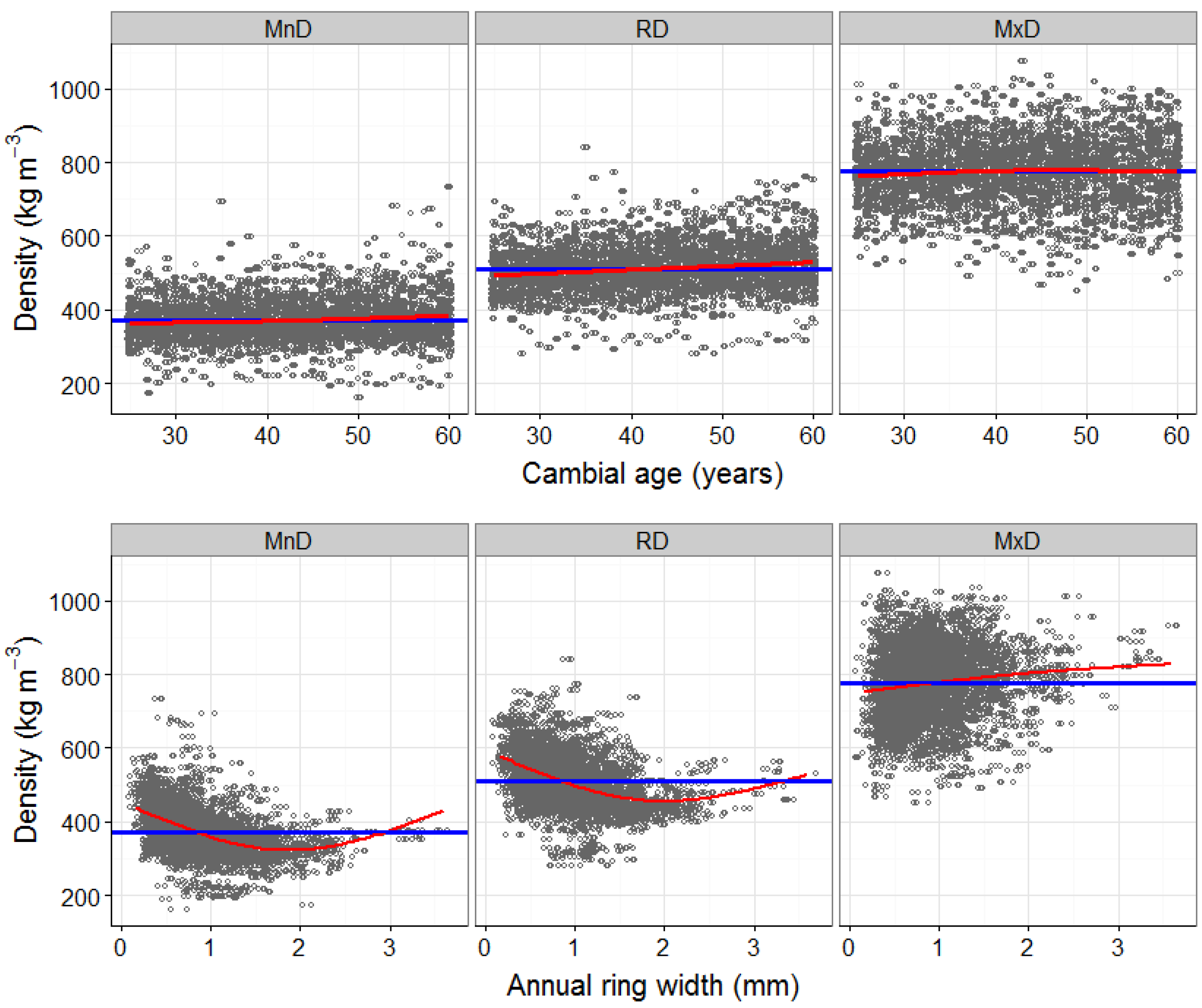
3.1. Detrending the Effects of Cambial Age and Ring Width on Wood Density Components (Model 1)

For each density component, the effects of cambial age varied, and different mathematical forms of ring width were used in the models (Table 3, Table 4 and Table 5). There was a small positive effect of CA on both MxD and RD. Additionally, while annual ring width was negatively related to both MnD and RD, it was positively related to MxD (see appendix Figure A1).
The non-climatic model (Model 1) was generally unbiased for all density components, despite the moderately high |ME|% value (Table 3, Table 4 and Table 5). The highest R2 (calculated from the fixed effects of the models) was 0.22 in the MnD model compared to 0.07 and 0.01 in the RD and MxD models, respectively. For all density components, between-tree differences accounted for most of the random variation in the models, i.e., 41%, 52%, and 51%, for MnD, MxD, and RD, respectively, with only a small random effect of site.

3.2. Inclusion of Climate Variables in the Models (Model 2)

In models fitted to the pooled data, MnD was found to decrease with lower minimum temperatures during May, and increased with lower minimum temperatures in January and July. In addition, precipitation in May, June, and the previous March were negatively related to MnD, while the opposite relationship was found with precipitation in the previous October (Table 3). Temperature in the early growing season (April to June) was positively correlated with MxD. Conversely, extreme high temperatures in August were correlated with lower MxD, while high precipitation levels in July and August and lower rainfall in May of the previous year were associated with lower MxD (Table 4). Mean temperatures in April and May were positively related to RD, while mean temperatures in September, along with the minimum temperatures in January and July were negatively related to RD. Additionally, lower precipitation in June, August of the current year, and in March, August and December of the previous year, were associated with higher RD. However, lower precipitation in April and the previous May were linked with lower RD (Table 5). In general, the inclusion of climatic variables (Model 2) resulted in lower AIC values and improved error statistics (Table 3, Table 4 and Table 5). The climatic variables increased the contribution of the fixed effects to the total variability of MnD, MxD, and RD by 2%, 2%, and 4%, respectively. The increase in both Spearman’s correlation coefficients and g-scores from Model 1 to Model 2 (Table 6) also confirmed that the inclusion of climatic variables was necessary.
The separate versions of model 2 fitted to data from the different dominance classes included different non-climatic variables for each model. For each density component the magnitude of RW and CA differed slightly among the dominance classes (Table 3, Table 4 and Table 5). The effects of climatic variables also varied between dominance classes. The negative relationship between minimum temperature in January and MnD that was found in the pooled data was not detected in intermediate trees, while a positive relationship between the minimum temperature in May and MnD was found across all dominance classes (Table 3). However, the negative effect of July minimum temperature on MnD was not found in co-dominant trees. Furthermore, MnD in intermediate trees was less sensitive to precipitation in the early growing season, although it was negatively related to June precipitation levels. The precipitation during the previous March was significant in the MnD models for the dominant and co-dominant trees only, while the precipitation level in the previous October was significant only for the co-dominant trees (Table 3).
Table 3. Estimated coefficients (Est.) and associated standard error (S.E.) for minimum ring density at different dominance classes.
Minimum DensityPooledDominantCo-dominantIntermediate
Model 1Model 2Model 2Model 2Model 2
Est.S.E.Est.S.E.Est.S.E.Est.S.E.Est.S.E.
(Intercept)277.2 ***7.8291.7 ***10.2302.8 ***14.1273.8 ***14.0291.8 ***21.9
Forests 05 01163 i00281.8 ***4.283.3 ***4.159.5 ***6.684.9 ***6.2100.5 ***9.1
Tmin.1 −0.7 ***0.1−0.7 ***0.2−0.8 **0.3
Tmin.5 2.4 ***0.22.2 ***0.32.3 ***0.51.8 ***0.6
Tmin.7 −1.7 ***0.4−1.9 ***0.5 −2.1 *1.1
Prec.5 −0.1 ***0.0−0.1 ***0.0−0.1 ***0.0
Prec.6 −0.1 ***0.0−0.1 ***0.0−0.1 ***0.0−0.1 *0.0
Prec.3p −0.2 ***0.0−0.2 ***0.0−0.2 **0.1
Prec.10p 0.0*0.0 0.1 *0.0
Coefficients of Determination
Fixed0.22 0.24 0.05 0.25 0.14
Site0.31 0.33 0.51 0.36 0.25
Tree0.72 0.73 0.72 0.73 0.62
Error Statistics Calculated from the Fixed Effects
ME%0.2 0.2
|ME|%10.3 10.1
Note: ME%, and |ME|% represent mean percentage error and mean absolute percentage error, respectively. *** p-value < 0.001; ** p-value < 0.01; * p-value < 0.05. Tmin.i represents the average minimum daily temperature of month i in the current year; Prec.i and Prec.i.p represent mean precipitation of month i in the current and the previous year, respectively.
Table 4. Estimated coefficients (Est.) and associated standard error (S.E.) for maximum ring density at different dominance classes.
Maximum DensityPooledDominantCo-dominantIntermediate
Model 1Model 2Model 2Model 2Model 2
Est.S.E.Est.S.E.Est.S.E.Est.S.E.Est.S.E.
(Intercept)945.6 ***20.1928.8 ***29.4753.5 ***25.2961.3 ***32.61077.8 ***53.8
Forests 05 01163 i003−45.9 ***3.1−45.4 ***3.1−53.9 ***8.0−47.2 ***4.3−39.1 ***4.5
Forests 05 01163 i004−802.4 ***123.9−638.8 ***122.3 −1033 ***180.9−1161.4 ***228.4
Tmean.4 2.0 ***0.6 3.2**1.2
Tmean.5 3.8 ***0.54.5 ***0.84.8 ***0.83.8 ***1.1
Tmean.6 1.8 *0.72.8 **1.1
ExTmax.8 −1.8 ***0.6 −3.4 ***1.1
Prec.7 −0.1 ***0.0 −0.1 *0.1−0.2 ***0.1
Prec.8 −0.2 ***0.0−0.2 ***0.0−0.1 ***0.0−0.2 ***0.1
Prec.5.p 0.1 ***0.0 0.2 ***0.1
Coefficients of determination
Fixed0.01 0.03 0.03 0.04 0.07
Site0.01 0.03 0.21 0.04 0.41
Tree0.53 0.56 0.61 0.49 0.54
Error statistics calculated from the fixed effects
ME%0.3 0.3
|ME|%9.4 9.2
Note: ME%, and |ME|% represent mean percentage error and mean absolute percentage error, respectively. *** p-value < 0.001; ** p-value < 0.01; * p-value < 0.05. Tmean.i represents the mean daily temperature of month i in the current year; ExTmax.i represents the extreme maximum daily temperature of month i in the current year; Prec.i and Prec.i.p represent mean the precipitation of month i in the current and the previous year, respectively.
Table 5. Estimated coefficients (Est.) and associated standard error (S.E.) for ring density at different dominance classes.
Ring DensityPooledDominantCo-dominantIntermediate
Model 1Model 2Model 2Model 2Model 2
Est.S.E.Est.S.E.Est.S.E.Est.S.E.Est.S.E.
(Intercept)556.6 ***21.5562.8 ***24.1500.6 ***34.6564.0 ***39.1621.2 ***32.8
Forests 05 01163 i00568.4 **26.386.2 ***25.477.3 *39.1104.6 *41.8
Forests 05 01163 i006−617.0 ***77.8−621.8 ***75.4−335.7 ***112.4−661.7 ***121.6−1045.0 ***185.6
Tmin.1 −0.7 ***0.2−0.6 *0.2−0.7 *0.3−1.05 *0.4
Tmean.4 0.9 ***0.31.2 ***0.4
Tmean.5 2.8 ***0.32.5 ***0.43.0 ***0.53.1 ***0.7
Tmin.7 −1.7 ***0.5−1.4 *0.7
Tmean.9 −1.7 ***0.5−1.9 ***0.6−2.7 ***0.8
Prec.4 0.1 *0.0 0.2 ***0.1
Prec.6 −0.1 ***0.0−0.1 ***0.0−0.1 ***0.0
Prec.8 −0.1 ***0.0−0.1 ***0.0−0.1 ***0.0
Prec.3.p −0.1 *0.0−0.1 *0.1
Prec.5.p 0.1 ***0.00.1 *0.00.2 ***0.0
Prec.8.p −0.1 ***0.0 −0.1 ***0.0
Prec.12.p −0.1 **0.0 −0.2 *0.1
Coefficients of determination
Fixed0.07 0.11 0.08 0.12 0.09
Site0.19 0.23 0.48 0.25 0.40
Tree0.70 0.73 0.72 0.69 0.64
Error statistics calculated from the fixed effects
ME%0.4 0.3
|ME|%9.9 9.6
Note: ME%, and |ME|% represent mean percentage error and mean absolute percentage error, respectively. *** p-value < 0.001; ** p-value < 0.01; * p-value < 0.05. Tmin.i represents the average minimum daily temperature of month i in the current year; Tmean.i represents the mean daily temperature of month i in the current year; Prec.i and Prec.i.p represent mean the precipitation of month i in the current and the previous year, respectively.
Table 6. Spearman’s correlation coefficient and g-score for observed and predicted density based on Model 1 (without climatic variables) and Model 2 (including climatic variables) for each wood density component and dominance class combination.
Density ComponentDominance ClassesCorrelationG-Score
Model 1Model 2Model 1Model 2
MnDDominant0.230.300.580.62
Co-dominant0.540.550.650.66
Intermediate0.350.380.520.54
Dominant0.090.220.540.56
MxDCo-dominant0.240.280.570.58
Intermediate0.220.330.640.66
Dominant0.200.360.540.59
RDCo-dominant0.350.360.560.62
Intermediate0.250.300.420.54
There was a positive relationship between mean May temperatures and MxD for all dominance classes, as was also found in the pooled data (Table 4). However, mean April and June temperatures were only significantly related to MxD in the intermediate and dominant trees, respectively. Extreme high temperatures in August were negatively correlated with MxD in intermediate trees, but, unlike in the pooled data, there was no significant relationship between July precipitation and MxD in the dominant trees. Additionally, only the co-dominant trees showed a significant relationship between MxD and precipitation during May of the previous year (Table 4).
Minimum temperatures in January and July were negatively related to RD. The former effect was significant across all dominance classes, while the latter was only significant in dominant trees (Table 5). The positive relationship between mean April temperatures and RD found in the pooled data was only significant in dominant trees, while a positive relationship between mean May temperatures and RD was statistically significant in all dominance classes. There was a negative relationship between mean September temperatures and RD in the pooled data that was not detected in intermediate trees. In addition, RD was positively related to April precipitation only in intermediate trees, while it was negatively related to precipitation in June and August in the other two dominance classes. Negative relationships between RD and precipitation during the previous March, August, and December were significant in dominant trees, co-dominant trees and intermediate trees, respectively. Precipitation during the previous May was only positively related to RD for the dominant and co-dominant trees (Table 5).
Using the developed models, we were able to reproduce the observed trends of wood density variation for each dominance class with a reasonable degree of accuracy (Figure 2, Figure 3 and Figure 4). Although the correlation coefficients had lower values in the dominant trees than in the other dominance classes, the similar g-scores between the dominance classes indicated that the model predictions were well synchronized with the observed data (Table 6). In both co-dominant and intermediate trees, the largest increases in the correlation coefficient between Model 1 and Model 2 were observed for MxD, indicating that climatic variables had a stronger relationship with MxD than with the other wood density components.

4. Discussion

4.1. The Effects of Cambial Age and Ring Width on Wood Density Components

Although the data were deliberately truncated to minimize variation, there remained weak but significant negative effects of cambial age on MnD and RD. A weak positive relationship between MxD and cambial age was also identified. These findings are in accordance with previous studies on Norway spruce [51,52] and black spruce [38]. The negative relationship between annual ring width and RD is also in agreement with previous studies on spruce species [33,53]. This is thought to be a consequence of a lower latewood proportion in wider annual rings [52]. In this context, although the positive relationship between MxD and annual ring width seems biologically counterintuitive, it has also been reported in a previous study on black spruce [22]. Indeed, higher MxD does not necessarily imply higher RD because the latter is largely determined by earlywood density and latewood proportion [33].
Figure 2. Ring density components (mean observed and predicted values) against calendar year for dominant trees from 1915 to 2008. Observations were displayed by solid lines and predictions were depicted by dashed lines. Different density components are represented by the different colors, minimum ring density (blue lines); maximum ring density (black lines) and average ring density (red lines).
Forests 05 01163 g002
Figure 3. Ring density components (mean observed and predicted values) against calendar year for co-dominant trees from 1915 to 2008. Observations were displayed by solid lines and predictions were depicted by dashed lines. Different density components are represented by the different colors, minimum ring density (blue lines); maximum ring density (black lines) and average ring density (red lines).
Forests 05 01163 g003
Figure 4. Ring density components (mean observed and predicted values) against calendar year for intermediate trees from 1915 to 2008. Observations were displayed by solid lines and predictions were depicted by dashed lines. Different density components are represented by the different colors, minimum ring density (blue lines); maximum ring density (black lines) and average ring density (red lines).
Forests 05 01163 g004

4.2. Effect of Climatic Variables on Wood Density Components in the Pooled Data

Our results are consistent with several previous studies that have described in detail the links between climatic factors and the intra-annual variation in physiological processes affecting wood formation, e.g., the onset of cambial activity or the rate and duration of cell production and secondary cell wall development over the growing season [21,54,55]. In boreal and temperate forests, temperature is an important factor controlling cell differentiation [17,56]. For example, the minimum daily temperature is thought to determine the onset of cambial activity [18,57]. This may explain the observed positive relationship between average daily minimum temperatures in May and MnD [24]. A significant negative relationship between MnD and climatic variables measured later in the growing season (July) was also reported by Franceschini et al. [52], which was thought to be a consequence of the prolongation of the maturation stage of earlywood tracheids. Another possible explanation is that cambial activity peaks during the warmest part of the growing season [22]. At this time, increased minimum temperatures may significantly increase cell production [58], thus, producing larger rings with a lower minimum density [52,59].
The negative relationship between minimum January temperatures and MnD is in accordance with other studies conducted on gymnosperms growing at the tree line [6,60,61]. This could be due to reduced photosynthetic capacity during the growing season following needle loss after exposure to low winter temperatures [60]. During the growing season, the negative relationship between early season (May and June) precipitation and MnD may be due to the greater vapor pressure deficit that occurs in drier periods. This could affect cell enlargement, and, hence, wood density, via the control of turgor pressure [62].
The positive effect of spring temperatures on MxD found in this study can also be seen in many other studies [21,63,64,65], although no explanation was provided. A tentative explanation might be that the first latewood cells can form in spring [54], so that increased temperatures around that time might enhance the wall thickening stage and thus lead to higher MxD. The negative effect of August precipitation on MxD could be linked to increased water loss from evapotranspiration as a result of lower rainfall and low soil water reserves at the end of the summer [66,67,68]. This could lead to increased production of latewood cells, and, thus, higher MxD [7,69].
Ring density is the result of both the absolute values of earlywood and latewood density and their relative proportions within an annual ring. As expected, RD was highly correlated with MnD (R2 = 0.82) and moderately with MxD (R2 = 0.47). The influence of climatic variables on RD was generally the same as for the other density components, but with the additional influence of mean September temperature, precipitation in April, and precipitation in both August and December of the previous year. Similarly to MxD, the positive effect of April precipitation on RD could result from conditions favourable to the formation of new needles [42], which would increase the amount of photosynthates available for stem wood formation. However, the negative effect of September temperatures on RD is harder to explain, because lower temperatures late in the growing season are thought to slow down the rate of latewood formation [22], which in turn should lead to reduced overall RD. While it is possible that the observed effect arose by chance, it could also be a result of correlations between some explanatory variables (e.g., in our data, mean September temperatures and minimum temperatures in July were negatively correlated).

4.3. The Effects Dominance Class on Density-Climate Relationships

There was a negative relationship between minimum January temperatures and MnD in dominant and co-dominant trees, but not in intermediate trees. In addition, there was no significant effect of May precipitation on MnD in intermediate trees. Several studies have highlighted the fact that growth-climate relationships are mediated by tree size [29,30,31]. Explanations generally relate to effect of tree social status in the stand on transpiration rate, root system development and changes in respiratory maintenance costs from spring to summer [70,71]. These explanations may also apply to the differences observed in this study between dominance classes. For example, because they are overlapped by neighbouring crowns, intermediate trees receive less solar radiation and wind stimuli, which could reduce transpiration [70,72]. This could lead to a reduction in sensitivity to precipitation at a time of the year when there is usually no shortage of water in the ground [73,74]. Conversely, the smaller root systems of intermediate trees [75] may be more sensitive to precipitation later in the growing season, when the soil water content is usually lower. This may explain the effect of summer precipitation on MxD in the intermediate trees in this study, as well as the similar effect on growth presented by Martín-Benito et al. [71].
Mean spring temperatures were found to be positively related to MxD in intermediate trees (April and May), co-dominant trees (May) and dominant trees (May and June). There may thus be a shift in the relationship between temperature and MxD across dominance classes as the growing season progresses. This might result from the earlier initiation of latewood cells in trees that are in a less favourable position in the canopy. Greater competitive stress might also explain why the negative effect of extreme high August temperatures on MxD was more pronounced in intermediate trees. Due to limited access to resources, these trees tend to favour the formation of heterotrophic tissue (mainly stem, branch and root xylem) over autotrophic (i.e., needle) tissue, which has relatively higher respiratory costs [76]. In such instances, respiration can exceed photosynthesis, especially during high temperature events [71]. Therefore, by reducing the availability of photosynthates for cell wall construction, high temperatures in August may result in reduced latewood production and, thus, lower MxD.
The carry-over effects of precipitation on wood density components observed in this study were in agreement with previous findings [21,77]. These effects may reflect the importance of soil water reserves to the process of wood formation. However, except for the influence of December precipitation on RD, the delayed effects of precipitation were not significant in intermediate trees. Again, this could be explained by lower evapotranspiration rates and associated lower water requirements [70,71]. While this appears logical in the case of rainfall, the effect of snow might be more indirect. A deep snowpack can protect lichens from the effects of extreme cold, which in turn can help maintain soil moisture in the following growing season [78].

4.4. Simulations of Yearly Variation in Wood Density

When we compared the predicted and observed chronologies in dominant trees, wood density components were overestimated during the first part of the time series but underestimated in a later period, particularly MxD. This phenomenon affected the correlation statistics for the model applied to dominant trees, but not the synchronicity. While the precise reasons for the divergence are difficult to identify, this may further emphasize the importance of changes in within-stand competition on wood density-climate relationships. Trees that were dominant at the time of sampling might not always have been in such a position. In fact, the level of tree-to-tree competition is typically very high in juvenile even-aged stands, i.e., during the stage of competition-induced mortality [25]. It is possible that the dominant trees in our study had been subjected to larger changes in competitive stress levels throughout their development than trees occupying lower positions in the canopy. Our results show that the most accurate predictions of wood density variation are obtained from co-dominant trees, a fact that might be considered in climate reconstruction models.
After accounting for the influence on tree growth, there were significant additional effects of climatic variables on wood density components, and these were strongest for MxD. This is largely in agreement with previous studies, which have commonly used the relationships between climatic variables and MxD as a basis for temperature reconstruction models [24,42]. It may be that MnD is mainly controlled by genetics and ontogeny [21,59], while MxD is generally more influenced by external factors, such as climate [79].

5. Conclusions

This study used a modelling approach to explore the relationships between climatic variables and wood density components. Our results imply that wood density-climate relationships are influenced by differences in tree social status within a stand. Consequently, wood density-climate relationships should be characterized using data from trees occupying different positions within the forest canopy. However, the influence of climate on wood density is complex and multifaceted, and further work will therefore be necessary to gain a deeper understanding of the underlying processes, and to identify true causal links. In addition, because the models were developed on samples from a restricted geographical area, further validation will be necessary using data from a wider range of sites, species and growing conditions.

Acknowledgments

This study is part of a project supported by the NSERC ForValueNet Strategic Network. The authors would like to thank Daniel Corbett and Northwest Regional Growth and Yield field staff at Northwest Science and Information (OMNR) for the field-work and field data. Many thanks to Ann Delwaide for cross-dating and useful references; and the authors are also thankful to our colleagues who helped with the laboratory works, including Xiaodong Wang, Stephane Comeault, and Scott Miller. We also thank two anonymous reviewers for their useful comments on the manuscript. The authors are grateful to “NSERC-ForValueNet” and “Ontario Living Legacy Trust” for financial support.

Author Contributions

Wei Xiang: wrote the manuscript and analyzed the data. David Auty and Tony Franceschini: co-wrote and revised the manuscript. Mathew Leitch: coordinated and supervised the research project. Alexis Achim: supervised the analysis, manuscript writing and revisions.

Conflicts of Interest

The authors declare no conflict of interest.

References

  1. Boisvenue, C.L.; Running, S.W. Impacts of climate change on natural forest productivity—Evidence since the middle of the 20th century. Glob. Chang. Biol. 2006, 12, 862–882. [Google Scholar] [CrossRef]
  2. Bouriaud, O.; Bréda, N.; Dupouey, J.L.; Granier, A. Is ring width a reliable proxy for stem-biomass increment? A case study in European beech. Can. J. For. Res. 2005, 35, 2920–2933. [Google Scholar] [CrossRef]
  3. Hogg, E.H.; Brandt, J.P.; Michaelian, M. Impacts of a regional drought on the productivity, dieback, and biomass of Western Canadian aspen forests. Can. J. For. Res. 2008, 38, 1373–1384. [Google Scholar] [CrossRef]
  4. D’Arrigo, R.D.; Jacoby, G.C. Secular trends in high northern latitude temperature reconstructions based on tree rings. Clim. Chang. 1993, 25, 163–177. [Google Scholar] [CrossRef]
  5. Mäkinen, H.; Nöjd, P.; Kahle, H.P.; Neumann, U.; Tveite, B.; Mielikäinen, K.; Röhle, H.; Spiecker, H. Large-scale climatic variability and radial increment variation of Picea abies (L.) Karst. in central and Northern Europe. Trees 2003, 17, 173–184. [Google Scholar]
  6. Savva, Y.; Koubaa, A.; Tremblay, F.; Bergeron, Y. Effects of radial growth, tree age, climate, and seed origin on wood density of diverse jack pine populations. Trees 2010, 24, 53–65. [Google Scholar] [CrossRef]
  7. Jyske, T.; Hölttä, T.; Mäkinen, H.; Nöjd, P.; Lumme, I.; Spiecker, H. The Effect of artificially induced drought on radial increment and wood properties of Norway spruce. Tree Physiol. 2010, 30, 103–115. [Google Scholar] [CrossRef]
  8. Kilpeläinen, A.; Peltola, H.; Ryyppö, A.; Sauvala, K.; Laitinen, K.; Kellomäki, S. Wood properties of scots pines (Pinus sylvestris) grown at elevated temperature and carbon dioxide concentration. Tree Physiol. 2003, 23, 889–897. [Google Scholar] [CrossRef]
  9. Kilpeläinen, A.; Peltola, H.; Ryyppö, A.; Kellomäki, S. Scots pine responses to elevated temperature and carbon dioxide concentration: Growth and wood properties. Tree Physiol. 2005, 25, 75–83. [Google Scholar] [CrossRef]
  10. Ketterings, Q.M.; Coe, R.; van Noordwijk, M.; Ambagau, Y.; Palm, C.A. Reducing uncertainty in the use of allometric biomass equations for predicting above-ground tree biomass in mixed secondary forests. For. Ecol. Manag. 2001, 146, 199–209. [Google Scholar] [CrossRef]
  11. Pussinen, A.; Nabuurs, G.J.; Wieggers, H.J.J.; Reinds, G.J.; Wamelink, G.W.W.; Kros, J.; Mol-Dijkstra, J.P.; de Vries, W. Modelling long-term impacts of environmental change on mid-and high-latitude european forests and options for adaptive forest management. For. Ecol. Manag. 2009, 258, 1806–1813. [Google Scholar] [CrossRef]
  12. Zobel, B.J.; van Buijtenen, J.P. Wood Variation:Its Causes and Control; Springer-Verlag: Berlin, Germany; New York, NY, USA, 1989. [Google Scholar]
  13. Baker, T.R.; Phillips, O.L.; Malhi, Y.; Almeida, S.; Arroyo, L.; di Fiore, A.; Erwin, T.; Killeen, T.J.; Laurance, S.G.; Laurance, W.F. Variation in wood density determines spatial patterns in Amazonian forest biomass. Glob. Chang. Biol. 2004, 10, 545–562. [Google Scholar] [CrossRef]
  14. Decoux, V.; Varcin, É.; Leban, J.M. Relationships between the intra-ring wood density assessed by X-ray densitometry and optical anatomical measurements in conifers. Consequences for the cell wall apparent density determination. Ann. For. Sci. 2004, 61, 251–262. [Google Scholar] [CrossRef]
  15. Fritts, H.C.; Vaganov, E.E.; Scviderskaya, I.V.; Shashkin, A.V. Climate variation and tree-ring structure in conifers. Empirical and mechanistic models of tree-ring width, number of cells, cell size, cell-wall thickness and wood density. Clim. Res. 1991, 1, 97–116. [Google Scholar] [CrossRef]
  16. Larson, P.R.; Kretschmann, D.E.; Clark, A., III; Isebrands, J.G. Formation and Properties of Juvenile Wood in Southern Pines: A Synopsis; Series: General Technical Reports; U.S. Department of Agriculture, Forest Service, Forest Products Laboratory: Madison, WI, USA, 2001. [Google Scholar]
  17. Begum, S.; Nakaba, S.; Bayramzadeh, V.; Oribe, Y.; Kubo, T.; Funada, R. Temperature responses of cambial reactivation and xylem differentiation in hybrid poplar (Populus sieboldii × P. grandidentata) under natural conditions. Tree Physiol. 2008, 28, 1813–1819. [Google Scholar] [CrossRef]
  18. Rossi, S.; Deslauriers, A.; Gričar, J.; Seo, J.W.; Rathgeber, C.B.; Anfodillo, T.; Morin, H.; Levanic, T.; Oven, P.; Jalkanen, R. Critical temperatures for xylogenesis in conifers of cold climates. Glob. Ecol. Biogeogr. 2008, 17, 696–707. [Google Scholar] [CrossRef]
  19. Begum, S.; Nakaba, S.; Yamagishi, Y.; Oribe, Y.; Funada, R. Regulation of cambial activity in relation to environmental conditions: Understanding the role of temperature in wood formation of trees. Physiol. Plant 2013, 147, 46–54. [Google Scholar] [CrossRef]
  20. Bouriaud, O.; Leban, J.M.; Bert, D.; Deleuze, C. Intra-annual variations in climate influence growth and wood density of Norway spruce. Tree Physiol. 2005, 25, 651–660. [Google Scholar] [CrossRef]
  21. Wimmer, R.; Grabner, M. A comparison of tree-ring features in picea abies as correlated with climate. IAWA J. 2000, 21, 403–416. [Google Scholar] [CrossRef]
  22. Wang, L.; Payette, S.; Begin, Y. Relationships between anatomical and densitometric characteristics of black spruce and summer temperature at tree line in Northern Quebec. Can. J. For. Res. 2002, 32, 477–486. [Google Scholar] [CrossRef]
  23. Briffa, K.R.; Schweingruber, F.H.; Jones, P.D.; Osborn, T.J.; Shiyatov, S.G.; Vaganov, E.A. Reduced sensitivity of recent tree-growth to temperature at high northern latitudes. Nature 1998, 391, 678–682. [Google Scholar] [CrossRef]
  24. Schweingruber, F.H.; Briffa, K.R.; Nogler, P. A tree-ring densitometric transect from Alaska to Labrador. Int. J. Meteorol. 1993, 37, 151–169. [Google Scholar]
  25. Oliver, C.D.; Larson, B.C. Forest Stand Dynamics; John Wiley & Sons: New York, NY, USA, 1996. [Google Scholar]
  26. Martinez-Vilalta, J.; Vanderklein, D.; Mencuccini, M. Tree height and age-related decline in growth in Scots pine (Pinus sylvestris L.). Oecologia 2007, 150, 529–544. [Google Scholar] [CrossRef]
  27. Peñuelas, J. Plant physiology: A big issue for trees. Nature 2005, 437, 965–966. [Google Scholar] [CrossRef]
  28. Mencuccini, M.; Martínez–Vilalta, J.; Vanderklein, D.; Hamid, H.A.; Korakaki, E.; Lee, S.; Michiels, B. Size–mediated ageing reduces vigour in trees. Ecol. Lett. 2005, 8, 1183–1190. [Google Scholar] [CrossRef]
  29. Mérian, P.; Lebourgeois, F. Size-mediated climate-growth relationships in temperate forests: A multi-species analysis. For. Ecol. Manag. 2011, 261, 1382–1391. [Google Scholar] [CrossRef]
  30. Castagneri, D.; Nola, P.; Cherubini, P.; Motta, R. Temporal variability of size–growth relationships in a Norway spruce forest: The influences of stand structure, logging, and climate. Can. J. For. Res. 2012, 42, 550–560. [Google Scholar] [CrossRef]
  31. De Luis, M.; Novak, K.; Čufar, K.; Raventós, J. Size mediated climate–growth relationships in Pinus Halepensis and Pinus Pinea. Trees 2009, 23, 1065–1073. [Google Scholar] [CrossRef]
  32. Chhin, S.; Hogg, E.H.; Lieffers, V.J.; Huang, S. Potential effects of climate change on the growth of lodgepole pine across diameter size classes and ecological regions. For. Ecol. Manag. 2008, 256, 1692–1703. [Google Scholar] [CrossRef]
  33. Koubaa, A.; Zhang, S.Y.; Isabel, N.; Beaulieu, J.; Bousquet, J. Phenotypic correlations between juvenile-mature wood density and growth in black spruce. Wood Fiber Sci. 2000, 32, 61–71. [Google Scholar]
  34. Zhang, S.Y.; Chauret, G.; Ren, H.Q.; Desjardins, R. Impact of initial spacing on plantation black spruce lumber grade yield, bending properties, and MSR yield. Wood Fiber Sci. 2002, 34, 460–475. [Google Scholar]
  35. Alteyrac, J.; Zhang, S.Y.; Cloutier, A.; Ruel, J.C. Influence of stand density on ring width and wood density at different sampling heights in black spruce (Picea Mariana (Mill.) BSP). Wood Fiber Sci. 2005, 37, 83–94. [Google Scholar]
  36. St-Germain, J.L.; Krause, C. Latitudinal variation in tree-ring and wood cell characteristics of Picea mariana across the continuous boreal forest in Quebec. Can. J. For. Res. 2008, 38, 1397–1405. [Google Scholar] [CrossRef]
  37. Ecoregions Working Group. Ecoclimatic Regions of Canada, First Approximation; Environment Canada: Ottawa, ON, Canada, 1989; p. 118. [Google Scholar]
  38. Xiang, W.; Leitch, M.; Auty, D.; Duchateau, E.; Achim, A. Radial trends in black spruce wood density can show an age-and growth-related decline. Ann. For. Sci. 2014. [Google Scholar] [CrossRef]
  39. Holmes, R.L. Computer-assisted quality control in tree-ring dating and measurement. Tree-Ring Bull. 1983, 43, 69–78. [Google Scholar]
  40. Bontemps, J.D.; Esper, J. Statistical modelling and RCS detrending methods provide similar estimates of long-term trend in radial growth of common beech in north-eastern France. Dendrochronologia 2011, 29, 99–107. [Google Scholar] [CrossRef]
  41. Pinheiro, J.C.; Bates, D.M. Mixed-Effects Models in S and S-PLUS; Springer: New York, NY, USA, 2000; p. 528. [Google Scholar]
  42. Fritts, H.C. Tree Rings and Climate; Academic Press: London, UK; New York, NY, USA; San Francisco, CA, USA, 1976. [Google Scholar]
  43. Briffa, K.R.; Osborn, T.J.; Schweingruber, F.H.; Jones, P.D.; Shiyatov, S.G.; Vaganov, E.A. Tree-ring width and density data around the northern hemisphere: Part 1, local and regional climate signals. Holocene 2002, 12, 737–757. [Google Scholar] [CrossRef]
  44. Akaike, H. A new look at the statistical model identification. IEEE Trans. Autom. Control 1974, 19, 716–723. [Google Scholar] [CrossRef]
  45. Pinheiro, J.; Bates, D.; DebRoy, S.; Sarkar, D. The R Core Team (2009) Nlme: Linear and Nonlinear Mixed Effects Models; R Package Version 3.1–96; R Foundation for Statistical Computing: Vienna, Austria, 2010. [Google Scholar]
  46. R Core Team. R: A Language and Environment for Statistical Computing. Vienna, Austria: R Foundation for Statistical Computing. Available online: http://cran.r-project.org (accessed on 11 May 2013).
  47. Venables, W.N.; Ripley, B.D. Modern Applied Statistics with S, 4th ed.; Springer: New York, NY, USA, 2002. [Google Scholar]
  48. Parresol, B.R. Assessing tree and stand biomass: A review with examples and critical comparisons. For. Sci. 1999, 45, 573–593. [Google Scholar]
  49. Eckstein, D.; Bauch, J. Beitrag zur rationalisierung eines dendrochronologischen verfahrens und zur analyse seiner aussagesicherheit. Forstwiss. Cent. 1969, 88, 230–250. [Google Scholar] [CrossRef]
  50. Bunn, A.G. Statistical and visual crossdating in R using the DplR library. Dendrochronologia 2010, 28, 251–258. [Google Scholar] [CrossRef]
  51. Jyske, T.; Mäkinen, H.; Saranpää, P. Wood density within Norway spruce stems. Silva Fenn. 2008, 42, 439–455. [Google Scholar]
  52. Franceschini, T.; Longuetaud, F.; Bontemps, J.D.; Bouriaud, O.; Caritey, B.D.; Leban, J.M. Effect of ring width, cambial age, and climatic variables on the within-ring wood density profile of Norway spruce Picea abies (L.) Karst. Trees 2013, 27, 913–925. [Google Scholar] [CrossRef]
  53. Mäkinen, H.; Jaakkola, T.; Piispanen, R.; Saranpää, P. Predicting wood and tracheid properties of Norway spruce. For. Ecol. Manag. 2007, 241, 175–188. [Google Scholar] [CrossRef]
  54. Deslauriers, A.; Morin, H.; Begin, Y. Cellular phenology of annual ring formation of Abies balsamea in the Quebec boreal forest (Canada). Can. J. For. Res. 2003, 33, 190–200. [Google Scholar] [CrossRef]
  55. Rathgeber, C.B.; Rossi, S.; Bontemps, J.D. Cambial activity related to tree size in a mature silver-fir plantation. Ann. Bot. 2011, 108, 429–438. [Google Scholar] [CrossRef]
  56. Gričar, J.; Zupančič, M.; Čufar, K.; Koch, G.; Schmitt, U.; Oven, P. Effect of local heating and cooling on cambial activity and cell differentiation in the stem of Norway spruce (Picea abies). Ann. Bot. 2006, 97, 943–951. [Google Scholar] [CrossRef]
  57. Rossi, S.; Morin, H.; Deslauriers, A.; Plourde, P.Y. Predicting xylem phenology in black spruce under climate warming. Glob. Chang. Biol. 2011, 17, 614–625. [Google Scholar] [CrossRef]
  58. Deslauriers, A.; Morin, H. Intra-annual tracheid production in balsam fir stems and the effect of meteorological variables. Trees 2005, 19, 402–408. [Google Scholar] [CrossRef]
  59. Mäkinen, H.; Saranpää, P.; Linder, S. Wood-density variation of Norway spruce in relation to nutrient optimization and fibre dimensions. Can. J. For. Res. 2002, 32, 185–194. [Google Scholar] [CrossRef]
  60. Grace, J.; Norton, D.A. Climate and growth of Pinus sylvestris at its upper altitudinal limit in Scotland: Evidence from tree growth-rings. J. Ecol. 1990, 78, 601–610. [Google Scholar] [CrossRef]
  61. Pederson, N.; Cook, E.R.; Jacoby, G.C.; Peteet, D.M.; Griffin, K.L. The influence of winter temperatures on the annual radial growth of six northern range margin tree species. Dendrochronologia 2004, 22, 7–29. [Google Scholar] [CrossRef]
  62. Ryan, D.A.J.; Allen, O.B.; McLaughlin, D.L.; Gordon, A.M. Interpretation of sugar maple (Acer saccharum) ring chronologies from central and southern Ontario using a mixed linear model. Can. J. For. Res. 1994, 24, 568–575. [Google Scholar] [CrossRef]
  63. Wilson, R.J.S.; Luckman, B.H. Dendroclimatic reconstruction of maximum summer temperatures from upper treeline sites in interior British Columbia, Canada. Holocene 2003, 13, 851–861. [Google Scholar] [CrossRef]
  64. Vaganov, E.A.; Schulze, E.D.; Skomarkova, M.V.; Knohl, A.; Brand, W.A.; Roscher, C. Intra-annual variability of anatomical structure and δ13C values within tree rings of spruce and pine in alpine, temperate and boreal Europe. Oecologia 2009, 161, 729–745. [Google Scholar] [CrossRef]
  65. Chen, F.; Yuan, Y.J.; Wei, W.S.; Yu, S.L.; Fan, Z.A.; Zhang, R.B.; Zhang, T.W.; Li, Q.; Shang, H.M. Temperature reconstruction from tree-ring maximum latewood density of Qinghai spruce in Middle Hexi Corridor, China. Theor. Appl. Climatol. 2012, 107, 633–643. [Google Scholar] [CrossRef]
  66. Lebourgeois, F.O.; Lévy, G.; Aussenac, G.; Clerc, B.; Willm, F. Influence of soil drying on leaf water potential, photosynthesis, stomatal conductance and growth in two black pine varieties. Ann. For. Sci. 1998, 55, 287–299. [Google Scholar] [CrossRef]
  67. Durre, I.; Wallace, J.M.; Lettenmaier, D.P. Dependence of extreme daily maximum temperatures on antecedent soil moisture in the contiguous united states during summer. J. Clim. 2000, 13, 2641–2651. [Google Scholar] [CrossRef]
  68. Yasue, K.; Funada, R.; Kobayashi, O.; Ohtani, J. The effects of tracheid dimensions on variations in maximum density of Picea glehnii and relationships to climatic factors. Trees 2000, 14, 223–229. [Google Scholar] [CrossRef]
  69. Splechtna, B.E.; Dobry, J.; Klinka, K. Tree-ring characteristics of subalpine fir (Abies lasiocarpa (Hook.) Nutt.) in relation to elevation and climatic fluctuations. Ann. For. Sci. 2000, 57, 89–100. [Google Scholar] [CrossRef]
  70. Bréda, N.; Huc, R.; Granier, A.; Dreyer, E. Temperate forest trees and stands under severe drought: A review of ecophysiological responses, adaptation processes and long-term consequences. Ann. For. Sci. 2006, 63, 625–644. [Google Scholar] [CrossRef]
  71. Martín-Benito, D.; Cherubini, P.; del Río, M.; Cañellas, I. Growth response to climate and drought in Pinus nigra Arn. trees of different crown classes. Trees 2008, 22, 363–373. [Google Scholar] [CrossRef]
  72. Kimmins, J.P. Forest Ecology: A Foundation for Sustainable Management; Prentice-Hall Inc.: New York, NY, USA, 1997. [Google Scholar]
  73. Pichler, P.; Oberhuber, W. Radial growth response of coniferous forest trees in an inner alpine environment to heat-wave in 2003. For. Ecol. Manag. 2007, 242, 688–699. [Google Scholar] [CrossRef]
  74. Olivar, J.; Bogino, S.; Spiecker, H.; Bravo, F. Climate impact on growth dynamic and intra-annual density fluctuations in aleppo pine (Pinus halepensis) trees of different crown classes. Dendrochronologia 2012, 30, 35–47. [Google Scholar] [CrossRef]
  75. Van Lear, D.H.; Kapeluck, P.R. Above-and below-stump biomass and nutrient content of a mature loblolly pine plantation. Can. J. For. Res. 1995, 25, 361–367. [Google Scholar] [CrossRef]
  76. Naidu, S.L.; DeLucia, E.H.; Thomas, R.B. Contrasting patterns of biomass allocation in dominant and suppressed loblolly pine. Can. J. For. Res. 1998, 28, 1116–1124. [Google Scholar] [CrossRef]
  77. Goldblum, D.; Rigg, L.S. Tree growth response to climate change at the deciduous boreal forest ecotone, Ontario, Canada. Can. J. For. Res. 2005, 35, 2709–2718. [Google Scholar] [CrossRef]
  78. Bonan, G.B.; Shugart, H.H. Environmental factors and ecological processes in boreal forests. Annu. Rev. Ecol. Syst. 1989, 20, 1–28. [Google Scholar]
  79. D’Arrigo, R.D.; Jacoby, G.C.; Free, R.M. Tree-ring width and maximum latewood density at the North American tree line: Parameters of climatic change. Can. J. For. Res. 1992, 22, 1290–1296. [Google Scholar] [CrossRef]

Appendix

Figure A1. Minimum, mean and maximum ring density against cambial age and ring width. The red lines represent the mean predictions from model 1 for each density component (Table 3, Table 4 and Table 5), and the blue lines represent the overall mean values.
Forests 05 01163 g005

