Mapping the Global Potential Geographical Distribution of Black Locust (Robinia Pseudoacacia L.) Using Herbarium Data and a Maximum Entropy Model


Abstract
:1. Introduction
2. Material and Methods
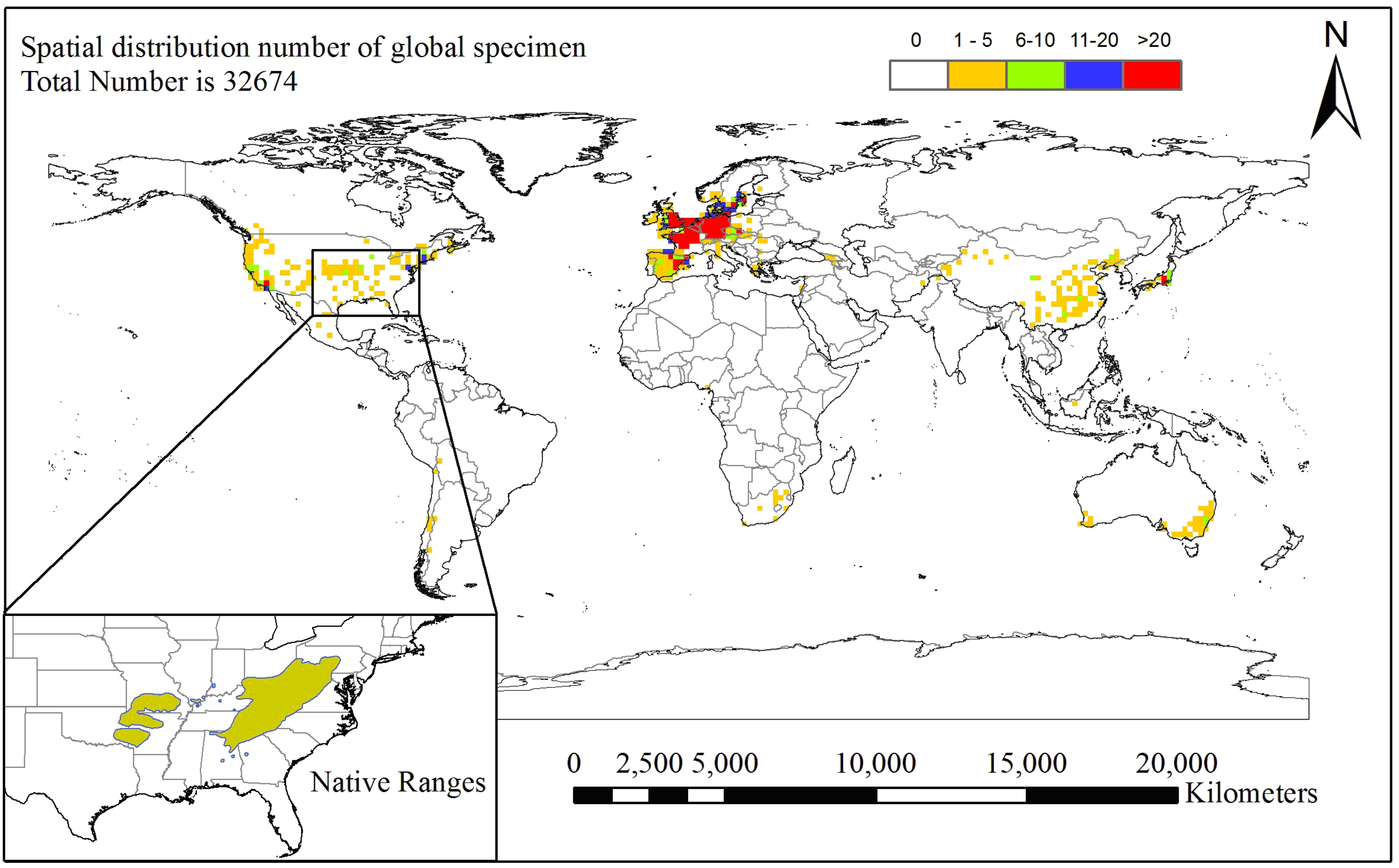
2.1. Species Occurrence Data
2.2. Climatic Variables

| Variable | Abbreviation | Unit | Formula and Reference |
|---|---|---|---|
| Annual mean temperature | AMT | °C | - |
| Mean temperature of the warmest month | MTWM | °C | - |
| Mean temperature of the coldest month | MTCM | °C | - |
| Annual range of temperature | ART | °C | Max temperature of warmest month-Min temperature of coldest month |
| Annual precipitation | AP | mm | - |
| Precipitation of wettest month | PWM | mm | - |
| Precipitation of driest month | PDM | mm | - |
| Precipitation of seasonality | PSD | - | Monthly coefficient of variation |
| Annual biotemperature | ABT | °C | ABT = (∑T)/12 (T is 0 < T < 30 °C mean month temperature) [30] |
| Warmth index | WI | °C | WI = ∑(T-5) (T is >5 °C mean month temperature) [38] |
| Coldness index | CI | °C | CI = ∑(T-5) (T is <5 °C mean month temperature) [42] |
| Potential evapotranspiration | PET | mm | PER = 58.93 × ABT/AP (ABT is annual biotemperature, AP is annual precipitation) [30] |
| Humidity index | HI | mm/°C | HI = AP/WI (AP is annual precipitation, WI is the warmth index) [46] |
2.3. Model Selection and Evaluation
2.4. Experimental Design and Statistical Analysis
3. Results
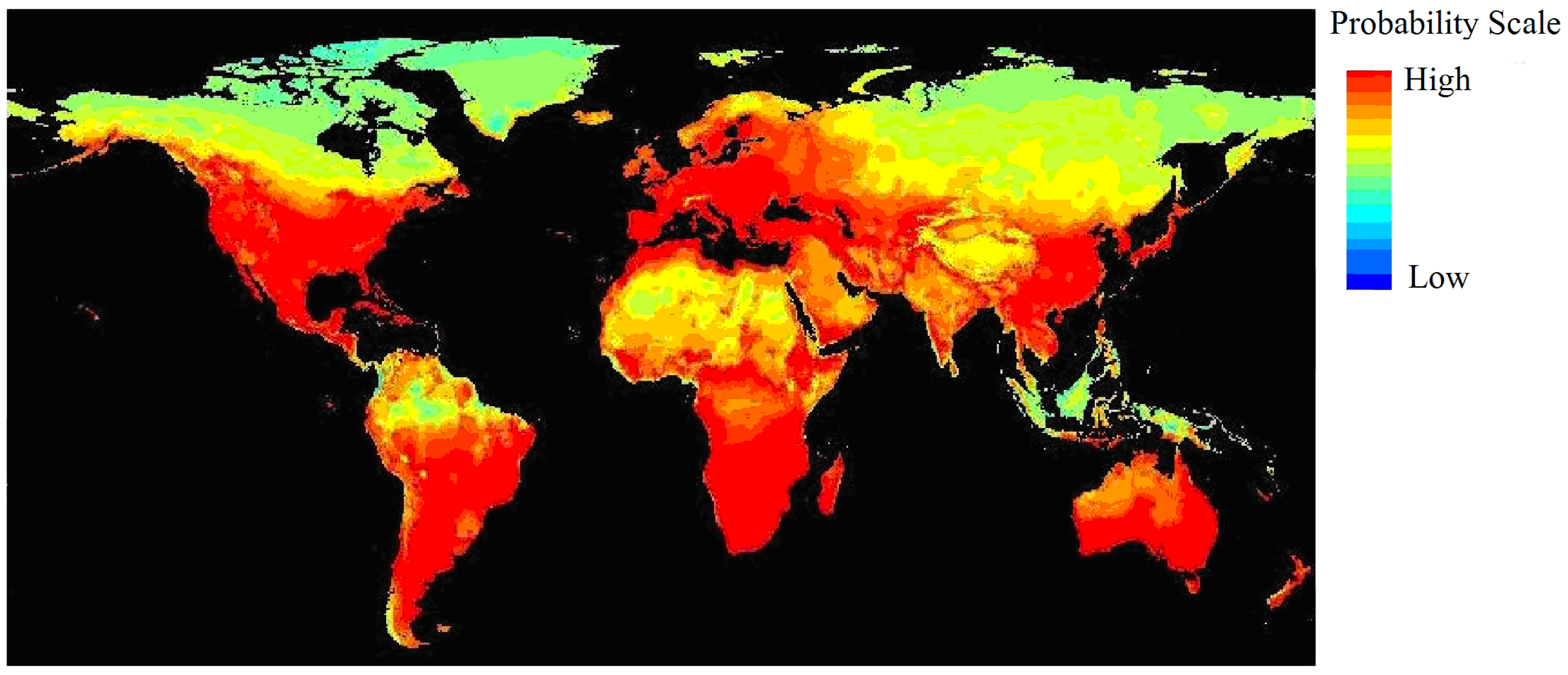
3.1. Current and Potential Distribution of Black Locust
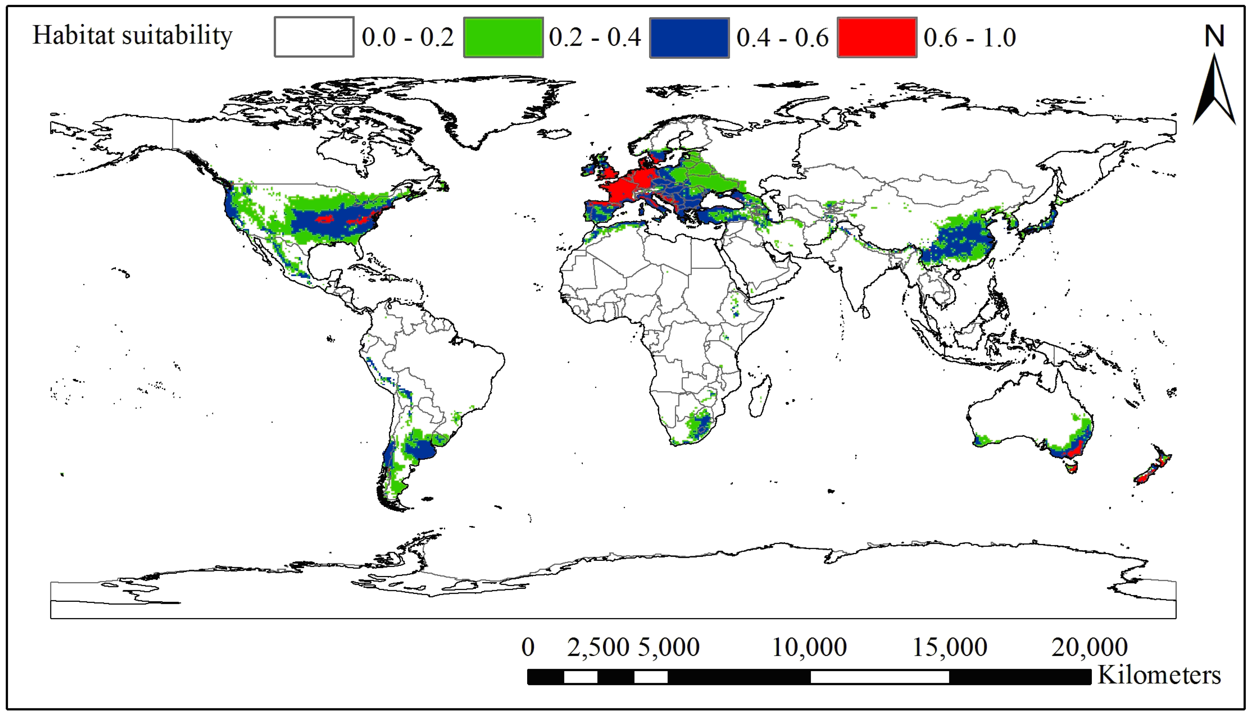
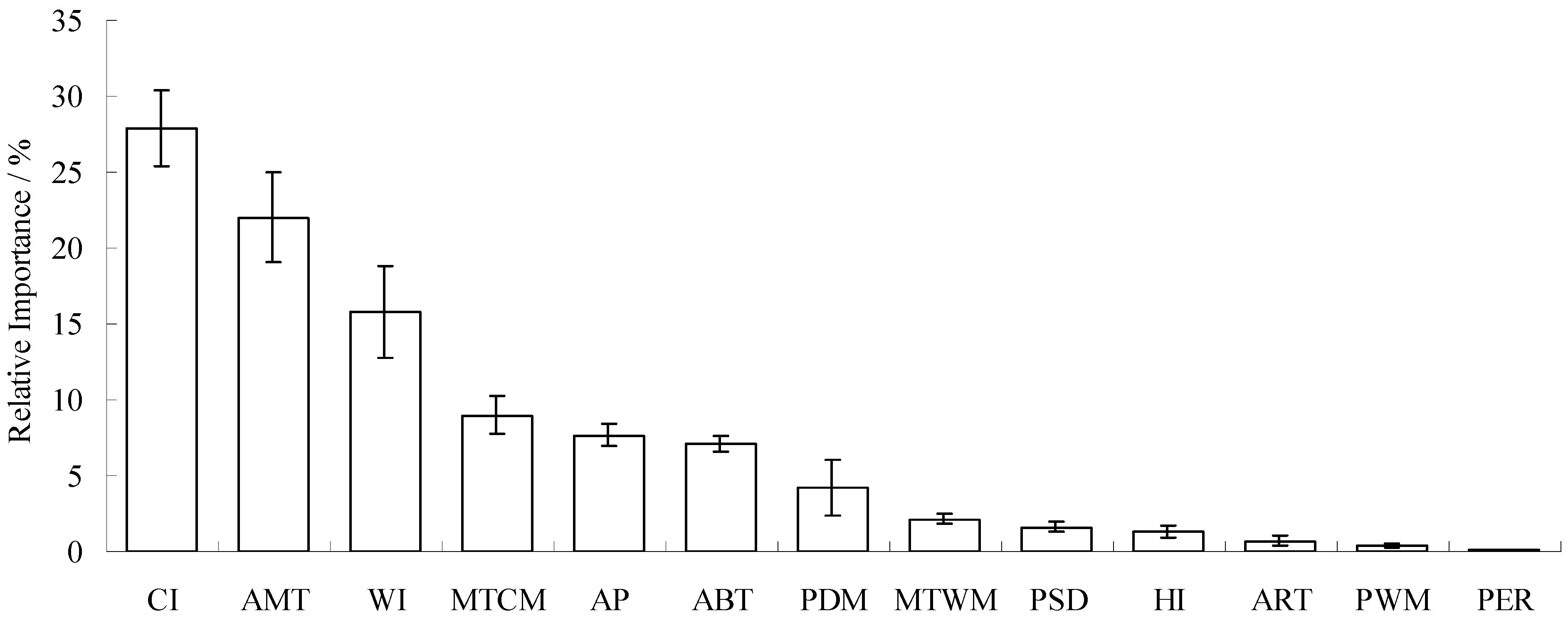
| Climatic Factor | Relative Importance % | Climatic Suitable Habitat Map | |||
|---|---|---|---|---|---|
| Core Area 0.6–1.0 | Moderately Suitable Area 0.4–0.6 | Marginal Area 0.2–0.4 | Unsuitable Area 0–0.2 | ||
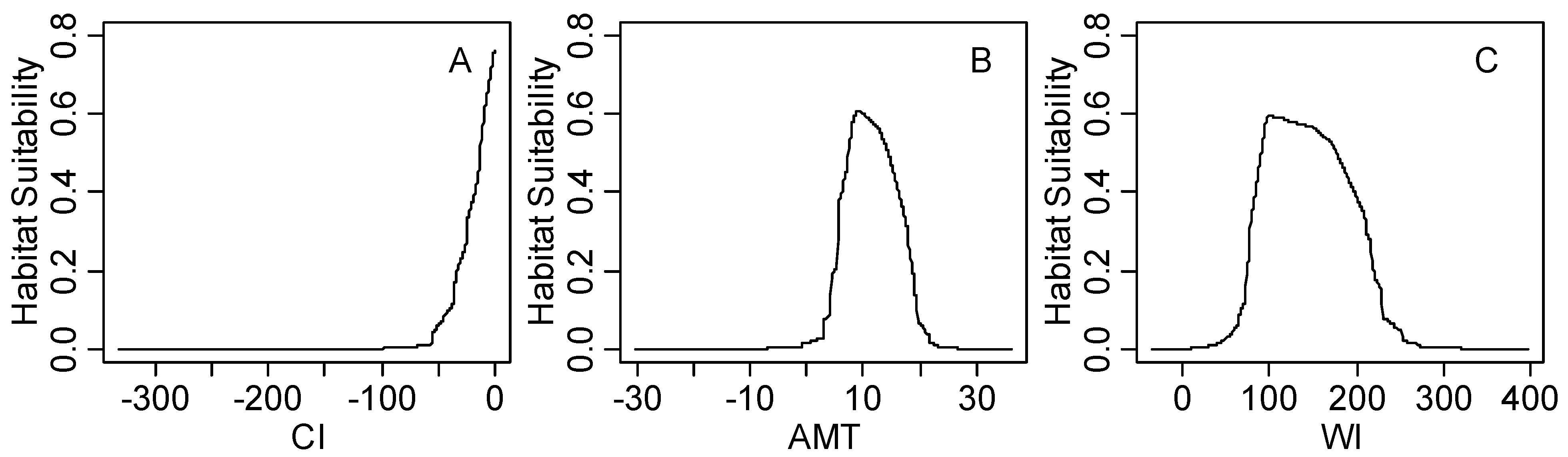
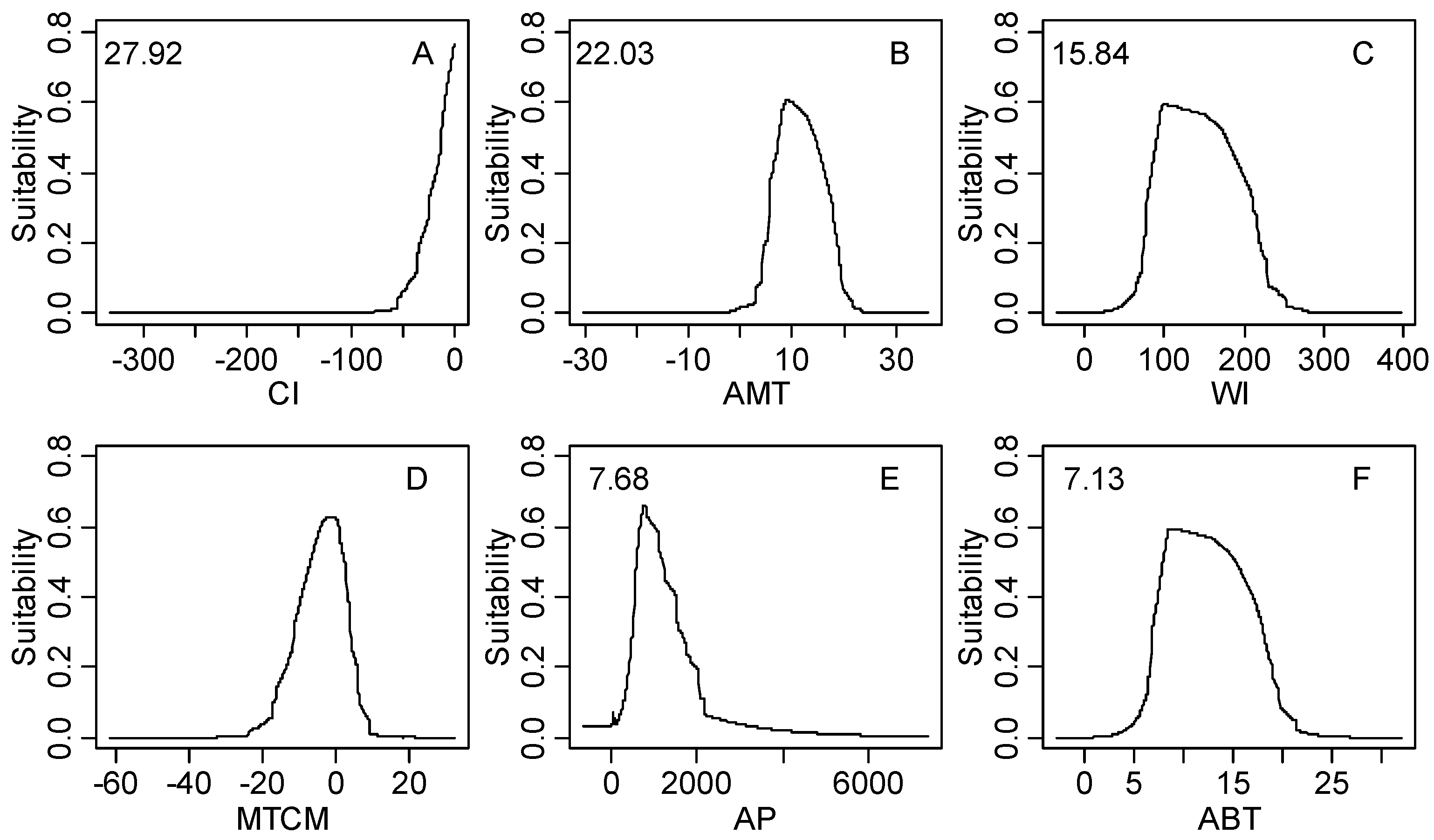
| CI | 27.92 | −9.8–0.0 | −26.0–0.0 | −59.7–0.0 | −328.2–0.0 |
| AMT | 22.03 | 5.8–14.5 | 3.9–18.4 | −1.8–22.0 | −26.9–31.3 |
| WI | 15.84 | 66.0–168.0 | 48.7–215.5 | 14.1–258.1 | 0.0–369.9 |
| MTCM | 8.96 | −9.5–5.5 | −15.3–6.3 | −22.1–13.0 | −54.7–25.6 |
| AP | 7.68 | 508.0–1867.0 | 298.0–3199.0 | 34.0–3309.0 | 0.0–8088.0 |
| ABT | 7.13 | 5.9–14.5 | 4.4–18.4 | 1.4–22.0 | 0.0–29.4 |
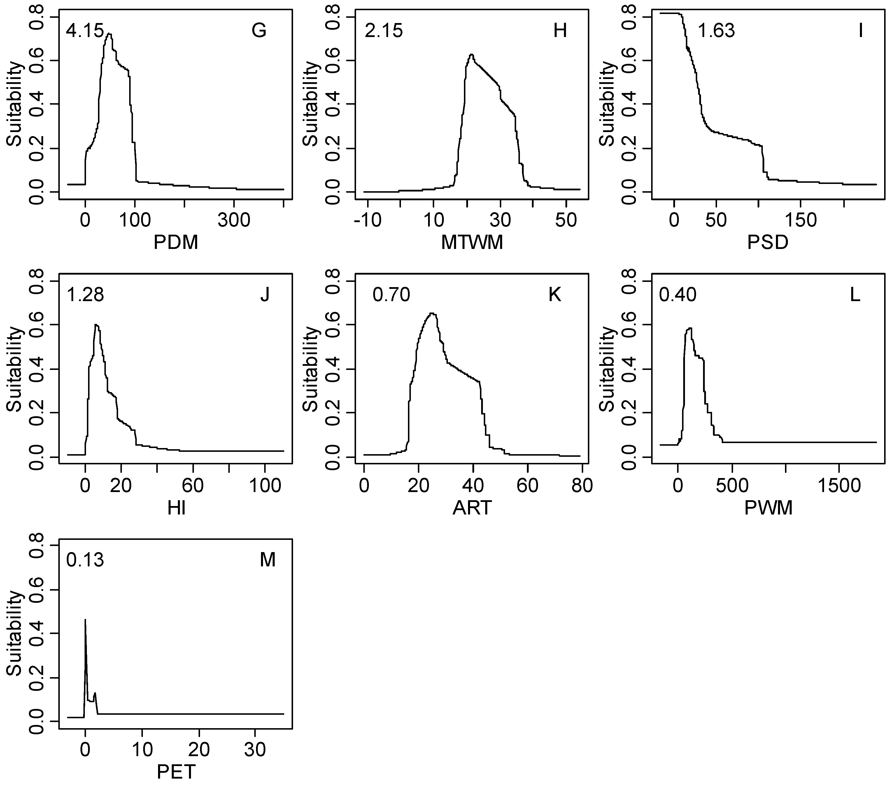
| PDM | 4.15 | 3.0–93.0 | 1.0–99.0 | 0.0–187.0 | 0.0–492.0 |
| MTWM | 2.15 | 18.0–33.2 | 17.1–39.1 | 11.9–39.4 | −5.9–48.8 |
| PSD | 1.63 | 7.0–101.0 | 6.0–143.0 | 7.0–140.0 | 0.0–261.0 |
| HI | 1.28 | 4.7–19.1 | 2.1–31.2 | 0.2–49.8 | 0.0–100.0 |
| ART | 0.70 | 16.3–40.2 | 16.3–44.2 | 12.4–52.0 | 5.4–72.4 |
| PWM | 0.40 | 52.0–246.0 | 47.0–507.0 | 8.0–749.0 | 0.0–1728.0 |
| PET | 0.13 | 0.2–1.0 | 0.1–2.3 | 0.1–19.4 | 0.0–1508.6 |
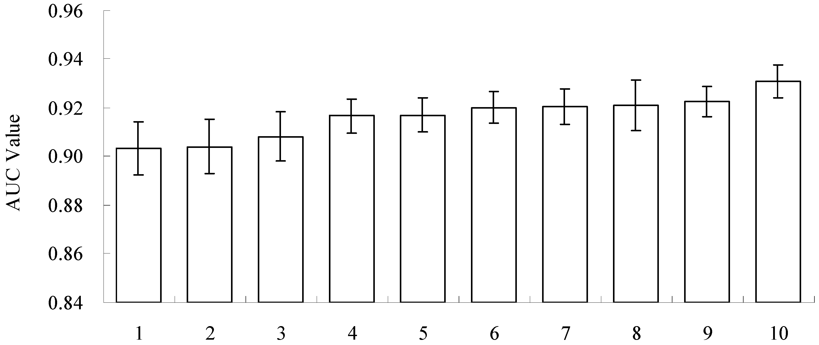
3.2. Model Performance and Importance of Climatic Factors

4. Discussion
4.1. Species Record Database and Species Modeling Tools
4.2. Significant Climatic Factors, Geographical Boundary and Potential Distribution Area
4.3. Climatic Threshold and Its Implication
5. Conclusions
Acknowledgments
Author Contributions
Supplementary


Conflicts of Interest
References
- Little, E.L. Atlas of United States trees. In Conifers and Important Hardwoods; US Department of Agriculture, Forest Service: Washington, DC, USA, 1971. [Google Scholar]
- Delectis Florae Reipublicae Popularis Sinicae Agendae Academiae Sinicae Edita. In Flora Reipublicae Popularis Sinicae; Science Press: Beijing, China, 1994; p. 228.
- Huntley, J.C. Robinia pseudoacacia L. Black locust. In Silvics of North America; Hardwoods, Agriculture Handbook, No. 654.; Burns, R.M., Honkala, B.H., Eds.; USDA Forest Service: Washington, DC, USA, 1990; pp. 755–761. [Google Scholar]
- Keresztesi, B. The black locust. Unasylva 1980, 32, 23–33. [Google Scholar]
- Cheeke, P.R. Black locust forage as an animal foodstuff. In Proceedings of the International Conference on Black Locust: Biology, Culture, & Utilization; Hanover, J.W., Miller, K., Plesko, S., Eds.; Department of Forestry, Michigan State University: East Lansing, MI, USA, 1992; pp. 252–258. [Google Scholar]
- Bridgen, M.R. Plantation silviculture of black locust. In Proceedings of the International Conference on Black Locust: Biology, Culture, & Utilization; Hanover, J.W., Miller, K., Plesko, S., Eds.; Department of Forestry, Michigan State University: East Lansing, MI, USA, 1992; pp. 21–32. [Google Scholar]
- Gupta, R.K. Multipurpose Trees for Agroforestry and Wasteland Utilisation; Oxford & IBH Publishing Co.: New Delhi, India, 1993. [Google Scholar]
- Haysom, K.A.; Murphy, S.T. The Status of Invasiveness of Forest Tree Species Outside Their Natural Habitat: A Global Review and Discussion Paper; Forest Health and Biosecurity Working Paper FBS/3E; FAO: Rome, Italy, 2003. [Google Scholar]
- Richardson, D.M.; Rejmanek, M. Trees and shrubs as invasive alien species—A global review. Divers. Distrib. 2011, 17, 788–809. [Google Scholar] [CrossRef]
- Randall, R.P. A Global Compendium of Weeds, 2nd ed.Department of Agriculture and Food: Perth, West Australia, Australia, 2012.
- Cierjacks, A.; Kowarik, I.; Joshi, J.; Hempel, S.; Ristow, M.; Vonderlippe, M.; Weber, E. Biological flora of the British Isles: Robinia pseudoacacia. J. Ecol. 2013, 101, 1623–1640. [Google Scholar] [CrossRef]
- Guisan, A.; Thuiller, W. Predicting species distribution: Offering more than simple habitat models. Ecol. Lett. 2005, 8, 993–1009. [Google Scholar] [CrossRef]
- Elith, J.; Graham, C.H.; Anderson, R.P.; Dudik, M.; Ferrier, S.; Guisan, A.; Hijmans, R.J.; Huettman, F.; Leathwick, J.R.; Lehmann, A.; et al. Nevel methods improve prediction of species’s distribution from occurrence data. Ecography 2006, 29, 129–151. [Google Scholar] [CrossRef]
- Franklin, J. Mapping Species Distributions: Spatial Interence and Prediction; Cambridge University Press: Cambridge, UK, 2009. [Google Scholar]
- Booth, T.H.; Nix, H.A.; Busby, J.R.; Hutchinson, M.F. BIOCLIM: The first species distribution modelling package, its early applications and relevance to most current MAXENT studies. Divers. Distrib. 2014, 20, 1–9. [Google Scholar] [CrossRef]
- Booth, T.H.; Nix, H.A.; Hutchinson, M.F.; Jovanovic, T. Niche analysis and tree species introduction. For. Ecol. Manag. 1988, 23, 47–59. [Google Scholar] [CrossRef]
- Hutchinson, G.E. Concluding remarks. Cold Spring Harb. Symp. Quant. Biol. 1957, 22, 415–427. [Google Scholar] [CrossRef]
- Peterson, A.T.; Soberon, J.; Pearson, R.G.; Andersen, R.P.; Martinez-Meyer, E.; Nakamura, M.; Araujo, M.B. Ecological Niches and Geographic Distributions; Monographsin Population Biology No. 49; Princeton University Press: Princeton, NJ, USA, 2011. [Google Scholar]
- Hijmans, R.J.; Cameron, S.E.; Parra, J.L.; Jones, P.G.; Jarvis, A. Very high resolution interpolated climate surfaces for global land areas. Int. J. Climat. 2005, 25, 1965–1978. [Google Scholar] [CrossRef]
- Jetz, W.; McPherson, J.M.; Guralnick, R.P. Integrating biodiversity distribution knowledge: Toward a global map of life. Trends Ecol. Evol. 2012, 27, 151–159. [Google Scholar] [CrossRef] [PubMed]
- Beck, J.; Ballesteros-Mejia, L.; Nagel, P.; Kitching, I.J. Online solutions and the “Wallacean shortfall”: What does GBIF contribute to our knowledge of species’ ranges? Divers. Distrib. 2013, 19, 1043–1050. [Google Scholar] [CrossRef]
- Booth, T.H. Using biodiversity databases to verify and improve descriptions of tree species climatic requirements. For. Ecol. Manag. 2014, 315, 95–102. [Google Scholar] [CrossRef]
- Tsoar, A.; Allouche, O.; Steinitz, O.; Rotem, D.; Kadmon, R. A comparative evaluation of presence-only methods for modeling species distribution. Divers. Distrib. 2007, 13, 397–405. [Google Scholar] [CrossRef]
- Wisz, M.S.; Hijmans, R.J.; Li, J.; Peterson, A.T.; Graham, C.H.; Guisan, A.; Group, N.P.S.D.W. Effects of sample size on the performance of species distribution models. Divers. Distrib. 2008, 14, 763–773. [Google Scholar] [CrossRef]
- Phillips, S.J.; Anderson, R.P.; Schapire, R.E. Maximum entropy modeling of species geographic distributions. Ecol. Model. 2006, 190, 231–259. [Google Scholar] [CrossRef]
- Phillips, S.J.; Dudik, M.; Elith, J.; Graham, C.H.; Lehmann, A.; Leathwick, J.; Ferrier, S. Sample selection bias and presence-only distribution models: Implications for background and pseudo-absence data. Ecol. Appl. 2009, 19, 181–197. [Google Scholar] [CrossRef] [PubMed]
- Slater, H.; Michael, E. Predicting the current and future potential distributions of Lymphatic filariasis in africa using maximum entropy ecological niche modelling. PLoS One 2012, 7, e32202. [Google Scholar] [CrossRef]
- Yin, X.J.; Zhou, G.S.; Sui, X.H.; He, Q.J.; Li, R.P. Dominant climatic factors of Quercus mongolica geographical distribution and their thresholds. Acta Ecol. Sin. 2013, 33, 103–109. [Google Scholar] [CrossRef]
- Merow, C.; Smith, M.J.; Silander, J.A. A practical guide to MaxEnt for modeling species’ distributions: What it does, and why inputs and settings matter. Ecography 2013, 36, 1058–1069. [Google Scholar] [CrossRef]
- Holdridge, L.R. Determination of world plant formations from simple climatic data. Science 1947, 105, 367–368. [Google Scholar] [CrossRef] [PubMed]
- Woodward, F.I. Climate and Plant Distribution; Cambridge University Press: Cambridge, UK, 1987. [Google Scholar]
- Pearson, R.G.; Dawson, T.P. Predicting the impacts of climate change on the distribution of species: Are bioclimate envelope models useful? Glob. Ecol. Biogeogr. 2003, 12, 361–371. [Google Scholar] [CrossRef]
- Guisan, A.; Tingley, R.; Baumgartner, J.B.; Naujokaitis-Lewis, I.; Sutcliffe, P.R.; Tulloch, A.I.T.; Regan, T.J.; Brotons, L.; McDonald-Madden, E.; Mantyka-Pringle, C.; et al. Predicting species distributions for conservation decisions. Ecol. Lett. 2013, 16, 1424–1435. [Google Scholar] [CrossRef]
- Global Biodiversity Information Facility. Available online: http://www.gbif.org/ (accessed on 9 May 2014).
- Chinese Virtual Herbarium. Available online: http://www.cvh.org.cn/ (accessed on 10 May 2014).
- Ballesteros-Mejia, L.; Kitching, I.J.; Jetz, W.; Nagel, P.; Beck, J. Mapping the biodiversity of tropical insects: Species richness and inventory completeness of African sphingid moths. Glob. Ecol. Biogeogr. 2013, 22, 586–595. [Google Scholar] [CrossRef]
- WorldClim—Global Climate Data. Available online: http://www.worldclim.org/ (accessed on 10 May 2014).
- Kira, T. A New Classification of Climate in Eastern Asia as the Basis for Agricultural Geography; Horticultural Institute, Kyoto University: Kyoto, Japan, 1945. [Google Scholar]
- Acosta, L.E. Distribution of Geraeocormobius sylvarum (Opiliones, Gonyleptidae): Range modeling based on bioclimatic variables. J. Arachnol. 2008, 36, 574–582. [Google Scholar] [CrossRef]
- Livshultz, T.; Mead, J.V.; Goyder, D.J.; Brannin, M. Climate niches of milkweeds with plesiomorphic traits (Secamonoideae; Apocynaceae) and the milkweed sister group link ancient African climates and floral evolution. Am. J. Bot. 2011, 98, 1966–1977. [Google Scholar] [CrossRef] [PubMed]
- Li, G.Q.; Liu, C.C.; Liu, Y.G.; Yang, J.; Zhang, X.S.; Guo, K. Effects of climate, disturbance and soil factors on the potential distribution of liaotung oak (Quercus wutaishanica Mayr) in China. Ecol. Res. 2012, 27, 427–436. [Google Scholar] [CrossRef]
- Kira, T. On the altitudinal arrangement of climatic zones in Japan. Kanchi-Nougaku 1948, 2, 143–173. [Google Scholar]
- Fang, J.Y.; Lechowicz, M.J. Climatic limits for the present distribution of beech (Fagus L.) species in the world. J. Biogeogr. 2006, 33, 1804–1819. [Google Scholar] [CrossRef]
- Ni, J.; Song, Y.C. Relationships between geographical distribution of Cyclobalanopsis glauca and climate in China. Acta Bot. Sin. 1997, 39, 451–460. [Google Scholar]
- Yim, Y.J. Distribution of forest vegetation and climate in the Korean Peninsula. III Distribution of tree species along the thermal gradient. Jpn. J. Ecol. 1977, 27, 269–278. [Google Scholar]
- Xu, W.D. Kira’s temperature indices and their application in the study of vegetation. Chin. J. Ecol. 1985, 3, 35–39. [Google Scholar]
- Maxent Software for Species Habitat Modeling. Available online: http://www.cs.princeton.edu/~schapire/maxent/ (accessed on 10 May 2014).
- Phillips, S.J.; Dudik, M.; Schapire, R.E. A maximum entropy approach to species distribution modeling. In Proceedings of the Twenty-First International Conference on Machine Learning, South Banff, Alberta, Canada, 4–8 July 2004; pp. 655–662.
- Stockwell, D.; Peters, D. The GARP modelling system: Problems and solutions to automated spatial prediction. Int. J. Geogr. Inf. Sci. 1999, 13, 143–158. [Google Scholar] [CrossRef]
- Yost, A.C.; Petersen, S.L.; Gregg, M.; Miller, R. Predictive modeling and mapping sage grouse (Centrocercus urophasianus) nesting habitat using Maximum Entropy and a long-term dataset from Southern Oregon. Ecol. Inform. 2008, 3, 375–386. [Google Scholar] [CrossRef]
- Baldwin, R.A. Use of maximum entropy modeling in wildlife research. Entropy 2009, 11, 854–866. [Google Scholar] [CrossRef]
- Fielding, A.H.; Bell, J.F. A review of methods for the assessment of prediction errors in conservation presence/absence models. Envir. Conser. 1997, 24, 38–49. [Google Scholar] [CrossRef]
- Swets, J. Measuring the accuracy of diagnostic systems. Science 1988, 240, 1285–1293. [Google Scholar] [CrossRef] [PubMed]
- Old Interface of GBIF. Available online: http://data.gbif.org/ (accessed on 10 May 2014).
- Prentice, I.C.; Cramer, W.; Harrison, S.P.; Leemans, R.; Monserud, R.A.; Solomon, A.M. A global biome model based on plant physiology and dominance, soil properties and climate. J. Biogeogr. 1992, 19, 117–134. [Google Scholar] [CrossRef]
- Peng, C.H. From static biogeographical model to dynamic global vegetation model: A global perspective on modelling vegetation dynamics. Ecol. Model. 2000, 135, 33–54. [Google Scholar] [CrossRef]
- Hong, B.G.; Li, S.Z. The preliminary study of the correlations between the distribution of main everygreen broad-leaf tree species in Jiangsu and climates. Acta Ecol. Sin. 1981, 1, 101–111. [Google Scholar]
- Irfan-Ullah, M.; Amarnath, G.; Murthy, M.S.R.; Peterson, A.T. Mapping the geographic distribution of Aglaia bourdillonii gamble (Meliaceae), an endemic and threatened plant, using ecological niche modeling. Biodivers. Conserv. 2007, 16, 1917–1925. [Google Scholar] [CrossRef]
- Chuine, I. Why does phenology drive species distribution? Philos. Trans. R. Soc. B 2010, 365, 3149–3160. [Google Scholar] [CrossRef]
- Petitpierre, B.; Kueffer, C.; Broennimann, O.; Randin, C.; Daehler, C.; Guisan, A. Climatic niche shifts are rare among terrestrial plant invaders. Science 2012, 335, 1344–1348. [Google Scholar] [CrossRef] [PubMed]
- Wang, M.C.; Wang, J.X.; Shi, Q.H.; Zhang, J.S. Photosynthesis and water use efficiency of platycladus orientalis and Robinia pseudoacacia saplings under steady soil water stress during different stages of their annual growth period. J. Integr. Plant Biol. 2007, 49, 1470–1477. [Google Scholar] [CrossRef]
© 2014 by the authors; licensee MDPI, Basel, Switzerland. This article is an open access article distributed under the terms and conditions of the Creative Commons Attribution license (http://creativecommons.org/licenses/by/4.0/).
Share and Cite
Li, G.; Xu, G.; Guo, K.; Du, S. Mapping the Global Potential Geographical Distribution of Black Locust (Robinia Pseudoacacia L.) Using Herbarium Data and a Maximum Entropy Model. Forests 2014, 5, 2773-2792. https://doi.org/10.3390/f5112773
Li G, Xu G, Guo K, Du S. Mapping the Global Potential Geographical Distribution of Black Locust (Robinia Pseudoacacia L.) Using Herbarium Data and a Maximum Entropy Model. Forests. 2014; 5(11):2773-2792. https://doi.org/10.3390/f5112773
Chicago/Turabian StyleLi, Guoqing, Guanghua Xu, Ke Guo, and Sheng Du. 2014. "Mapping the Global Potential Geographical Distribution of Black Locust (Robinia Pseudoacacia L.) Using Herbarium Data and a Maximum Entropy Model" Forests 5, no. 11: 2773-2792. https://doi.org/10.3390/f5112773
APA StyleLi, G., Xu, G., Guo, K., & Du, S. (2014). Mapping the Global Potential Geographical Distribution of Black Locust (Robinia Pseudoacacia L.) Using Herbarium Data and a Maximum Entropy Model. Forests, 5(11), 2773-2792. https://doi.org/10.3390/f5112773