Boosting Tree Stem Sectional Volume Predictions Through Machine Learning-Based Stem Profile Modeling

Abstract

Knowledge of the reduction in tree stem diameter with increasing height is considered significant for reliable tree taper prediction. Tree taper modeling offers a comprehensive framework that connects tree form to growth processes, enabling precise estimates of volume and biomass. In this context, machine learning modeling approaches offer strong potential for predicting difficult-to-measure field biometric variables, such as tree stem diameters. Two promising machine learning approaches, temporal convolutional networks (TCNs) and extreme gradient boosting (XGBoost), were evaluated for their ability to accurately predict trees’ stem profiles, suggesting a powerful and safe strategy for predicting tree stem sectional volume with minimal ground-truth measurements. The comparative analysis of TCN- and XGBoost-constructed models showed their strong ability to capture the taper trend of the trees. XGBoost proved particularly well adapted to the stem profile of black pine (Pinus nigra) trees in the Karya forest of Mount Olympus, Greece, by summarizing its spatial structure, substantially improving the accuracy of total stem volume up to RMSE% equal to 3.71% and 7.94% of all ranges of the observed stem volume for the fitting and test data sets. The same trend was followed for the 1 m sectional mean stem-volume predictions. The tested machine learning methodologies provide a stable basis for robust tree stem volume predictions, utilizing easily obtained field measurements.

1. Introduction

Considering the need for sustainable forest management, total tree stem volume can serve as the quantitative basis for determining the timber that can be safely harvested from the forest, as it provides the required accurate information for stand-level growing stock estimation and prediction. Reliable total stem volume estimation and prediction are not only crucial criteria for harvesting. Through this information, the growth and yield of forest stands can be accurately predicted, enabling the assessment of carbon stocks and informed long-term forest management planning [1].

Knowledge of tree stem sectional volume is fundamental in forestry, as it supports forest stand management strategies along with informed decision-making for wood utilization in the forest-based industry. Accurate estimation and prediction of sectional stem volumes require detailed information on the stem profile. Standard sectional volume equations widely used in forestry, such as Huber’s and Smalian’s formulas [2,3], which are based on multiple diameter measurements taken at closely spaced heights along the stem, require time and resources. Consequently, a more efficient and commonly adopted approach for describing diameter variation with height—namely, modeling the stem profile—is the use of taper functions, which are widely accepted in forestry research and practice [4,5].

Standard regression analysis is the most frequently used method for developing taper functions. Since Demaerschalk introduced polynomial taper equations in 1972 [6], and Max and Burkhart proposed segmented polynomial taper equations in 1976 [7], extensive research has been conducted in this field. For instance, flexible and widely adopted global variable-exponent taper equations were developed [8,9], and mixed-effects approaches were applied to account for tree- and stand-level variability during model development [10,11,12]. Although these approaches have been widely used, regression model development faces several challenges beyond the need to predefine a functional form. In particular, key statistical assumptions—such as independence, homoscedasticity, and normality of residuals—must be satisfied [13], which is often difficult with ground-truth forestry data. Violations of these assumptions can result in unstable models with reduced accuracy. While mixed-effects models are designed to address data correlation and heteroscedasticity [14], they still require the modeler to specify an appropriate functional form, and their generalization ability depends on the availability of calibration data [14,15].

Recently, substantial attention has been given to machine learning modeling approaches and algorithms. Owing to their nonparametric nature, these methods can address limitations associated with traditional regression analysis and have therefore been widely applied to modeling forest attributes at both stand and tree levels [16,17,18,19]. In taper modeling, Nunes et al. [20] recommended artificial neural networks for predicting taper and volume in complex tropical forest vegetation mosaics, outperforming six taper models from the literature. Similarly, Özçelik et al. [21] compared fixed-effects, mixed-effects, three- and five-quantile regression, and Levenberg–Marquardt artificial neural network approaches for estimating diameters along the boles of Scots pine (Pinus sylvestris) trees, finding that neural networks produced the most reliable results. Consistent with these findings, Sandoval and Acuña [22] reported that artificial neural networks outperformed conventional taper functions in a study on Nothofagus trees. Subsequently, Ko et al. [23] compared Kozak’s variable-exponent taper equation with several machine learning approaches for estimating stem profiles of Mongolian Oak (Quercus mongolica) trees and concluded that neural networks performed best. During the same period, Sağlam [24] compared segmented and variable-exponent taper models with random forest and XGBoost approaches and found that XGBoost effectively estimated stem profiles of Turkish pine (Pinus brutia) trees. Additionally, Diamantopoulou et al. [25] evaluated random forest as an alternative to ecoregional regression-based taper modeling and concluded that it produced highly reliable models with robust prediction intervals, as confirmed by uncertainty assessments. However, they also provided an extensive discussion of the algorithm’s limitations, which should be carefully considered during the modeling process [25].

Diameter measurements collected along a tree stem form the basis for characterizing stem profiles. Accurate estimation of these diameters enables calculation of sectional stem volume using standard, well-established forestry formulas such as Smalian’s formula [2,26]. However, because diameters are measured sequentially at increasing heights, the resulting data exhibit structural autocorrelation along the stem, which can complicate regression-based analyses [27].

To address this limitation, machine learning approaches that do not rely on distributional assumptions or predefined functional forms have been developed. These include sequential modeling algorithms such as recurrent neural networks (RNNs), temporal convolutional networks (TCNs), and related architectures. Several forestry studies have explored these methods. For example, Cywicka et al. [28] applied RNNs to model bark thickness profiles along stems and showed their superiority over traditional taper-curve methods, while Luković et al. [29] successfully used recurrent networks to fill gaps in high-frequency stem radius time series. More recently, Amir and Butt [30] applied four advanced RNN models to predict plant sap flow from stem diameter data, demonstrating improved predictive efficiency.

Although recurrent neural networks have received considerable attention, TCNs are relatively new yet powerful tools for sequential data modeling and remain underutilized in forestry research. For example, Pelletier et al. [31] applied TCNs to satellite image time-series classification and found that they outperformed random forests and RNNs commonly used in forest and land-cover mapping. Similarly, Kantavichai and Turnblom [32] demonstrated that TCN-based analysis of resistograph profiles can identify non-thrive trees for wood density prediction, and Duan et al. [33] confirmed the utility of TCNs for fine-scale forest classification. However, to date, no studies have investigated the application of TCNs to stem taper modeling. In parallel, the XGBoost modeling approach has recently been adopted in forest modeling because of its ability to capture nonlinear relationships and feature interactions [23,34,35]. Although XGBoost is not explicitly designed for sequential data, unlike TCNs, it is a robust gradient-boosted tree ensemble method that can reveal temporal patterns and growth rates, offer interpretability, and provide valuable insights for forestry management and ecological research [23,36,37].

This study had four main objectives: (a) to explore the nature of the primary stem diameters data of black pine (Pinus nigra) trees in the Karya forest; (b) to evaluate the capacity of two distinct machine learning modeling techniques, the TCN and the tree-based ensemble methodology XGBoost, to accurately represent the stem profile of Pinus nigra trees in the Karya forest of Mount Olympus, Greece; (c) to conduct a comparison between the two approaches, taking into account the accuracy of the trees’ stem sectional volume predictions that can be derived from the two machine learning modeling techniques; and finally (d) to suggest a powerful yet safe strategy for accurately predicting tree stem sectional volume, utilizing minimal ground-truth measurements.

2. Materials and Methods

2.1. Study Area and Ground-Truth Data

As the mythological home of the Greek gods, Mount Olympus, with a peak at 2917.73 m, is the highest mountain in Greece [38]. The region has a Mediterranean climate, characterized by dry summers and wet winters. The Olympus National Park is one of the most floristically rich areas of Greece, hosting approximately 1700 species and subspecies, about 25% of the country’s flora, within the evergreen broadleaf forest zone. Black pine (Pinus nigra) trees are included in the evergreen broadleaf zone of the Mount.

The Karya Forest on Mount Olympus is situated at an elevation of approximately 1400 m and covers an area of 103.64 hectares [39]. This forest (Figure 1) represents the region’s vegetation. It is worth noticing that hybrid fir (Abies borisii-regis) often forms mixed stands with Pinus nigra trees in this area. In recent decades, under the management practices applied by the Forest Service [39], which manages this area, hybrid fir has been favored. This has resulted in the remaining Pinus nigra trees being older and more sparsely distributed in the upper canopy [40]. In this direction, adaptive random sampling [41], as the best alternative option to conventional designs when the sampled characteristics are rare and spatially clustered [42], was used. Aiming to reduce over-representation and correlation, the representative coverage of both individual trees and clusters of Pinus nigra trees was assessed by measuring clusters at a reasonable distance from each other, relative to the height of the dominant tree, with spacing between clusters at least 1.5 times the dominant height of the cluster [40].

The measurements taken from the sample of standing tree stems included the stump (d_0.3) and breast height diameters (d_1.3), measured at 0.3 and 1.3 m above ground, respectively. Additionally, diameters at one-meter intervals from breast height to the top of each tree were measured using the Spiegel Relaskope (Spiegel Relaskop^®). The total stem height (tht) was measured with a Forestry Pro laser hypsometer (Nikon Forestry Pro II, Nikon Vision Co., Ltd., Tokyo, Japan), while the geographic position of each sampled tree was determined using a GPS device (Garmin eTrex 32xTopo Active Europe, Garmin International/Garmin Corporation, Kansas, MO, USA). To avoid errors caused by anomalies often found in the lower part of the tree stem, two perpendicular over-bark diameter measurements were taken at 0.3 and 1.3 m from the ground on the stem. The final values of d_0.3 and d_1.3 diameters were the average of two perpendicular measurements at each height. The final sample size used in the analysis included 4601 diameter measurements on two hundred twenty-one trees, with several subsequent diameter measurements on each tree, depending on each tree’s height.

2.2. Data Exploration

Initially, exploratory data analysis (EDA) [43] was used to understand the primary data configuration by identifying possible patterns, relationships, missing data, and extreme values. A very small percentage of missing values was detected, mainly due to poor visibility of the stem beneath the crown. The process of filling these gaps was achieved using the cascade correlation artificial neural network (CCANN) retrieval methodology described by [44]. Extreme values were not detected in the sample, and only a small percentage of values identified as outliers were retained to ensure that the population’s maximum variability was represented.

Diameter measurements taken at different heights on the same tree stem (e.g., diameter at height 0.3 m, 1.3 m, 2.3 m, etc.) are likely autocorrelated because of their spatial order. To identify potential spatial autocorrelation, the autocorrelation function (ACF) [45], based on the Wold representation theorem [46], was selected as a possible option. Since stationarity is a key assumption in ACF analysis, the second-order (weak) stationarity of tree stem diameter values was explored, as the tapering of the stem makes strict stationarity unreasonable. For this reason, and to create a complete picture of possible stationarity, diagnostics such as mean and variance profile plots, along with the augmented Dickey–Fuller (ADF) [47] and the Kwiatkowski–Phillips–Schmidt–Shin (KPSS) [48] statistical tests, were performed, respectively. The mean (Figure 2a) profile plot was produced by averaging the diameter at each height across all trees, while the variance (Figure 2b) profile plot showed the diameter variance at each height. Both figures (Figure 2) clearly showed a significant change in the mean and variance across heights, indicating non-stationarity.

In the same direction, for both the ADF and KPSS tests applied to each tree separately, the null hypothesis of stationarity was rejected in 86% of the trees, while in the remaining 14% the tests showed borderline or a trend of stationarity (significance level α = 0.05).

Given the non-stationary nature of diameters along the stem, as indicated by the diagnostics above, the detrended diameter profiles were fit with splines (Figure 3) for each tree to obtain stationary residuals, thereby isolating and removing local fluctuations from the overall tapering pattern.

The smoothing splines minimized the objective function:

$$\sum {\left[\left(d_i\right)-\sum \left(c_j·B_j\left(h_i\right)\right)\right]}^2+s·\int {\left[f^{″}\left(h\right)\right]}^{2}dh,$$

(1)

where $d_i$ is the observed diameter at height h_i, $B_j\left(h_i\right)$ is the B-spline basis function, c_j are the spline coefficients, s is the smoothing factor used, and $f″\left(h\right)$ is the second derivative of the spline function [$\sum \left(c_j·B_j\left(h_i\right)\right)$], which penalizes curvature.

Indicatively, the fit of different smoothing splines related to four different tree diameter profiles is shown in Figure 3. The cubic smoothing splines of Figure 3 represented the main taper trend of the trees. In contrast, the derived residuals represented deviations from the general trend due to the biological nature of tree growth.

ACF was applied to the detrended residuals for analyzing the diameter structure along the stem. This approach was considered essential for understanding trends in diameter growth, thereby improving the interpretability of the modeling approach to be used for reliable diameter prediction along the stem.

Finally, the total tree stem volume was calculated using the widely recognized Smalian’s segmented formula [2,3,26], applied to each 1 m stem segment. This formula uses the cross-sectional areas at the two ends of a segment, without requiring a midpoint area specification, along with the segment length, enabling minor errors per section, log scaling practices, and sectional volume tables, which can be very useful in forestry operations. However, Smalian’s formula tends to overestimate the volume of a neiloid log [49]. Considering its accepted accuracy by the forest community with the lowest formula complexity and the fact that Pinus nigra trees do not show a strong concave taper near the base as buttressed trees and those with root flare [50], Smalian’s formula was selected for the segmented stem volumes calculation.

2.3. Data Handling

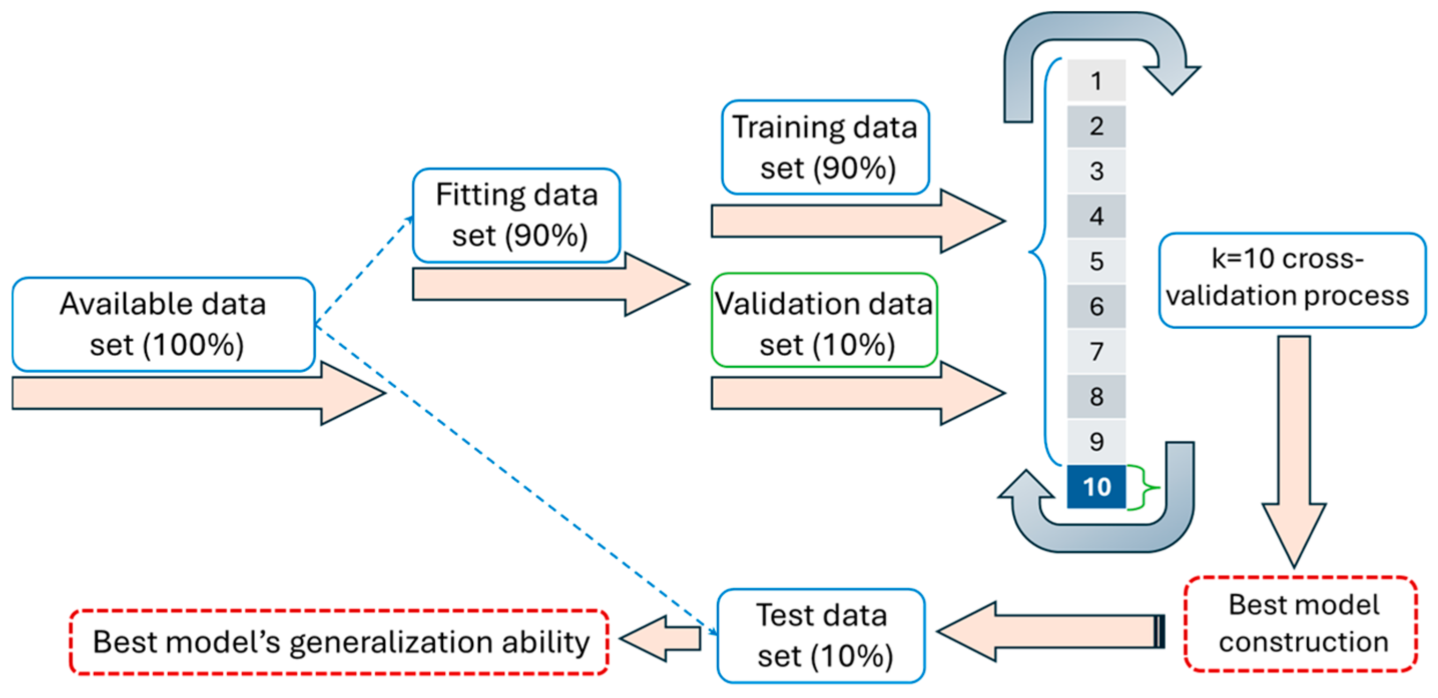
To proceed with model construction, the available dataset was randomly divided into a fitting set (approximately 90% of the total, comprising 4141 diameter measurements) and a test set (the remaining 10%, consisting of 460 diameter measurements). Random numbers were used for this purpose, and the split was applied to the trees rather than to their stem diameters. In addition, the k-fold cross-validation methodology was applied to the fitting data set with k = 10. In this way, the data was split into three distinct data sets: the training data, used for model training; the validation data, used for model tuning and selection; and the test data set, used for final model evaluation [51]. The division of the fitting data set was performed using k = 10 cross-validation. The data usage flowchart for model fitting and evaluation is shown in Figure 4.

Following the above-described division of the available data set, the descriptive statistics of the fitting and the test data sets are given in

Table 1. Descriptive statistics of tree attributes for the training and test datasets, including: stump diameter (d_0.3, cm), diameter at breast height (d_1.3, cm), total tree height (tht, m), total stem volume (v_tot, m³), and segmented stem volumes by one-meter intervals from stump to tip.

Variable	Mean	Std. Error of the Mean	Std. Deviation	Variable	Mean	Std. Error of the Mean	Std. Deviation
Fitting data set
d0.3	50.8080	1.3307	18.8186	v12.3–13.3	0.0513	0.0032	0.0439
d1.3	45.0015	1.2401	17.5370	v13.3–14.3	0.0457	0.0029	0.0392
tht	20.5825	0.3599	5.0893	v14.3–15.3	0.0392	0.0026	0.0346
vtot	1.5769	0.0905	1.2794	v15.3–16.3	0.0338	0.0023	0.0302
v0.3–1.3	0.2068	0.0102	0.1445	v16.3–17.3	0.0286	0.0021	0.0265
v1.3–2.3	0.1707	0.0088	0.1241	v17.3–18.3	0.0237	0.0018	0.0232
v2.3–3.3	0.1495	0.0078	0.1102	v18.3–19.3	0.0199	0.0017	0.0202
v3.3–4.3	0.1333	0.0070	0.0993	v19.3–20.3	0.0166	0.0015	0.0173
v4.3–5.3	0.1194	0.0065	0.0914	v20.3–21.3	0.0125	0.0014	0.0146
v5.3–6.3	0.1095	0.0061	0.0847	v21.3–22.3	0.0092	0.0012	0.0122
v6.3–7.3	0.0992	0.0057	0.0790	v22.3–23.3	0.0062	0.0010	0.0096
v7.3–8.3	0.0912	0.0053	0.0736	v23.3–24.3	0.0040	0.0009	0.0075
v8.3–9.3	0.0826	0.0049	0.0681	v24.3–25.3	0.0028	0.0008	0.0056
v9.3–10.3	0.0740	0.0046	0.0631	v25.3–26.3	0.0016	0.0006	0.0034
v10.3–11.3	0.0662	0.0042	0.0579	v26.3–27.3	0.0013	0.0006	0.0021
v11.3–12.3	0.0587	0.0037	0.0501	v27.3–28.3	0.0003	0.0002	0.0005
Test data set
d0.3	47.1636	4.0679	19.0802	v10.3–11.3	0.0596	0.0116	0.0518
d1.3	41.4364	3.8596	18.1029	v11.3–12.3	0.0525	0.0103	0.0463
tht	19.8955	1.1662	5.4698	v12.3–13.3	0.0457	0.0093	0.0417
vtot	1.3725	0.2565	1.2033	v13.3–14.3	0.0400	0.0085	0.0379
v0.3–1.3	0.1807	0.0287	0.1348	v14.3–15.3	0.0343	0.0077	0.0344
v1.3–2.3	0.1505	0.0251	0.1177	v15.3–16.3	0.0286	0.0069	0.0307
v2.3–3.3	0.1327	0.0226	0.1060	v16.3–17.3	0.0233	0.0059	0.0265
v3.3–4.3	0.1162	0.0203	0.0950	v17.3–18.3	0.0193	0.0052	0.0226
v4.3–5.3	0.1029	0.0183	0.0861	v18.3–19.3	0.0167	0.0048	0.0191
v5.3–6.3	0.1017	0.0175	0.0782	v19.3–20.3	0.0121	0.0039	0.0150
v6.3–7.3	0.0920	0.0166	0.0741	v20.3–21.3	0.0094	0.0035	0.0120
v7.3–8.3	0.0842	0.0158	0.0707	v21.3–22.3	0.0091	0.0032	0.0090
v8.3–9.3	0.0759	0.0147	0.0657	v22.3–23.3	0.0059	0.0022	0.0058
v9.3–10.3	0.0670	0.0130	0.0583	v23.3–24.3	0.0030	0.0012	0.0033

. Table 1 includes the arithmetical mean, the standard error of the mean and the standard deviation of the observed d_0.3, and d_1.3, both in cm, the total tree height (tht) in m, the total stem volume (v_tot) calculated as the summation of the segmented stem volumes by one-meter intervals from stump to tip plus the volume of the top section with length < 1 m of the tree which considered as a cone section and the segmented stem volumes by one-meter intervals from stump to tip, all calculated by the Smalian’s formula in cubic meters.

The tree identification number, the height at location i on the standing tree stem (h_i), and the diameter measurement at height i (d_hi) served as input variables for model development. Total tree height field-measured data were utilized to verify the actual number of diameter measurements collected for each stem, but were not included as a separate input variable in the models’ construction. Instead, this information was indirectly incorporated through the count of measured diameters per stem.

2.4. Temporal Convolutional Network (TCN) Modeling

TCN is designed to handle sequential data. It is built using multiple layers (convolutional layers, where a kernel filter is applied) [52]. Lower layers can capture local patterns, while higher layers can capture global temporal dependencies.

Gradient descent with backpropagation is used during training to determine the optimal values of the weights. The main characteristic of the system is its causality, meaning that the model cannot see future values when predicting the current step, preventing data leakage, unlike Convolutional Neural Networks (CNNs). At the same time, it can use dilated convolutions, meaning it can use back-step data from far away from the current step if desired. 1D causal convolution, with kernel = l, at step s is

$$\widehat{d}(s)={\sum }_{i=1}^{l-1}\left[w_i{·d}_{\left(s-{df}_i\right)}\right],$$

(2)

where $\widehat{d}\left(s\right)$ denotes the predicted value at time step s, $w_i$ are the kernel weights, which are optimized during training via gradient descent using backpropagation, $d_{\left(s-{df}_i\right)}$ represent the corresponding input values over the preceding time step s, and df (equals to one for a 1D convolution) is the dilation factor, which represents the spacing between kernels.

The error between prediction and observed diameter values is computed using the partial derivatives of the mean square error (MSE) (loss function):

$${\displaystyle \frac{\partial \left(\frac{1}{n}·\sum _{i=1}^n{\left(d_i-\widehat{d_i}\right)}^2\right)}{\partial w_{j }}},$$

(3)

where $d_i$ is the observed value at step s, $\widehat{d_i}$ is the prediction at step s, $w_j$ are the kernel weights which are learned during training using the gradient descent algorithm with backpropagation, and n is the sample size. The weights were updated continuously over many passes over the data set (epochs) using the learning rate (l) hyperparameter of training until the model minimizes the loss function.

The most significant hyperparameters that affect the training of the TCN model are: (a) the number of filters per layer (num_filters) which controls the dimensionality and the capacity of the model to learn complex patters, (b) the kernel size (kernel) which defines the width of the convolutional filter, (c) the learning rate (l) which controls the optimal convergence of the training, (d) the batch_size (batch_size) which affects the training stability and speed, and (e) the number of full pass through the entire training dataset (epochs).

The activation function used in the intermediate stages was selected among the exploration of five options (ReLU, SELU, Tanh, Sigmoid and ELU), which are recognized as effective in machine learning model building [53]. The training of the TCN model was applied using Scikit-learn and Keras libraries, along with the Optuna optimization framework, including a type of hyperparameters grid-search strategy in the Python language (v3.13.11) [54,55].

2.5. Extreme Gradient Boosting (XGBoost) Modeling

The XGBoost scalable framework [56] sequentially trains multiple weak learners (decision trees) and optimizes the prediction function by minimizing a regularized loss function via a second-order Taylor approximation. Each decision tree predicts the residuals derived from the previous learners, and the final prediction is derived by the summation of all learners:

$$\widehat{d_i}=lr·f_1\left(d_i\right)+lr·f_2\left(d_i\right)+\dots +lr·f_T\left(d_i\right)$$

(4)

where $\widehat{d_i}$ is the final diameter prediction, $f_1\left(d_i\right)$ is the residual derived by the initial prediction from the learner (1), lr is the learning rate used, which controls each tree’s contribution to the final diameter prediction, and T is the total number of sequential trees used.

To prevent overfitting and complexity, the L2 regularization term on the weights, which penalizes the squared coefficients, has been used.

Finally, the critical hyperparameters that required for the successful training of the XGBoost model construction, include the number of boosting rounds (decision trees, n_dt), the learning rate (lr) which controls each tree’s contribution to the final prediction, the number of branches which determine the depth of each tree (d_max), a parameter regulating the splitting to child node (mcw) acting as an additional regularization parameter by preventing too specific leaves, the reg_lambda regularization term, which adds an L2 penalty on the leaf weights of the decision trees, and the gamma (γ), which controls the decision tree complexity along with its depth.

The tuning of the significant hyperparameters for XGBoost model training was implemented using Optuna [55], along with early stopping to achieve the best possible training efficiency. Under Optuna’s search strategy, Bayesian optimization (Tree-structured Parzen Estimator) [57,58] was used, which can be thought of as an efficient search that learns from past trials to select the following best parameter combinations.

2.6. Evaluation Metrics

The implementation of the evaluation metrics took place in two stages. First, both constructed models (TCN and XGBoost) were evaluated for their global accuracy and reliability in predicting diameters along the tree stem, so that their diameter predictions could be safely used for further segmented tree stem volume predictions using Smalian’s formula. Second, the global accuracy and reliability in predicting total stem volume were assessed, along with the same metrics per volume segment, to examine how estimation and prediction errors are distributed relative to the segmented stem volumes.

The evaluation metrics used were:

(a)

The root mean square error (RMSE):

$$RMSE=\sqrt{{\displaystyle \frac{{\sum }_{i=1}^{i=n}{\left(y_i-{\widehat{y}}_i\right)}^2}{n}}}$$

(5)

(b)

The percentage root mean square error (RMSE%), expressed as the percentage error of the observed values average:

$$RMSE\%={\displaystyle \frac{\sqrt{\frac{{\sum }_{i=1}^{i=n}{\left(y_i-{\widehat{y}}_i\right)}^2}{n}}}{\overline{y}}}·100$$

(6)

(c)

The correlation coefficient:

$$R={\displaystyle \frac{{\sum }_{i=1}^{i=n}\left[\left(y_i-{\widehat{y}}_i\right)·\left(y_i-\widehat{\overline{y}}\right)\right]}{\sqrt{{\sum }_{i=1}^{i=n}\left[{\left(y_i-\overline{y}\right)}^2\right]}·\sqrt{{\sum }_{i=1}^{i=n}\left[\left(y_i-\widehat{\overline{y}}\right)\right]}}}$$

(7)

(d)

The average absolute error (AAE):

$$AAE={\displaystyle \frac{\sum _{i=1}^{i=n}\left|y_i-{\widehat{y}}_i\right|}{n}}$$

(8)

(e)

Relative (i) estimation/prediction and (ii) residuals plots

where y_i is the observed (i) value of the output variable, ${\widehat{y}}_i$ is the i estimation/prediction value of the output variable, $\widehat{\overline{y}}$ is the average value of the estimated/predicted values, $\overline{y}$ is the average value of the observed values and n is the related sample size.

3. Results

3.1. Stem Diameter Modeling

3.1.1. Autocorrelation

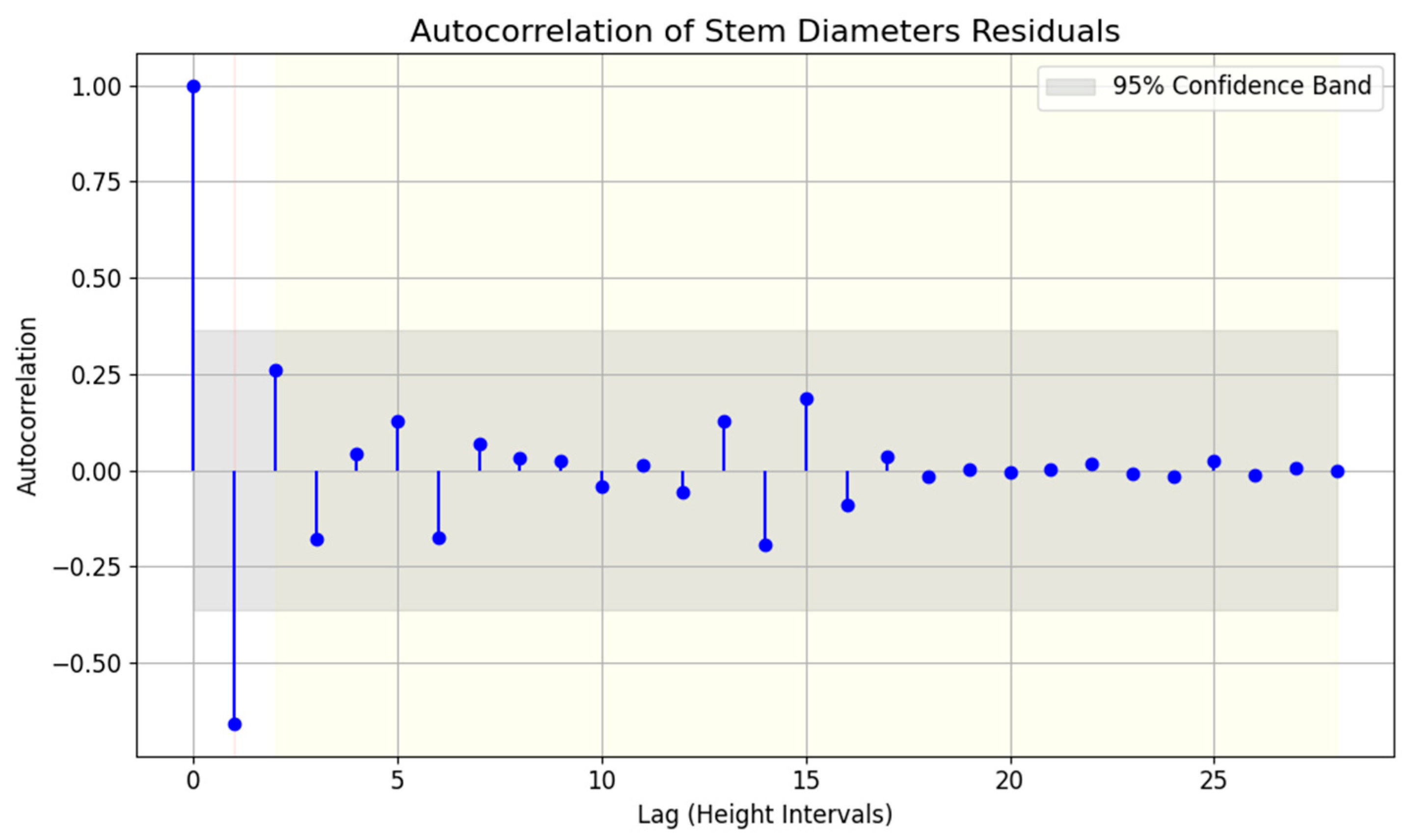
Following the results of the diameters’ spatial autocorrelation analysis of Section 2.2, which clearly showed the non-stationary nature of diameters along the tree stem, the ACF was applied to the detrended residuals for analyzing the diameter structure along the stem. Figure 5 shows the ACF plot for the overall pattern of fitting trees’ detrended residuals per height lag. Although the degree of autocorrelation waviness differed among individual trees, possibly reflecting differences in growth, branching, and biomechanical stress responses, Figure 5 clearly reflects the overall mean trend of all trees.

The most significant trend-related correlation was observed at lag 1, while the autocorrelation at the following lags was generally small within the 95% confidence band (Figure 5). For higher lags (above lag 17), the autocorrelation values were around zero (Figure 5). The overall values configuration reflected the way trees respond to mechanical stress and remain structurally stable. After removing the main taper trend (Figure 3), the autocorrelation configuration of the stem diameter residuals within each height interval showed that the stem diameter irregularities exhibited weak linear autocorrelation across height intervals, indicating short-range structured variation. However, autocorrelation functions, such as ACF, are limited to measuring linear, second-order relationships and do not capture nonlinear, higher-order, or context-dependent spatial patterns. Furthermore, individual trees exhibited distinct patterns of residuals, likely reflecting variations in growth history and branching. Therefore, the stem should be considered a spatially ordered biological structure in which local deviations are hierarchically integrated along the stem.

3.1.2. Machine Learning Modeling

The optimal hyperparameters tuning for both machine learning approaches was assessed using Optuna’s Bayesian optimization framework. The optimal combinations of all hyperparameters for the TCN and XGBoost models are shown in

Table 2. Optimal hyperparameter values combination for both the machine learning models.

Hyperparameters for the TCN Model
	num_filters	kernel	dilation_rate	learning_rate	batch_size	epochs
range	[64–128]	[1–5]	1	[0.001–0.1]	[16–64]	[30–100]
step	8	1	1	0.0001	8	5
optimal value	128	2	1	0.0036	16	80
Hyperparameters for the XGBoost Model
	ndt	lr	dmax	mcw	reg_lambda	γ
range	[100–200]	[0.10–0.30]	[1–6]	[0–2]	[0–5]	[0–5]
step	5	0.01	1	1	0.01	0.01
optimal value	185	0.28	5	1	1.44	0.11

.

Each hyperparameter for both modeling approaches was evaluated across predefined value ranges with specified steps. Furthermore, for the TCN model, ReLU was selected as the activation function based on its superior performance.

The evaluation metrics for the machine learning models in Table 2, both on the fitting and test data sets, are presented in

Table 3. Evaluation metrics for the machine learning modeling approaches, for the fitting and the test data sets.

Fitting Data Set
models	RMSE, cm	RMSE%	R	AAE, cm
TCN	1.2650	5.0930	0.9968	0.8819
XGBoost	1.0371	4.1757	0.9978	0.7526
Test Data Set
TCN	1.8672	7.9404	0.9936	1.2681
XGBoost	1.4836	6.3091	0.9952	1.0204

. The mean errors ranged from 1.265 to 1.0371 for the fitting data set, corresponding to 5.09% to 4.18% of the mean stem diameter values for both the TCN and XGBoost models, which are quite small and acceptable for both modeling approaches (Table 3).

In the same direction, the mean errors derived from both the constructed models ranged from 1.87 to 1.48 for the test data set unseen by the models, indicating higher errors of 2.01% and 2.13% of the mean stem diameter values for the TCN and XGBoost models, respectively (Table 3). These results indicate that both models demonstrate acceptable generalization performance.

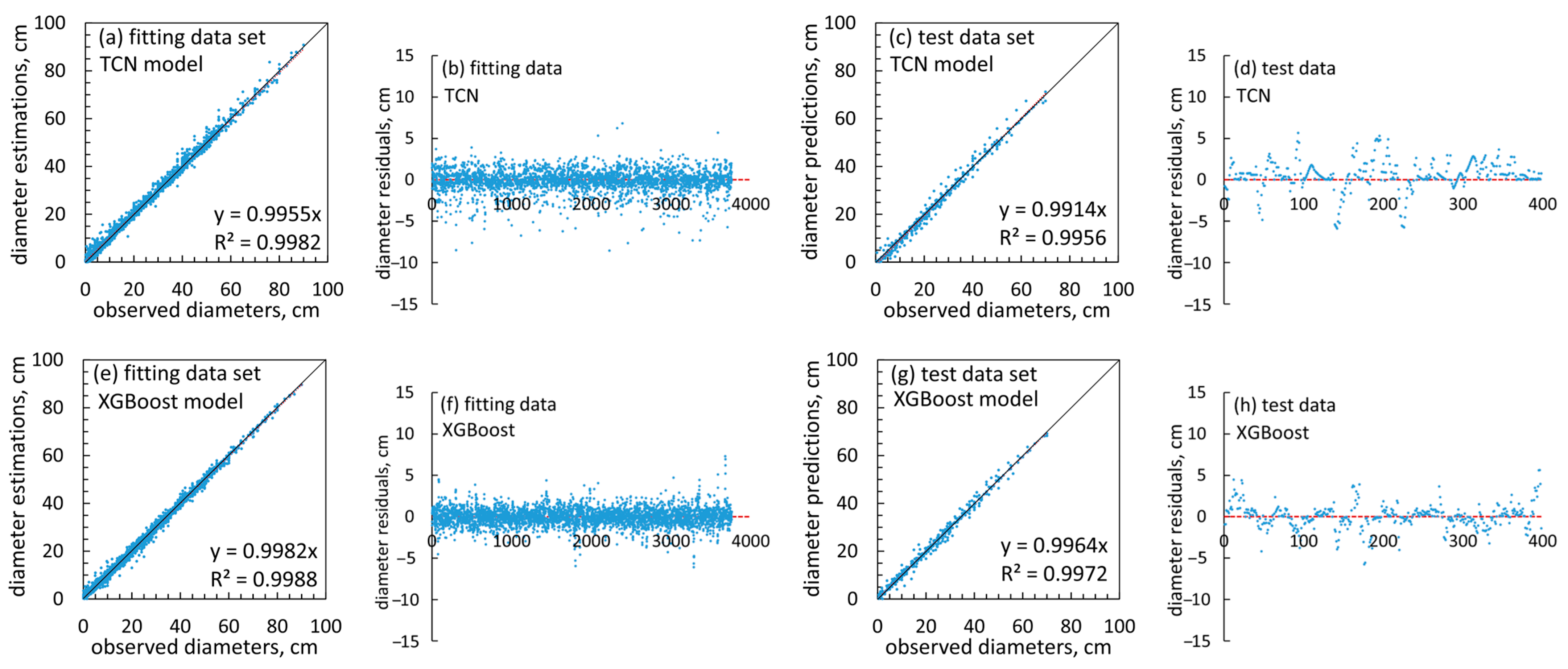
The performance scatter plots of both modeling approaches (estimations to a known data set (fitting) and predictions to a different data set (test)) versus the observed diameter values at different stem heights, along with the corresponding residuals, are shown in Figure 6.

As can be seen (Figure 6), both TCN and XGBoost models’ estimations (Figure 6a,e) and predictions (Figure 6c,g) align closely to the 45-degree line, indicating a strong adaptation to the fitting data and strong generalization ability according to the test data set. However, deviations are observed without any visible trend or significant heteroscedasticity, indicating very good model performance, with higher performance for the XGBoost model. According to the residual plots of the TCN (Figure 6b,d) and XGBoost (Figure 6f,h) models, both show random scatter around zero with no obvious structures or outliers.

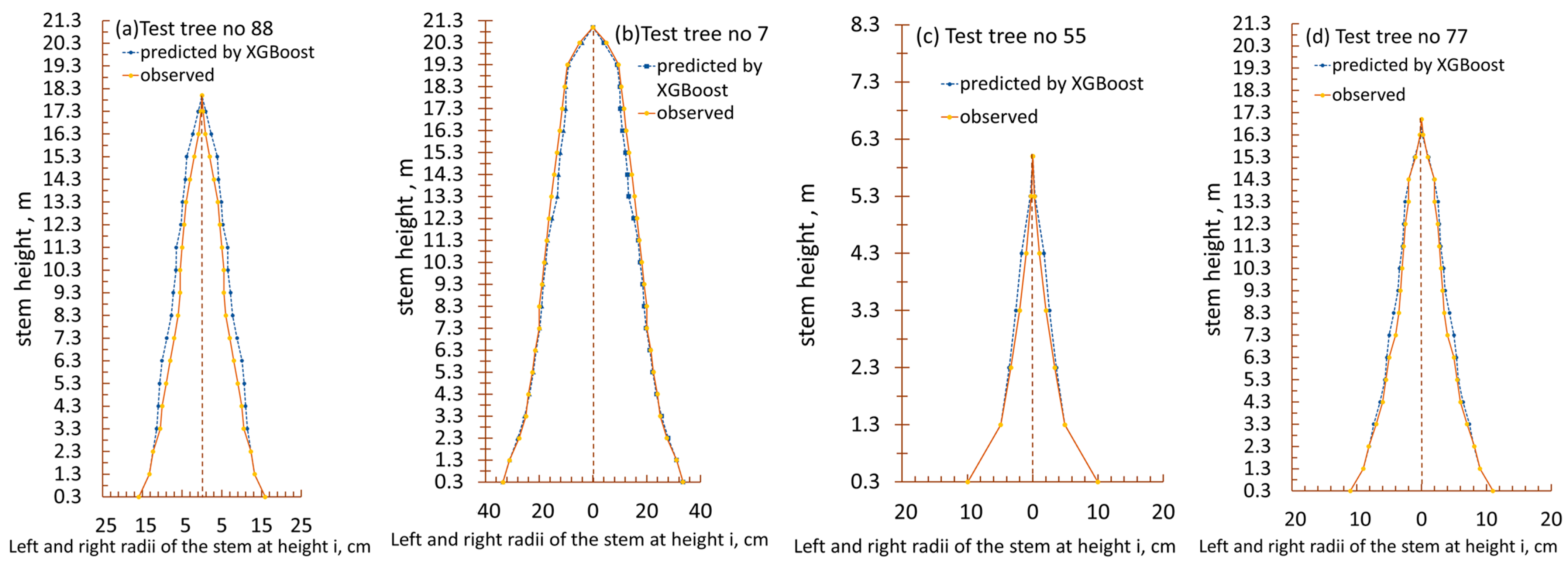
XGBoost constructed model appears to outperform in estimating and predicting diameters along the tree stem, achieving the highest performance with consistent results across both small and large diameters. Indicatively, the performance of the XGBoost model in accurately predicting stem diameters at different growth stages for four trees in the test dataset is shown in Figure 7. The XGBoost model’s predicted diameters performed better near the ground, while small errors were observed in predicting middle and upper-stem diameters (Figure 7). Since the largest diameters and, consequently, the most significant proportion of merchantable wood are located near the ground rather than in the upper stem, the discrepancies observed in middle and upper-stem diameter predictions are not considered significant.

Overall, the stem diameter estimation and prediction errors (Table 3) obtained from the XGBoost model (Table 2) indicate that the model performs adequately, supporting its suitability as an accurate and reliable tool for predicting stem diameters in standing trees.

3.2. Total and Segmented Stem Volume Prediction

The machine learning models presented in Table 2 were applied to generate stem diameter estimates and predictions, which were then used to compute total and segmented stem volumes. Observed stem volumes were calculated using Smalian’s formula based on measured stem diameters. Subsequently, the same formula was applied to predict total and 1 m segment volumes using the models’ estimated and predicted stem diameters.

Figure 8 presents the predicted total stem volume versus the observed total stem volume across different observed total tree stem volume ranges for the fitting and test data sets. According to the first range defined by observed total stem volume < 1.0 m³ (Figure 8a), the RMSE% was 4.10% and 3.71% of the mean observed stem volume for the volume predictions based on the TCN and XGBoost models, respectively. For the second class, corresponding to observed volumes in the range [1.0, 2.0) m³ (Figure 8b), the RMSE% was 2.64% and 2.01% of the mean observed stem volume for the volume predictions based on the TCN and the XGBoost models, respectively. A similar pattern has been observed for the fourth class, corresponding to observed volumes in the range [3.0, 6.0) m³ (Figure 8d), where the XGBoost model’s use, produced results that also clearly outperformed, producing a RMSE% value of 1.81%. However, for the third class ([2.0, 3.0) m³; Figure 8c), the XGBoost-based diameter predictions did not yield the highest accuracy. Within this volume range of the fitting data set, the RMSE% was 1.47% with TCN-estimated diameters, compared to 1.74% with XGBoost-estimated diameters, which is a slightly higher value.

Using the XGBoost-generated diameters also resulted in better agreement with the test data set (Figure 8e,f) for both evaluated volume classes (<1.0 m³ and [1.0–4.3) m³). The RMSE% values obtained with the TCN model were 9.53% and 6.94% for these respective classes (Figure 8e,f), whereas the corresponding values for the XGBoost model were 7.94% and 3.73%.

The evaluation metrics for total stem volume predictions using both machine learning-constructed models (Table 2) across different total stem volume ranges are presented in

Table 4. Evaluation metrics for the total stem volume predictions using both machine learning constructed models, in different ranges, for the fitting and the test data sets.

	Models
	TCN			XGBoost
	RMSE, m3	R	AAE, m3	RMSE, m3	R	AAE, m3
range, m3	Fitting data set
<1.0	0.0179	0.9984	0.0130	0.0162	0.9993	0.0087
[1.0–2.0)	0.0402	0.9917	0.0284	0.0306	0.9930	0.0192
[2.0–3.0)	0.0356	0.9942	0.0262	0.0422	0.9883	0.0252
[3.0–6.0)	0.6573	0.9958	0.0840	0.0496	0.9997	0.0332
	Test data set
<1.0	0.0389	0.9968	0.0314	0.0324	0.9939	0.0255
[1.0–4.3)	0.1697	0.9835	0.1267	0.0910	0.9952	0.0820

.

As can be observed (Table 4), for all ranges, the absolute average error of the predicted total stem volume was lower for the case of the stem diameters based on the XGBoost model, for both the fitting and the test data sets. At the same time, the RMSE values were lower for the XGBoost model, except for the volume range of 2.0 to 3.0 m³, for the fitting data set. For this range, the RMSE value was slightly higher by 0.0066 m³. Generally, both approaches yielded adequate and reliable results, which were highly correlated with the calculated volume based on the observed stem diameters.

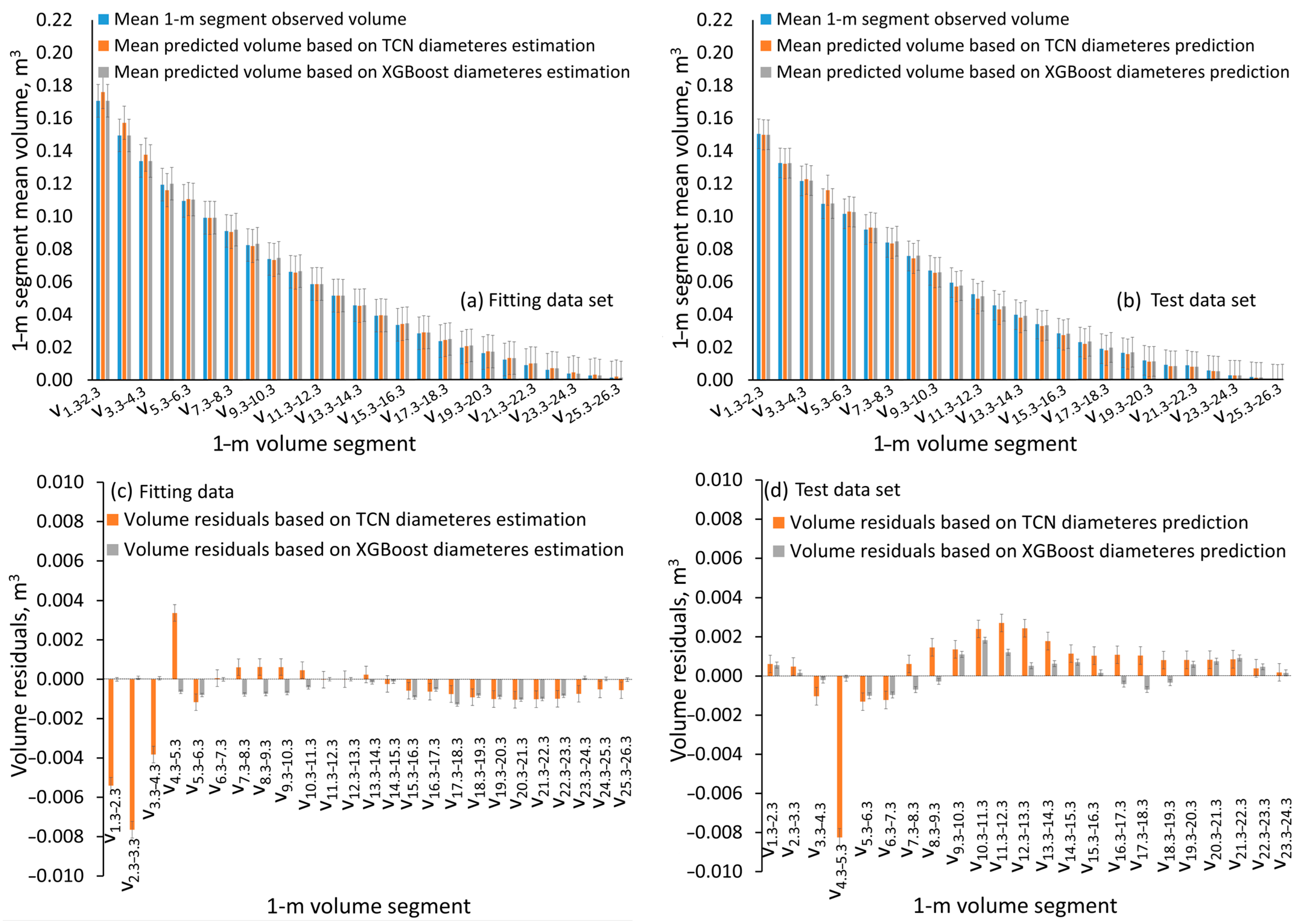
Subsequently, to assess the predictive accuracy of the segmented stem volumes, the estimated 1 m segment mean volumes were compared with the corresponding observed segment mean volumes. These comparisons were based on stem diameters estimated and predicted by the TCN and XGBoost models. Figure 9a,b show the mean predicted and mean observed 1 m segment volumes for both the fitting and test data sets, respectively, beginning at 1.3 m above ground level.

The volume of the first segment (between d_0.3 and d_1.3) was computed using the observed diameters at these heights, as these measurements were required as input variables for both the TCN and XGBoost models. As a result, diameters measured close to the ground are necessary for the operational use of the volume-prediction system.

Figure 9c,d show differences in mean segmental volume predictions and observed values. In both figures, the residuals associated with the XGBoost-based diameter estimates were, in most cases, smaller than those produced by the TCN model. Moreover, the XGBoost model exhibited notably higher accuracy in the lower sections of the tree stem, where diameters are largest, and the highest-quality, most commercially valuable wood is typically found. Finally, the XGBoost model demonstrated better generalization performance (Figure 9b,d).

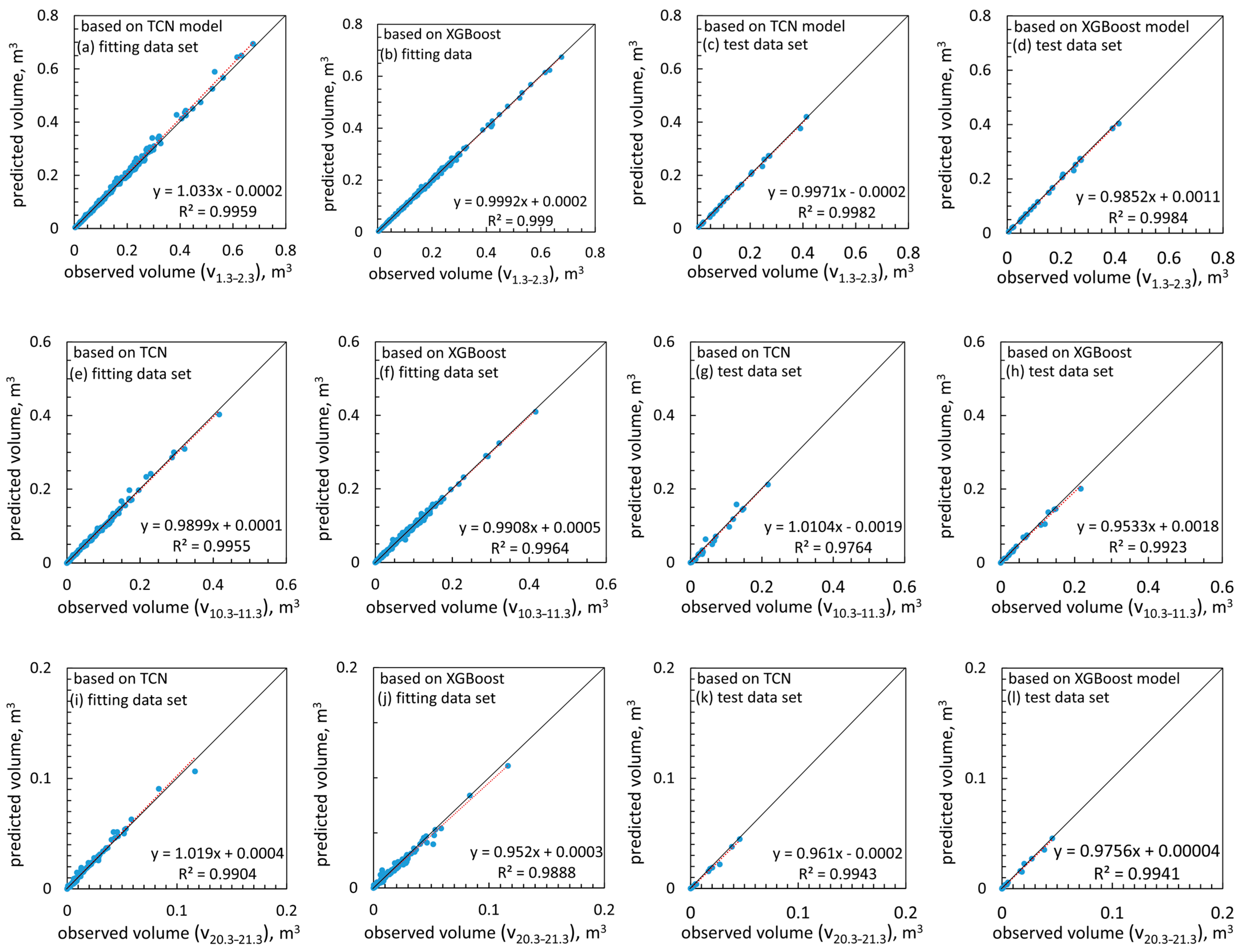
To present the specific volume predictions adapted to each segment of the sample trees, 45-degree line plots were produced for the fitting and test data sets. Representative plots for the observed volume segments v_1.3–2.3, v_10.3–11.3, and v_20.3–21.3 are shown in Figure 10.

The regression lines for both the fitting and test data sets (Figure 10), based on both modeling approaches, lie very close to the red dashed 1:1 line, indicating that the estimates and predictions from both models’ diameters are highly consistent with the actual measurements. Slight deviations are visible, but they are minor compared to the overall trend. As observed, the stem diameters derived by the XGBoost model performed better, with a clearly higher degree of adaptation at low and medium stem heights (Figure 10a–h). According to the higher stem segment volume between 20.3 m and 21.3 m, and for the fitting data set, the segmented volume based on the TCN model’s diameters seemed to achieve higher, though close, precision than that based on the XGBoost model’s diameters. (Figure 10i,j). At the same time, both approaches demonstrated strong generalization on the new test dataset (Figure 10k,l).

4. Discussion

Due to its importance, tree taper prediction has been faced through many modeling procedures, from simple continuous functions for the total stem [59], to segmented polynomial functions [7], to models with the use of exponent on the diameter–height relationship which allowed the model change along the stem [8], and to compatible taper-volume systems [60]. Lately, mixed-effects models have been used to handle potential correlation and heteroscedasticity in the data [14]. Although these modeling methodologies have been found adequate for tree taper estimation, all have two basic disadvantages that make proper model construction time-consuming and difficult. The first is that all require a predetermined model form, which is challenging to select, and the second is that many statistical assumptions must be carefully checked to construct a reliable model.

Because machine learning methods are non-parametric and can learn effectively from ground-truth data, they offer strong potential for predicting difficult-to-measure field biometric variables, such as tree stem diameters. This potential has motivated investigations into these methods and algorithms to evaluate their effectiveness in practical forestry applications. Specifically, taper modeling has progressed to the exploration and use of promising new machine learning approaches to overcome challenges and improve accuracy beyond the capabilities of standard regression procedures. A recent review of taper modeling methodologies [5], including machine learning approaches, concluded that, to date, developing taper functions remains challenging and warrants further exploration. According to Crimean pine trees (Pinus nigra J.F. Arnold subsp. pallasiana [Lamb.] Holmboe), an artificial neural network approach was found to be successful for taper modeling and superior to Max-Burkhart’s equation [61]. The applicability of XGBoost and random forest machine learning approaches was tested in taper modeling and compared with standard regression procedures by Sağlam [24], who concluded that the XGBoost model outperformed for Turkish pine (Pinus brutia) stands. In the same direction, a comparative analysis was applied using a random sample of black pine (Pinus nigra) stands [40] to evaluate standard non-linear regression and machine learning approaches. The XGBoost method demonstrated superior performance in estimating and predicting total tree stem volumes. To establish a baseline related to accuracy, the best-fitting standard non-linear regression model for the same area achieved a root mean square error percentage (RMSE%) of 9.35% for total tree stem volume [40]. In contrast, the XGBoost model in the current study achieved an RMSE% of 2.99% for the same metric and for the total tree stem volume. The combined findings from the current and previous studies in this forest area underscore the significant improvements provided by the XGBoost machine learning approach for estimating stem volume in Pinus nigra trees and stands.

Lately, a few attempts have been made to model tree taper as a sequence of diameters along the stem [28,61]. In these attempts, deep learning for sequential data was borrowed from time-series and effectively used, including recurrent neural networks to successfully model double bark thickness along the stem for Scots pine (Pinus sylvestris) and common oak (Quercus robur L.) trees [28], and a long short-term memory approach for successfully learning the tree taper, optimizing in this way the forest management decisions [62]. In this regard, a deep learning architecture based on Temporal Convolutional Networks (TCNs), specifically designed to model sequential data, was applied to predict taper in Pinus nigra trees. In parallel, the XGBoost algorithm, recently shown to be highly effective for taper modeling, was employed as a robust gradient-boosted tree ensemble method that approached the taper estimation problem from a fundamentally different analytical perspective.

According to this study’s results, tree stem diameters were found to be non-stationary, with a systematic taper trend (Figure 5). The ACF applied to the detrended residuals showed that the most significant trend-related correlation occurred at lag 1, with stem height 1.3 m from the ground (Figure 5). At the same time, the autocorrelation was non-significant for the remaining diameters measured at 1 m above breast height. Considering that the stem is a spatially ordered biological structure in which local deviations are hierarchically integrated along the bole, this supports the use of both the selected TCN and XGBoost models, in the sense that weak linear autocorrelation does not imply the absence of meaningful structural dependence exploitable by sequence models, such as TCN. On the one hand, TCN considers ordering and adjacency, even when correlation is weak, and shows the ability to model how small-scale deviations combine into larger-scale form. It does not require stationarity, can effectively handle both short- and long-range dependencies, and is well suited to the nonlinear nature of tree taper. On the other hand, XGBoost treats taper modeling as a non-sequential, nonlinear estimation and prediction problem. The ground-truth data showed a deterministic taper trend with minimal autocorrelation, making tree-based regression highly suitable.

According to the TCN model, both causality and a dilation rate of 1 were used during training. These settings were selected for the model’s training to consider only current and previous stem diameters, and to set the spacing between kernel elements to 1. These arrangements reinforce the practical importance of the final constructed model. The optimal value of the kernel (Table 2) showed that the two previous steps in diameters were the best choice, meaning that the configuration of value of the diameter at any 1 m height from 1.3 m, initially based on the d_0.3 and d_1.3, meaning that these observed diameters are required for the prediction chain of the remaining diameters along the stem. This finding may be valuable for future work, even with alternative modeling approaches, as it highlights the importance of diameter measurements taken at closely spaced heights to the ground. If further validated, this result could reduce the number of field measurements required in similar modeling applications.

While TCNs model spatial dependencies, XGBoost can serve as a strong alternative for summarizing spatial patterns, such as stem diameter growth rates. This fact allows XGBoost to approximate spatial dynamics without deep learning. Both modeling approaches used the same input information, so the practical importance of the final constructed model is the same for both alternatives. Consequently, the d_0.3, the d_1.3, and the predetermined stem diameter height to be predicted were the input variables of the XGBoost model’s input layer. The best-fitted XGBoost model (Table 2) was finally a model with a substantial individual impact of each decision tree (lr = 0.28), enough complexity to capture nonlinear patterns avoiding overfitting (n_dt = 185, d_max = 5, γ = 0.11, and early stopping), and capacity to capture fine-grained patterns (mcw = 1).

Considering the evaluation metrics (Table 3) of the best-fitting constructed models in Table 2, both approaches demonstrated high and close adaptability to the fitting data set and, at the same time, acceptable generalization performance, with the XGBoost model consistently outperforming in tree stem diameter estimation and prediction. A reason for the observed outperformance of the XGBoost-developed model might be the weak linear dependence of the detrended residuals across height intervals (Figure 5), a condition that could favor XGBoost over TCN. The XGBoost model generalized better for diameters near the ground than for higher ones (Figure 7). This could happen because the observed diameters of stems within the crown are often difficult to measure accurately on standing trees, making it challenging to train the model to these specific diameters.

Accurate prediction of tree taper from stem diameter configuration could be beneficial for predicting total and segmented stem volume. Considering the findings on the use of the derived stem diameters by the two modeling approaches in stem volume prediction, this benefit can be ascertained.

The total stem volume prediction across different stem volume ranges (Figure 8, Table 4) yielded RMSE (RMSE%) values lower than 0.6573 (4.10%) and 0.1697 (9.53%) of the observed stem volume for the fitting and test data sets, respectively. Specifically, the use of the XGBoost model reduces the total volume prediction error, producing RMSE (RMSE%) values lower than 0.0496 (3.71%) and 0.0910 (7.94%) of all ranges of the observed stem volume for the fitting and test data sets, which is a significant improvement in accuracy for both data sets.

Based on the segmented stem volumes (Figure 9 and Figure 10), the 1 m volumes derived from the XGBoost-predicted diameters were the most accurate and consistent across the majority of segments. For the fitting dataset, the highest height-related accuracy occurred below 11.3 m, corresponding to the lower stem section that contributes most of the high-value sawn timber (Figure 9a,c). A similar pattern was observed in the test dataset, confirming both the suitability and the strong generalization performance of the XGBoost model across nearly all 1 m segments.

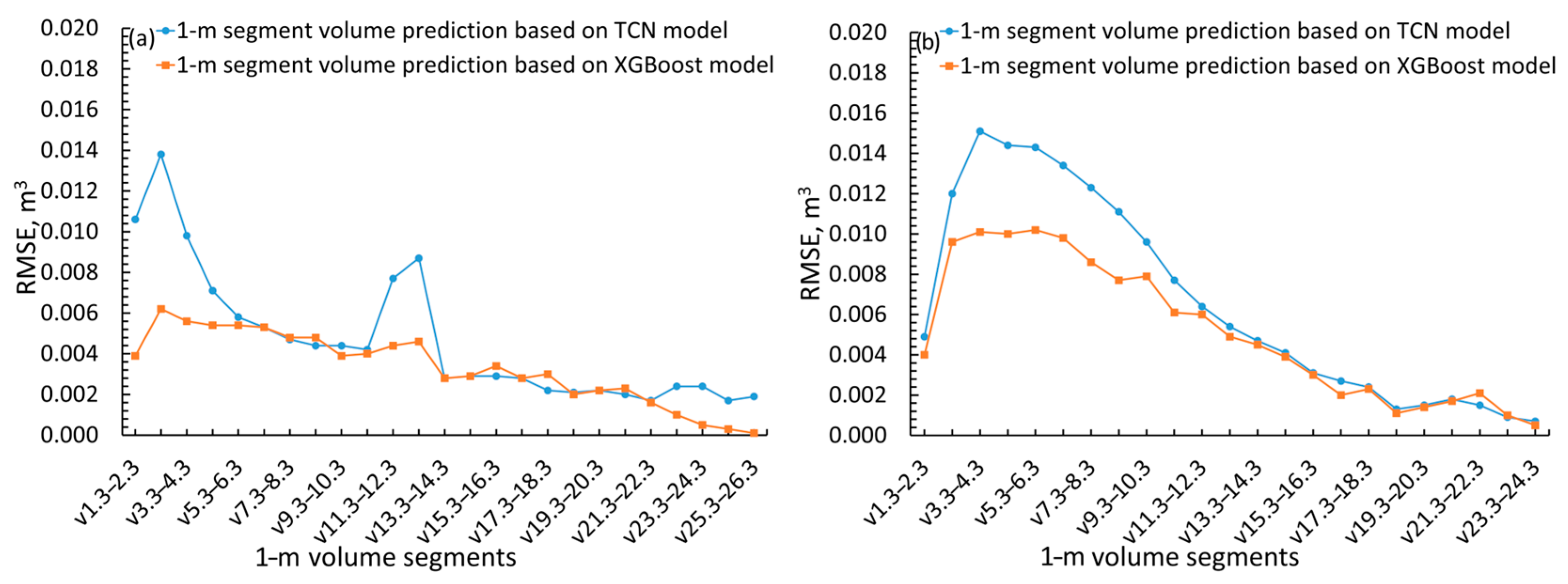
Furthermore, the RMSE patterns between observed and predicted values were closely aligned for both the fitting and test datasets (Figure 11a,b). The deviations from the general RMSE trend are shown in Figure 11. These deviations may reflect biological variation in the stem across different heights. Generally, the RMSE values for each 1 m segment showed the XGBoost model’s strong ability to capture the general pattern of stem growth.

While both modeling approaches have significant advantages, such as their non-parametric nature and strong ability to learn from ground-truth data, they also have weaknesses that should be considered before use. TCNs are designed for sequential data; when applied outside this context, their performance degrades and they require more computational resources and time, typically longer than for XGBoost. However, hyperparameter optimization for both approaches requires effort through trials and cross-validation procedures. In addition, while XGBoost requires manually specified features, TCN offers the significant advantage of selecting the optimal sequence depth, with practical value. Both models demonstrated their ability to accurately predict stem diameters along the stem, resulting in highly accurate stem volume prediction. The decision on which methodology to use should be based on the problem’s nature and structure.

Overall, the results confirm the suitability of both methods, with XGBoost achieving superior performance. Future research has to investigate further these modeling approaches across additional species and forest areas, to strengthen the research base supporting informed methodological recommendations.

5. Conclusions

Modeling tree taper presents a significant challenge in forestry. This study analyzes the stem-diameter patterns of black pine (Pinus nigra) in the Karya forest on Mount Olympus. Two machine learning methods, the Temporal Convolutional Network (TCN) and Extreme Gradient Boosting (XGBoost), were evaluated for their effectiveness in modeling stem profiles. The objective was to identify a reliable and efficient approach for predicting stem sectional volume using minimal field measurements.

The results indicated that the diameters of Pinus nigra trees were primarily influenced by a systematic taper trend, with trend-related correlation observed only at lag 1. This weak linear autocorrelation across height intervals suggests the presence of short-range structured variation.

The comparative analysis of TCN- and XGBoost-constructed models showed their strong ability to capture the taper trend of the trees, estimating and predicting the diameters along the tree stem with high accuracy.

XGBoost demonstrated strong suitability for the available dataset by effectively summarizing its spatial structure. This approach substantially improved the accuracy of sectional stem-volume predictions based on stump and breast-height diameter measurements, yielding significant practical outcomes.

References

1. Trincado, G.; Burkhart, H.E. A generalized approach for modeling and localizing stem profile curves. For. Sci. 2006, 52, 670–682. [Google Scholar] [CrossRef]
2. West, P.W. Tree and Forest Measurement, 3rd ed.; Springer: Cham, Switzerland, 2015. [Google Scholar] [CrossRef]
3. Kershaw, J.A., Jr.; Ducey, M.J.; Beers, T.W.; Husch, B. Forest Mensuration, 5th ed.; John Wiley & Sons Ltd.: Chichester, UK, 2017. [Google Scholar]
4. Burkhart, H.E.; Tomé, M. Modeling Forest Trees and Stands; Springer Science & Business Media: Berlin, Germany, 2012. [Google Scholar]
5. Salekin, S.; Catalán, C.H.; Boczniewicz, D.; Phiri, D.; Morgenroth, J.; Meason, D.F.; Mason, E.G. Global Tree Taper Modelling: A Review of Applications, Methods, Functions, and Their Parameters. Forests 2021, 12, 913. [Google Scholar] [CrossRef]
6. Demaerschalk, J.P. Converting volume equations to compatible taper equations. For. Sci. 1972, 18, 241–245. [Google Scholar] [CrossRef]
7. Max, T.A.; Burkhart, H.E. Segmented polynomial regression applied to taper equations. For. Sci. 1976, 18, 283–289. [Google Scholar] [CrossRef]
8. Kozak, A. A variable-exponent taper equation. Can. J. For. Res. 1988, 18, 1363–1368. [Google Scholar] [CrossRef]
9. Kozak, A. My last words on taper equations. For. Chron. 2004, 80, 507–515. [Google Scholar] [CrossRef]
10. Lejeune, G.; Ung, C.H.; Fortin, M.; Guo, X.J.; Lampert, M.C.; Ruel, J.C. A simple stem taper model with mixed effects for boreal black spruce. Eur. J. Forest Res. 2009, 128, 505–513. [Google Scholar] [CrossRef]
11. Özçelik, R.; Alkan, O. Fitting and calibrating a mixed-effects segmented taper model for brutian pine. Cerne 2020, 26, 464–473. [Google Scholar] [CrossRef]
12. Li, D.; Guo, H.; Jia, W.; Wang, F. Analysis of Taper Functions for Larix olgensis Using Mixed Models and TLS. Forests 2021, 12, 196. [Google Scholar] [CrossRef]
13. Draper, N.R.; Smith, H. Applied Regression Analysis, 3rd ed.; Wiley: New York, NY, USA, 1998. [Google Scholar]
14. Özçelik, R.; Cao, Q.V.; Trincado, G.; Göçer, N. Predicting tree height from tree diameter and dominant height using mixed-effects and quantile regression models for two species in Turkey. For. Ecol. Manag. 2018, 419–420, 240–248. [Google Scholar] [CrossRef]
15. Diamantopoulou, M.J.; Özçelik, R.; Eler, Ü.; Koparan, B. From Regression to Machine Learning: Modeling Height–Diameter Relationships in Crimean Juniper Stands Without Calibration Overhead. Forests 2025, 16, 972. [Google Scholar] [CrossRef]
16. Diamantopoulou, M.J. Assessing a reliable modeling approach of features of trees through neural network models for sustainable forests. Sustain. Comput. Inform. Syst. 2012, 2, 190–197. [Google Scholar] [CrossRef]
17. Zhou, R.; Wu, D.; Zhou, R.; Fang, L.; Zheng, X.; Lou, X. Estimation of DBH at Forest Stand Level Based on Multi-Parameters and Generalized Regression Neural Network. Forests 2019, 10, 778. [Google Scholar] [CrossRef]
18. Ercanlı, İ. Innovative deep learning artificial intelligence applications for predicting relationships between individual tree height and diameter at breast height. For. Ecosyst. 2020, 7, 12. [Google Scholar] [CrossRef]
19. Sun, Y.; Ao, Z.; Jia, W.; Chen, Y.; Xu, K. A geographically weighted deep neural network model for research on the spatial distribution of the down dead wood volume in Liangshui National Nature Reserve (China). iForest 2021, 14, 353. [Google Scholar] [CrossRef]
20. Nunes, M.H.; Görgens, E.B. Artificial Intelligence Procedures for Tree Taper Estimation within a Complex Vegetation Mosaic in Brazil. PLoS ONE 2016, 11, e0154738. [Google Scholar] [CrossRef]
21. Özçelik, R.; Diamantopoulou, M.J.; Trincado, G. Evaluation of potential modeling approaches for Scots pine stem diameter prediction in north-eastern Turkey. Comput. Electron. Agric. 2019, 162, 773–782. [Google Scholar] [CrossRef]
22. Sandoval, S.; Acuña, E. Stem Taper Estimation Using Artificial Neural Networks for Nothofagus Trees in Natural Forest. Forests 2022, 13, 2143. [Google Scholar] [CrossRef]
23. Ko, C.; Kang, J.; Lim, C.; Kim, D.; Lee, M. Application of Machine Learning Models in the Estimation of Quercus mongolica Stem Profiles. Forests 2025, 16, 1138. [Google Scholar] [CrossRef]
24. Sağlam, F. Machine learning-based stem taper model: A case study with Brutian pine. Front. For. Glob. Chang. 2025, 8, 1609549. [Google Scholar] [CrossRef]
25. Diamantopoulou, M.J.; Özçelik, R.; Kalkanli Genç, Ş. Evaluation of the random forest regression machine learning technique as an alternative to ecoregional based regression taper modelling. Comput. Electron. Agric. 2025, 239, 110964. [Google Scholar] [CrossRef]
26. Van Laar, A.; Akça, A. Forest Mensuration; Springer: Dordrecht, The Netherlands, 2007. [Google Scholar]
27. Myers, R.H. Classical and Modern Regression with Applications, 2nd ed.; PWS-Kent: Boston, MA, USA, 1990. [Google Scholar]
28. Cywicka, D.; Jakóbik, A.; Socha, J.; Pasichnyk, D.; Widlak, A. Modelling bark thickness for Scots pine (Pinus sylvestris L.) and common oak (Quercus robur L.) with recurrent neural networks. PLoS ONE 2022, 17, e0276798. [Google Scholar] [CrossRef] [PubMed]
29. Luković, M.; Zweifel, R.; Thiry, G.; Zhang, C.; Schubert, M. Reconstructing radial stem size changes of trees with machine. J. R. Soc. Interface 2022, 19, 20220349. [Google Scholar] [CrossRef] [PubMed]
30. Amir, A.; Butt, M. Improved sap flow prediction: A comparative deep learning study based on LSTM, BiLSTM, LRCN, and GRU with stem diameter data. Smart Agric. Technol. 2025, 12, 101105. [Google Scholar] [CrossRef]
31. Pelletier, C.; Webb, G.I.; Petitjean, F. Temporal Convolutional Neural Network for the Classification of Satellite Image Time Series. Remote Sens. 2019, 11, 523. [Google Scholar] [CrossRef]
32. Kantavichai, R.; Turnblom, E.C. Identifying non-thrive trees and predicting wood density from resistograph using temporal convolution network. For. Sci. Technol. 2022, 18, 144–149. [Google Scholar] [CrossRef]
33. Duan, R.; Huang, C.; Dou, P.; Hou, J.; Zhang, Y.; Gu, J. Fine-scale forest classification with multi-temporal sentinel-1/2 imagery using a temporal convolutional neural network. Int. J. Digit. Earth 2025, 18, 2457953. [Google Scholar] [CrossRef]
34. Liu, G.; Wang, J.; Dong, P.; Chen, Y.; Liu, Z. Estimating Individual Tree Height and Diameter at Breast Height (DBH) from Terrestrial Laser Scanning (TLS) Data at Plot Level. Forests 2018, 9, 398. [Google Scholar] [CrossRef]
35. Ye, N.; Mason, E.; Xu, C.; Morgenroth, J. Estimating individual tree DBH and biomass of durable Eucalyptus using UAV LiDAR. Ecol. Inform. 2025, 89, 103169. [Google Scholar] [CrossRef]
36. Espíndola, R.P.; Picanço, M.M.; de Andrade, L.P.; Ebecken, N.F.F. Applications of Machine Learning Methods in Sustainable Forest Management. Climate 2025, 13, 159. [Google Scholar] [CrossRef]
37. Subedi, B.; Morneau, A.; LeBel, L.; Gautam, S.; Cyr, G.; Tremblay, R.; Carle, J.-F. An XGBoost-Based Machine Learning Approach to Simulate Carbon Metrics for Forest Harvest Planning. Sustainability 2025, 17, 5454. [Google Scholar] [CrossRef]
38. Ampatzidis, D.; Moschopoulos, G.; Mouratidis, A.; Styllas, M.; Tsimerikas, A.; Deligiannis, V.-K.; Voutsis, N.; Perivolioti, T.-M.; Vergos, G.S.; Plachtova, A. Revisiting the determination of Mount Olympus Height (Greece). J. Mt. Sci. 2023, 20, 1026–1034. [Google Scholar] [CrossRef]
39. Forest Service of Elassona, Greece. Forest Management Plan for the Public Forest of Karya, Management Period 2014–2023; Municipality of Elassona, Forest Service of Elassona: Elassona, Greece, 2015. (In Greek) [Google Scholar]
40. Diamantopoulou, M.J.; Georgakis, A. Improving European Black Pine Stem Volume Prediction Using Machine Learning Models with Easily Accessible Field Measurements. Forests 2024, 15, 2251. [Google Scholar] [CrossRef]
41. Roesch, F.A. Adaptive cluster sampling for forest inventories. For. Sci. 1993, 39, 655–669. [Google Scholar] [CrossRef]
42. Rogerson, P.A. Spatial Sampling. In Encyclopedia of Social Measurement; Kempf-Leonard, Ed.; Elsevier Inc.: Amsterdam, The Netherlands, 2005; Volume 3, pp. 633–638. [Google Scholar]
43. IBM Corp. IBM SPSS Statistics for Windows; Version 29.01; Released 2023; IBM Corp.: Armonk, NY, USA, 2023. [Google Scholar]
44. Diamantopoulou, M.J. Filling gaps in diameter measurements on standing tree boles in the urban forest of Thessaloniki, Greece. Environ. Model. Softw. 2010, 25, 1857–1865. [Google Scholar] [CrossRef]
45. Shumway, R.H.; Stoffer, D.S. Time Series Analysis and Its Applications: With R Examples, 4th ed.; Springer: Cham, Switzerland, 2017. [Google Scholar] [CrossRef]
46. Wold, H.O.A. A Study in the Analysis of Stationary Time Series, 2nd ed.; Almqvist & Wiksell: Stockholm, Sweden, 1956. [Google Scholar] [CrossRef]
47. Dickey, D.A.; Fuller, W.A. Likelihood Ratio Statistics for Autoregressive Time Series with a Unit Root. Econometrica 1981, 49, 1057–1072. [Google Scholar] [CrossRef]
48. Kwiatkowski, D.; Phillips, P.C.B.; Schmidt, P.; Shin, Y. Testing the null hypothesis of stationarity against the alternative of a unit root. J. Econom. 1992, 54, 159–178. [Google Scholar] [CrossRef]
49. Berendt, F.; de Miguel-Diez, F.; Wallor, E.; Blasko, L.; Cremer, T. Comparison of different approaches to estimate bark volume of industrial wood at disc and log scale. Sci. Rep. 2021, 11, 15630. [Google Scholar] [CrossRef]
50. Burkhart, H.E.; Avery, T.E.; Bullock, B.P. Forest Measurements, 6th ed.; Waveland Pr Inc.: Long Grove, IL, USA, 2018. [Google Scholar]
51. Olson, D.L.; Delen, D. Advanced Data Mining Techniques; Springer Science & Business Media: Berlin/Heidelberg, Germany, 2008. [Google Scholar]
52. Lea, C.; Vidal, R.; Reiter, A.; Hager, G.D. Temporal Convolutional Networks: A Unified Approach to Action Segmentation. In Computer Vision—ECCV 2016 Workshops; Lecture Notes in Computer Science; Hua, G., Jégou, H., Eds.; Springer: Cham, Switzerland, 2016; Volume 9915, pp. 47–54. [Google Scholar] [CrossRef]
53. Dubey, S.R.; Singh, S.K.; Chaudhuri, B.B. Activation functions in deep learning: A comprehensive survey and benchmark. Neurocomputing 2022, 503, 92–108. [Google Scholar] [CrossRef]
54. Pedregosa, F.; Varoquaux, G.; Gramfort, A.; Michel, V.; Thirion, B.; Grisel, O.; Blondel, M.; Prettenhofer, P.; Weiss, R.; Dubourg, V.; et al. Scikit-learn: Machine learning in Python. J. Mach. Learn. Res. 2011, 12, 2825–2830. [Google Scholar]
55. Python Software Foundation. Python Language Reference, Version 3.13; Python Software Foundation: Wilmington, DE, USA, 2023. Available online: https://docs.python.org/3.13/index.html (accessed on 11 October 2024).
56. Chen, T.; Guestrin, C. XGBoost: A scalable tree boosting system. In Proceedings of the KDD ’16: 22nd ACM SIGKDD International Conference on Knowledge Discovery and Data Mining, San Francisco, CA, USA, 13–17 August 2016; pp. 785–794. [Google Scholar] [CrossRef]
57. Bergstra, J.; Bardenet, R.; Bengio, Y.; Kégl, B. Algorithms for Hyper-Parameter Optimization. In Proceedings of the 24th International Conference on Neural Information Processing Systems, Granada, Spain, 12–15 December 2011; pp. 2546–2554. [Google Scholar]
58. Watanabe, S. Tree-Structured Parzen Estimator: Understanding Its Algorithm Components and Their Roles for Better Empirical Performance. arXiv 2025, arXiv:2304.11127. [Google Scholar] [CrossRef]
59. Ormerod, D.W. A simple bole model. For. Chron. 1973, 49, 136–138. [Google Scholar] [CrossRef]
60. Özçelik, R.; Brooks, J.R. Compatible volume and taper models for economically important tree species of Turkey. Ann. For. Sci. 2012, 69, 105–118. [Google Scholar] [CrossRef]
61. Șahin, A. Analyzing regression models and multi-layer artificial neural network models for estimating taper and tree volume in Crimean pine forests. iForest 2024, 17, 36–44. [Google Scholar] [CrossRef]
62. Schmiedel, S. Stochastic stem bucking using mixture density neural networks. arXiv 2024, arXiv:2407.00510. [Google Scholar] [CrossRef]
Figure 1. Study area located in Karya Forest on Mount Olympus.
Forests 17 00054 g001
Figure 2. (a) Mean and (b) variance diameter plots.
Forests 17 00054 g002
Figure 3. Indicative splines fit related to four (ad) different tree diameter profiles.
Forests 17 00054 g003
Figure 4. Data division flowchart.
Forests 17 00054 g004
Figure 5. Autocorrelation mean trend of fitting trees’ detrended residuals per height lag.
Forests 17 00054 g005
Figure 6. Scatter plots of estimations (a,e) and predictions (c,g) versus the observed diameter values, and the corresponding residuals (b,d,f,h) for the TCN (ad) and the XGBoost (eh) models.
Forests 17 00054 g006
Figure 7. Predicted stem diameters from the XGBoost model for four test-set trees (ad) differing in total height.
Forests 17 00054 g007
Figure 8. Plots of estimated (ad) and predicted (e,f) total stem volumes versus the observed total stem volumes for different volume ranges.
Forests 17 00054 g008aForests 17 00054 g008b
Figure 9. Comparison of mean predicted and mean observed 1 m stem-segment volumes for the (a) fitting and (b) test data sets. Predictions are based on stem diameters (a) estimated and (b) predicted by the TCN and XGBoost models. Volumes are shown for segments beginning at 1.3 m above ground level. Volume residuals derived from (c) estimated and (d) predicted by the TCN and XGBoost models stem diameters.
Forests 17 00054 g009
Figure 10. 45-degree line plots for the fitting (a,b,e,f,i,j) and the test data sets (c,d,g,h,k,l) for the observed volume segments of v1.3–2.3 (ad), v10.3–11.3 (eh) and v20.3–21.3 (il) based on TCN (a,c,e,g,i,k) and XGBoost (b,d,f,h,j,l) modeling approaches.
Forests 17 00054 g010
Figure 11. Root mean square error values between predicted and observed 1 m stem-segment volumes for the (a) fitting and (b) test data sets, based on both modeling approaches.
Forests 17 00054 g011