Article

Temporal and Spatial Variations of Energy Exchanging Under Varying Urban Riparian Forest Plant Communities: A Case Study of Shanghai, China

1
School of Design, Shanghai Jiao Tong University, Shanghai 200240, China
2
School of Agriculture and Biology, Shanghai Jiao Tong University, Shanghai 200240, China
3
Lijiang Scenic Area Strategic Development Office, The Lijiang River Tourist Attractions Department, Guilin 541001, China
*
Author to whom correspondence should be addressed.
Forests 2025, 16(9), 1466; https://doi.org/10.3390/f16091466
Submission received: 18 July 2025 / Revised: 12 September 2025 / Accepted: 12 September 2025 / Published: 15 September 2025
(This article belongs to the Section Urban Forestry)

Abstract

Urban riparian areas serve as vital blue-green infrastructure for climate adaptation, yet mechanisms governing energy exchange remain underexplored. This study aims to quantify the spatiotemporal patterns of sensible heat flux (H) and latent heat flux (LE) across riparian plant communities on daily and annual scales, and to disentangle the interactive effects of vegetation structure and water bodies on these fluxes. Using year-long field monitoring (September 2020–August 2021) across seven riparian plant communities along the Danshui River in Shanghai, environmental parameters were collected at multiple distances from the river. Interpretable machine learning models (Random Forest with SHAP analysis) were employed to identify key drivers. Results reveal significant diurnal and seasonal dynamics: LE amplitude exceeded H in summer but reversed in winter, with spatial gradients in H and LE strongly influenced by proximity to water bodies in grasslands and broadleaf forests but weakened in conifers. Meteorological factors such as photosynthetically active radiation and sunshine duration dominated daily-scale fluxes, while vegetation structures such as canopy height and leaf area index (LAI) contributed >50% to annual-scale variability. These findings underscore vegetation’s role in modulating energy partitioning, providing a theoretical basis for optimizing riparian plant configurations to enhance microclimate regulation in urban riparian.

1. Introduction

Urban riparian areas, as important blue-green ecological infrastructures within cities, hold a special strategic position in the construction of climate-adaptive cities [1]. They possess unique atmospheric, biological, and environmental characteristics [2] and provide various ecosystem services, social functions, and economic benefits, including microclimate regulation and provision of species diversity and productivity [3,4]. Meanwhile, they are important places for recreational activities of urban residents. Against the climate change and overdevelopment of riparian areas, their ecological regulation functions are experiencing systemic decline. Thus, how to efficiently develop and sustainably utilize riparian areas to mitigate the urban heat island effect and improve the living environment has become an important social demand.
Energy exchange and distribution reflect the strength of turbulence, driving the formation of microclimate. In urban riparian areas, the different thermal and humidity properties of water bodies and land surfaces lead to significant differences in the absorption of solar radiation and the transfer and transformation of energy [5]. Vegetation is an important organic component of urban riparian spaces and also a significant physical structural feature of the riparian underlying surface. It influences the dynamic patterns of heat fluxes in multiple dimensions through its three-dimensional morphological characteristics and physiological processes. For example, it intercepts solar radiation and alters the absorption of radiation and atmospheric turbulence patterns through shading, flow retardation, and transpiration, thereby affecting the changes in heat fluxes [6,7]. Variations in structures and compositions of riparian forests lead to highly heterogeneous microclimates across space and time. Due to the combined effects of vegetation and water bodies, the energy exchange processes in riparian plant communities differ from those in single green spaces.
In studies concerning internal energy balance and exchange within plant communities, the community is typically conceptualized as an integrated entity. The microclimate of a vegetation community results from the compound effects of various meteorological factors—including water, heat, and atmospheric conditions—within the community. Consequently, investigating energy balance and exchange processes provides crucial insights into the formation mechanisms of this microclimate. Extensive studies have investigated diurnal and seasonal air-plant-land interactions based on field observations and simulations [8,9,10,11,12], but are limited in the mechanism understanding of the microclimate effects of riparian areas. On the landscape level, the plant community is regarded as a whole [12,13]. Comparisons of heat fluxes between natural riparian forests and bare land are made by Garner [7].
Analysis of the primary controls on heat flux transport and partitioning reveals that variations in vegetation coverage alter surface thermal processes by modifying energy partitioning at the underlying surface. Vegetation influences the proportional allocation of land surface evapotranspiration (comprising plant transpiration and soil evaporation), consequently regulating energy distribution dynamics [14]. Researchers [15] observed that the relative contribution of soil evaporation to total evapotranspiration varies significantly across ecosystems with differing vegetation coverage intensities. Surfaces with high vegetation coverage exhibit more stable interannual variations in the Bowen ratio compared to sparsely vegetated areas, indicating superior thermoregulatory capacity in densely vegetated communities for balancing sensible and latent heat fluxes [12]. Furthermore, vegetation structural characteristics critically shape the processes and intensity of water-heat cycling within plant communities. Variations in canopy structure differentially modulate radiation interception, reflection, and absorption above the canopy, thereby altering internal moisture and energy transport pathways [16]. By disrupting airflow, vegetation reduces wind velocity and evaporation while enhancing soil moisture retention and relative humidity, ultimately driving shifts in the partitioning ratios of sensible to latent heat fluxes [17]. Yet, the influence of vegetation structures on energy exchange and distribution is ignored.
Most of the current riparian microclimate research is focused on short-term or seasonal field investigations that record horizontal temperature or humidity gradients along river-to-land transects [18,19]; vertical variability within the canopy is rarely resolved [20]. Remote-sensing analyses retrieve land-surface temperature over large extents but cannot resolve canopy-level processes [21], whereas CFD simulations (ENVI-met, Fluent) [22,23,24] remain largely unvalidated against multi-layer observations. Theoretical analysis of the mechanisms of heat flux changes remains insufficient.
This study was conducted in Shanghai, where riparian areas have been facing the dual pressures of climate change and urbanization. Through a one-year field monitoring on various environmental parameters within seven riparian plant communities with different structures, the objective of this paper is (1) to investigate spatiotemporal variation patterns of sensible heat flux (H) and latent heat fluxes (LE) in riparian areas on two temporal scales-daily and annual; (2) and to explore the influence mechanism of riparian H and LE under the mutual influence of water and vegetation. Studying the dynamic changes in heat flux between the underlying surface and the atmosphere in urban riparian spaces not only helps to understand the formation and change mechanisms of the microclimate in these areas but also provides theoretical guidance for creating favorable urban microhabitats and constructing livable urban spaces for human activities [25,26].

2. Materials and Methods

2.1. Study Sites

Seven experimental sites, including one grassland as a control and six forests with varied canopies, are located along the Danshui River within Shanghai Jiao Tong University (abbreviation of each site listed in Table 1), Shanghai. The river is north-south-running with a width of 20–30 m (Figure 1). The surrounding environment, elevation, slope gradient, and revetment type of all sites in the western reaches of the river are similar.
Considering the vertical layering of the plant community, two typical types are chosen: arbor-shrub-grass and arbor-grass. Each type is categorized into three groups: evergreen broadleaf, deciduous broadleaf, and coniferous. Based on the frequency of tree species in riparian areas of urban Shanghai, three species are Camphor (Cinnamomum camphora (L.) J. Presl), Dawn Redwood (Metasequoia glyptostroboides Hu and W. C. Cheng), and Elm (Ulmus parvifolia Jacq), respectively (Table 1). The grassland is dominated by Zoysia japonica Steud and Trifolium repens L.
Monthly variations in vegetation significantly influence surface fluxes through critical physical conditions, including light transmission, air flow within canopies, and soil moisture. Leaf area index (LAI), canopy closure (CC), and canopy porosity (CP) of six canopied plant communities all showed significant seasonal variations (Table A1 in Appendix A).

2.2. Plant Material

The seven experimental sites encompass one riparian grassland and six forested communities whose floristic composition, structural layering, and dominant species are listed in Table 1. The grassland control (CH) is dominated by a dense sward of Japanese lawn-grass (Zoysia japonica Steud.) inter-mixed with white clover (Trifolium repens L.).
Among the six forested communities, three canopy architectures are represented: arbor–shrub–grass (three sites) and arbor–grass (three sites). Each architecture is further subdivided into evergreen broad-leaf, deciduous broad-leaf, and coniferous functional types, resulting in the following assemblages:
CCO and CCH (evergreen broad-leaf arbor–shrub-grass and arbor–grass, respectively): dominated by camphor tree (Cinnamomum camphora (L.) J. Presl) in the upper canopy, sweet osmanthus (Osmanthus fragrans (Thunb.) Lour.) in the shrub layer, and the creeping herb Oxalis corniculata L. in the ground layer.
CMO (coniferous arbor–shrub-grass): dominated by dawn redwood (Metasequoia glyptostroboides Hu and W. C. Cheng) with the same shrub and ground-cover species as above, plus mondo grass (Ophiopogon japonicus (L. f.) Ker Gawl.).
CUO and CUH (deciduous broad-leaf arbor–shrub-grass and arbor–grass, respectively): dominated by Chinese elm (Ulmus parvifolia Jacq.) with sweet osmanthus in the shrub layer; ground flora comprises Oxalis corniculate L. in CUO and Zoysia japonica Steud./Trifolium repens L. in CUH.
CMH (coniferous arbor–grass): dawn redwood overstory with Zoysia japonica Steud. and Trifolium repens L. ground cover.
Mean tree densities range from 325 to 1050 stems ha−1, and mean canopy heights vary between 9.04 m (CUH) and 13.00 m (CMH). All forest communities exhibit pronounced seasonal dynamics in leaf area index (LAI 0.50–3.95), canopy closure (CC 26%–75%), and canopy porosity (CP 6%–44%), as detailed in Table A1 of the Appendix A.

2.3. Field Data Collection

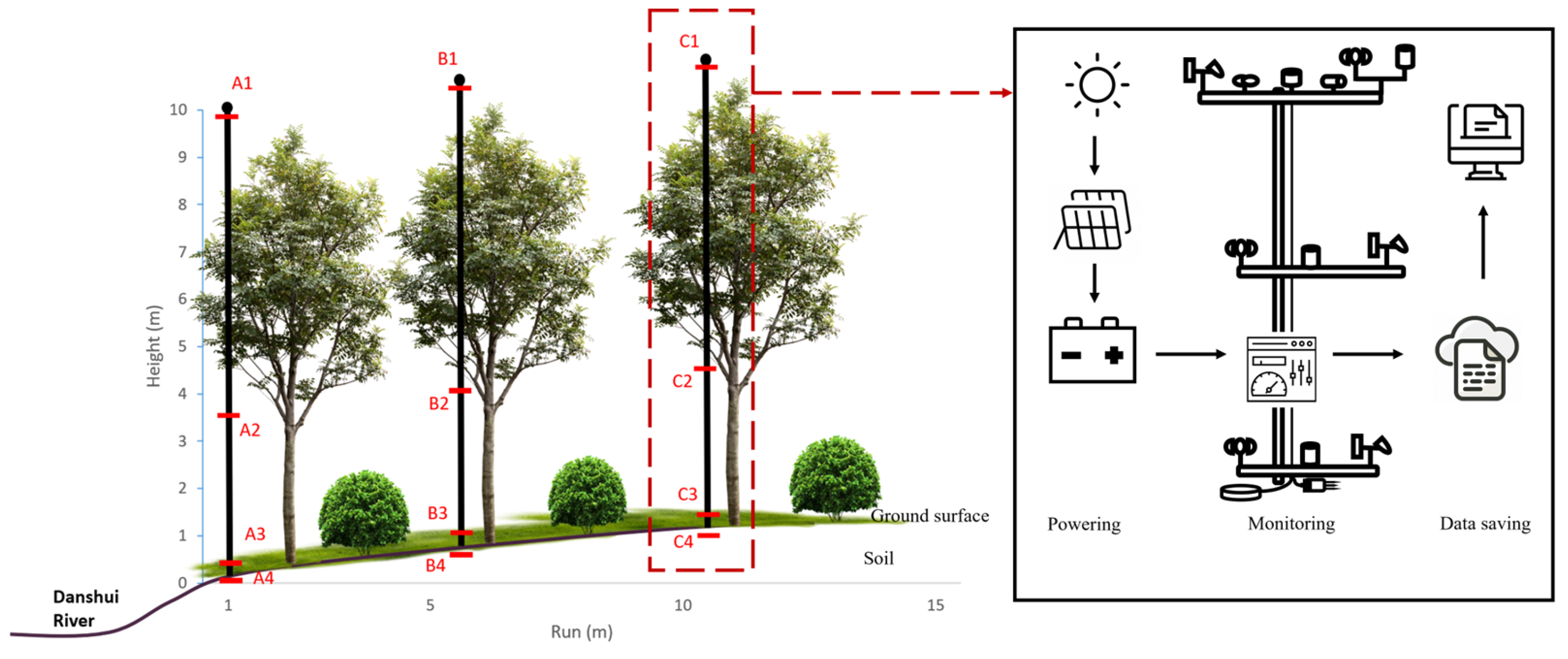
Environmental parameters are monitored at three fixed points along transects from the edge of the river—approximately 1 m, 6 m, and 11 m from the river within each site (Figure 2). Vertically, meteorological instruments are set above-canopy (10 m for broadleaf woodlands and grassland, 12 m for coniferous woodlands), below-canopy (approximately 4 m), and above-ground (0.5 m), respectively. Although a few Metasequoia glyptostroboides Hu and W. C. Cheng individuals along the river edge exceeded 15 m, the instrumented plots were established within patches where the tallest crowns were ≤12 m. Masts were therefore located so that all above-canopy sensors were at least 0.5 m higher than the nearest tree tops, ensuring unobstructed radiation measurements. Above-canopy net radiation (Rn) was measured concurrently with the soil-heat-flux campaign described in the previous study [27].
Soil temperature and soil water content are monitored at a depth of 0.03 m below ground. All instruments were pre-calibrated and checked by the manufacturers. Parameters of all sensors are listed in Table 2. Data were transmitted through a wireless network and recorded at 10-min intervals. Besides, soil characteristics (soil types and organic matter) and vegetation structure indexes, including density and tree height, are measured (Table 1).
Data were collected from 1 September 2020 to 31 August 2021. Meteorologically, the four seasons are categorized as—spring (March–May), summer (June–August), autumn (September–November), and winter (December–February). Net radiation towards the soil surface is defined as positive.

2.4. Derivation of Sensible Heat Flux (H) and Latent Heat Fluxes (LE)

Vapor pressure deficit (VPD) is the difference between the actual water vapor content in the air and the potential maximum saturated water vapor content. It reflects the temperature and humidity conditions of the atmosphere and influences the degree of stomatal closure [28]. It is calculated as follows [29]:
V P D = 0.611 e a T T + b     ( 1 R H 100 )
where V P D is vapor pressure deficit; T is the air temperature, R H is the air relative humidity; a and b are two coefficients. When T > 0, a = 17.27, b = 237.26.
The latent heat flux in forests is calculated as follows [30]:
L E = Δ R n G + ρ a C p g a V P D Δ + γ 1 + g a g c
where Δ is the slope of the saturated vapor pressure curve with respect to temperature. ρ a is air density (1.23 kg/m3), C p is 1004.67 J/kg/K, g a and g c are the aerodynamic and canopy conductance, respectively, whose calculation is referred to in previous studies [31,32,33].
The latent heat flux in grassland is calculated as follows [30]:
L E = 0.408 Δ R n G + C n γ u e s e a T + 273 Δ + γ 1 + C d u
where u is the wind speed, e s and e a are the saturated and actual vapor pressures, respectively; C n and C d are constants set for the Penman formula with hourly and daily time steps. For hourly time steps, C n is 37, and C d is 0.24 during the day and 0.96 at night. For daily time steps, C n and C d are 900 and 0.34, respectively [34]. Referring to previous studies, PAR was used to determine the daytime and nighttime. PAR ≥ 10 μmol/m2/s is defined as daytime, and PAR < 10 μmol/m2/s is defined as nighttime [32]. The daytime periods for each season are as follows: 6:00–17:00 (spring), 5:00–18:00 (summer), 6:00–16:00 (autumn), and 7:00–16:00 (winter). R n , G, T 1 , and T 2 can be directly measured by sensors to calculate the latent and sensible heat fluxes.
The same Rn dataset from the previous study was used here to force energy-balance calculations for H and LE [27].

2.5. Statistical Analysis

Differences in heat fluxes among riparian plant communities and across river-to-land distances were examined with repeated-measures Analysis of variance (ANOVA), followed by Least Significant Difference (LSD) post-hoc pairwise comparisons. Prior to analysis, the Kolmogorov–Smirnov test confirmed normality for all variables. Because net radiation is concentrated during the daytime and exhibits pronounced diurnal variation, inter-seasonal comparisons were restricted to midday heat fluxes collected on three consecutive clear-sky days in each season. Midday was defined as 12:00–14:00 h Beijing time (UTC+8). All analyses and visualizations were performed in Origin 2022.
For each plot, the arithmetic mean of heat-flux values at the three river-to-land distances was calculated to represent the community-level flux. Significance tests addressed midday net radiation, sensible heat flux (H), latent heat flux (LE) and soil heat flux among plant communities within each season; midday fluxes among vertical layering categories (arbor–shrub–grass vs. arbor–grass) within each season; midday fluxes among functional types (evergreen broad-leaf, deciduous broad-leaf, coniferous) within each season; and seasonal variation in midday fluxes within each community.
Significance tests for river-to-land distance effects were applied to midday H, LE, and soil heat flux only. Analyses encompassed differences among distances within a single community and season, differences among distances within each functional type and season, differences among distances within each vertical layering class and season, and seasonal contrasts of distance effects within each community.

2.6. Data Quality Control and Analysis

Prior to statistical analysis, quality assurance procedures encompassing outlier screening (de-spiking) and missing-data interpolation (gap-filling) were implemented [35]. The de-spiking protocol involved visualizing time-series data to verify adherence to characteristic diurnal and seasonal cycles, thereby identifying residual anomalies indicative of intermittent instrument malfunctions. Table A2 in Appendix A summarizes the proportions of missing values and excluded outliers relative to the total samples for each parameter across research sites. Single ten-minute gaps were imputed using the mean of observations from two adjacent time intervals. For consecutive gaps, daytime and nighttime data were replaced by averaging values within 14-day and 7-day time windows, respectively, centered on the same timestamp [36].
For the daily scale analysis, all data are compiled into hourly averages, and three consecutive sunny days (defined as three days before which no rain is found) in each season are chosen. 14th–16th April (2021), 11th–13th July (2021), 28th–30th October (2020), and 6th–8th February (2021) represent spring, summer, autumn, and winter, respectively. For the annual scale analysis, the data are compiled into 24-h averages. For temporal variations of heat fluxes, all environmental parameters monitored within each riparian plant community are averaged to represent the whole research site. For spatial distributions of heat fluxes, environmental parameters (above-canopy, under-canopy, and above-ground) monitored at the same distance from the river within each plant community are averaged.
Interpretable Machine Learning (IML) is applied to explore the relative importance, non-linear relationships, and interactions of parameters of meteorology, soil, vegetation, and the river to H and LE on both daily and annual temporal scales. Since variables include continuous and categorical ones, five commonly used machine learning models were chosen based on model fitting performance and stability: LightGBM (Lightweight Gradient Boosting Machine), Support Vector Regression (SVR), Multi-Layer Perceptron Regression (MLP Regression), Random Forest Regressor, and Extreme Gradient Boosting (XGBoost). For the five machine learning algorithms employed in this study, automated hyperparameter optimization was implemented using the Tree-structured Parzen Estimator (TPE) algorithm within the Optuna framework. This approach leverages Bayesian probabilistic modeling to iteratively refine hyperparameter configurations, maximizing objective metrics while minimizing computational resource expenditure [37]; 80% of the dataset was used as the training set, and 20% as the validation set. R2 (coefficient of determination), RMSE (root mean square error), and MAE (mean absolute error) are chosen as the evaluation metrics for model performance. After determining the model with the best overall performance, we utilized SHAP (SHapley Additive Explanations) to interpret the regression model outputs. The related analyses are completed on the Python 3.13 platform.
For riparian grassland, eight parameters concluding soil temperature (Ts), soil water content (SWC), vapor pressure deficit (VPD), wind speed (u), net radiation (Rn), photosynthetically active radiation (PAR), sunshine duration (SUN) and distance are chosen and for riparian forests, sixteen parameters concluding tree height (TH), canopy height (CH), canopy width (CW), LAI, canopy closure (CC), canopy porosity (CP), vertical layering (VL), soil organic matter (SOM), Ts, SWC, VPD, u, Rn, PAR, SUN and distance are chosen.

3. Results

3.1. Temporal Variations of Environmental Parameters

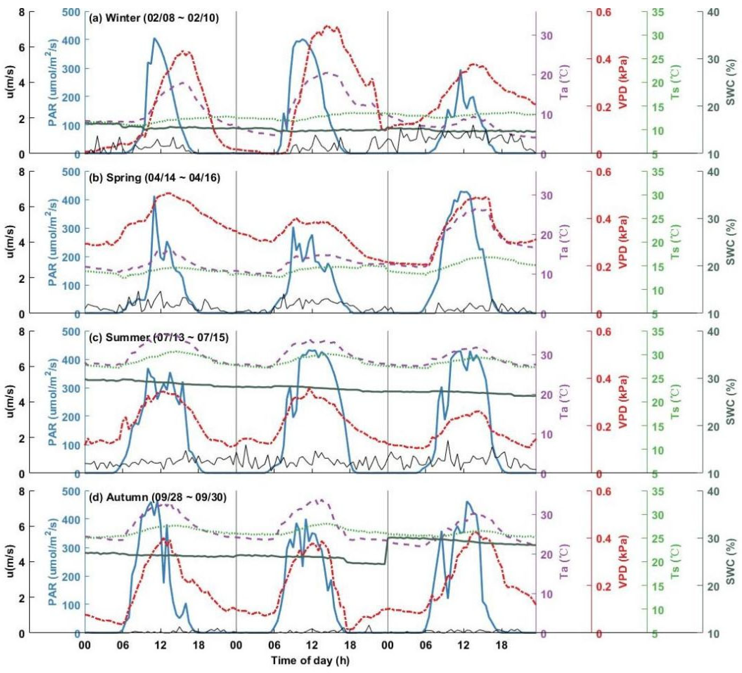
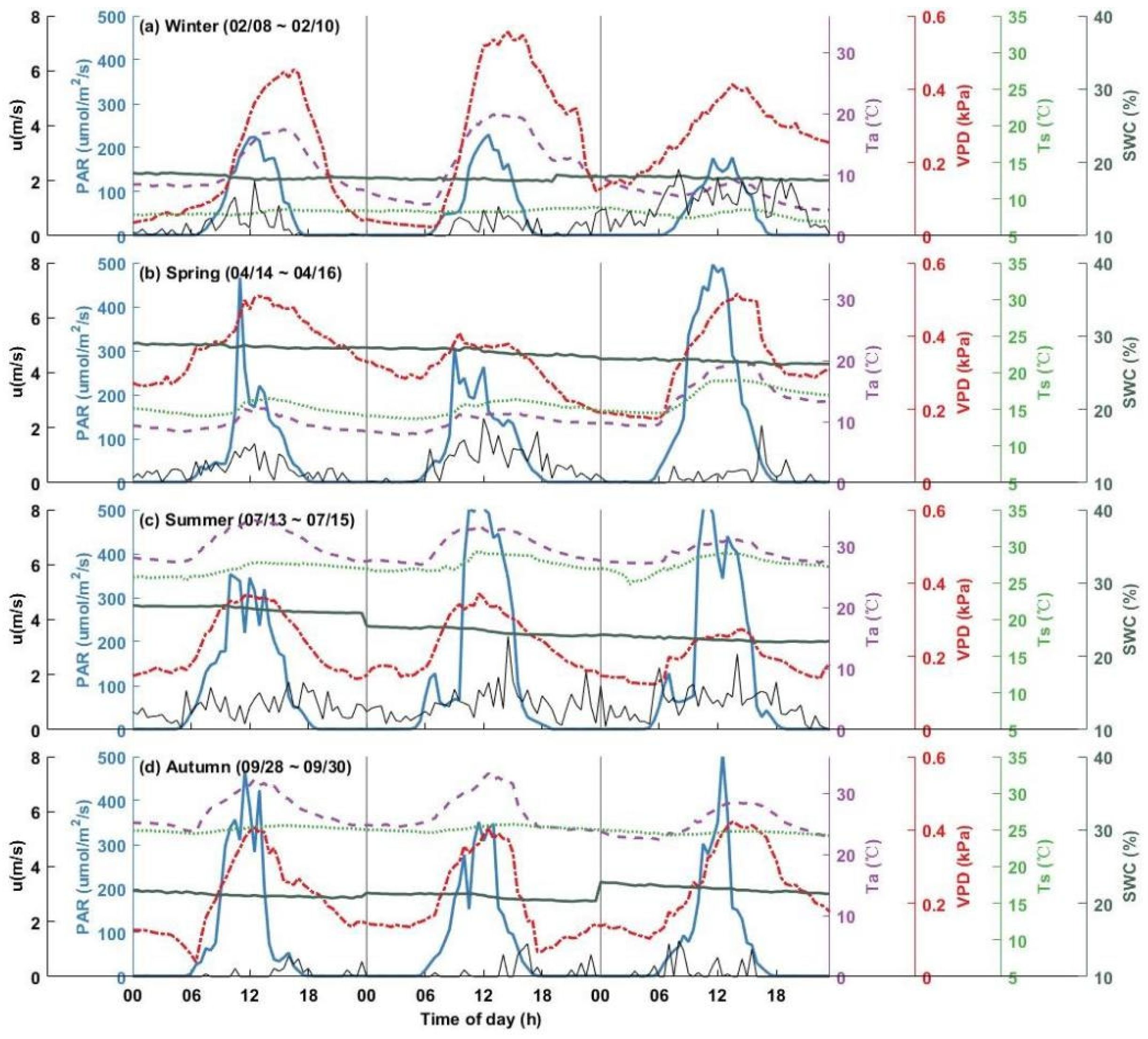
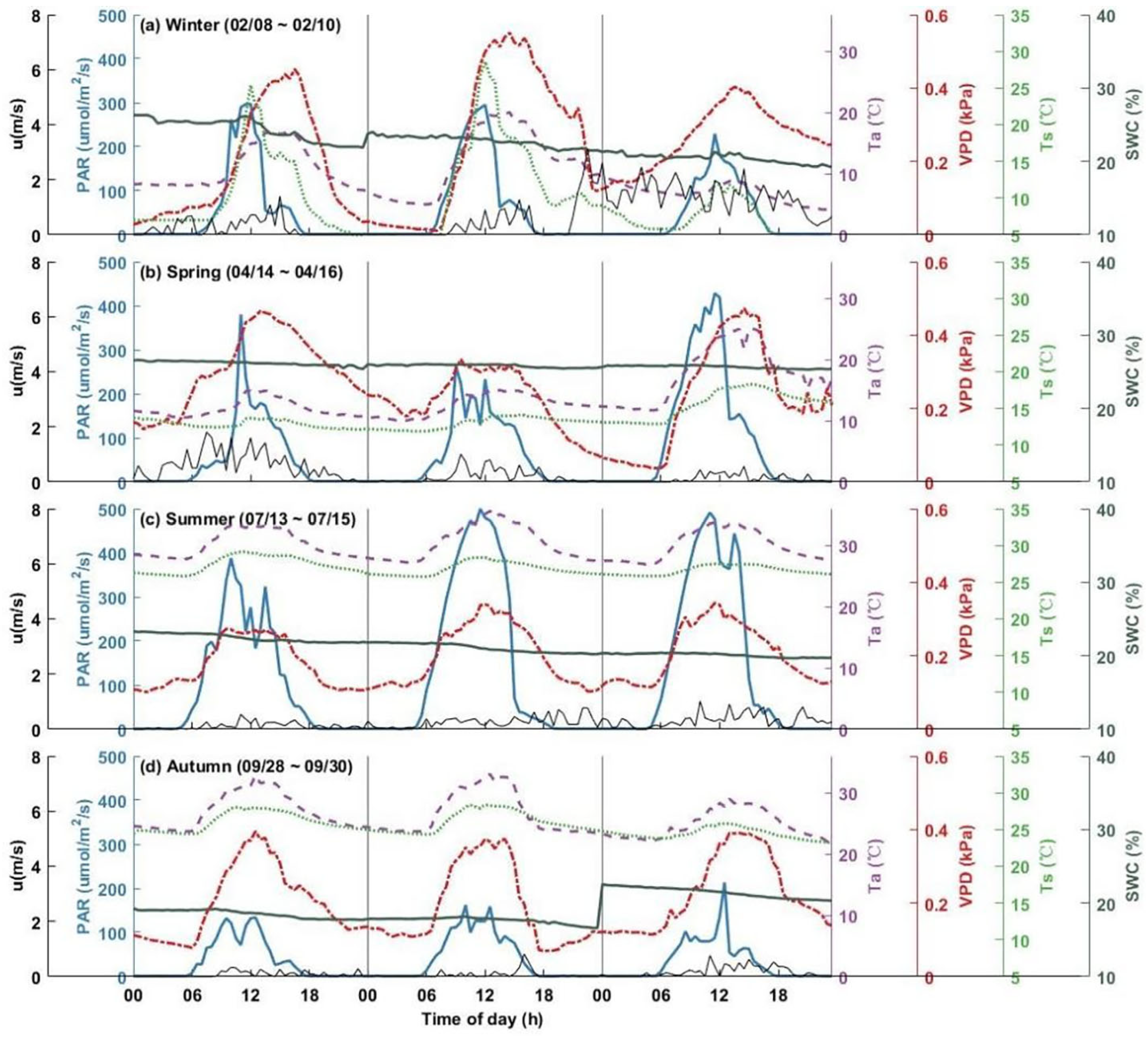
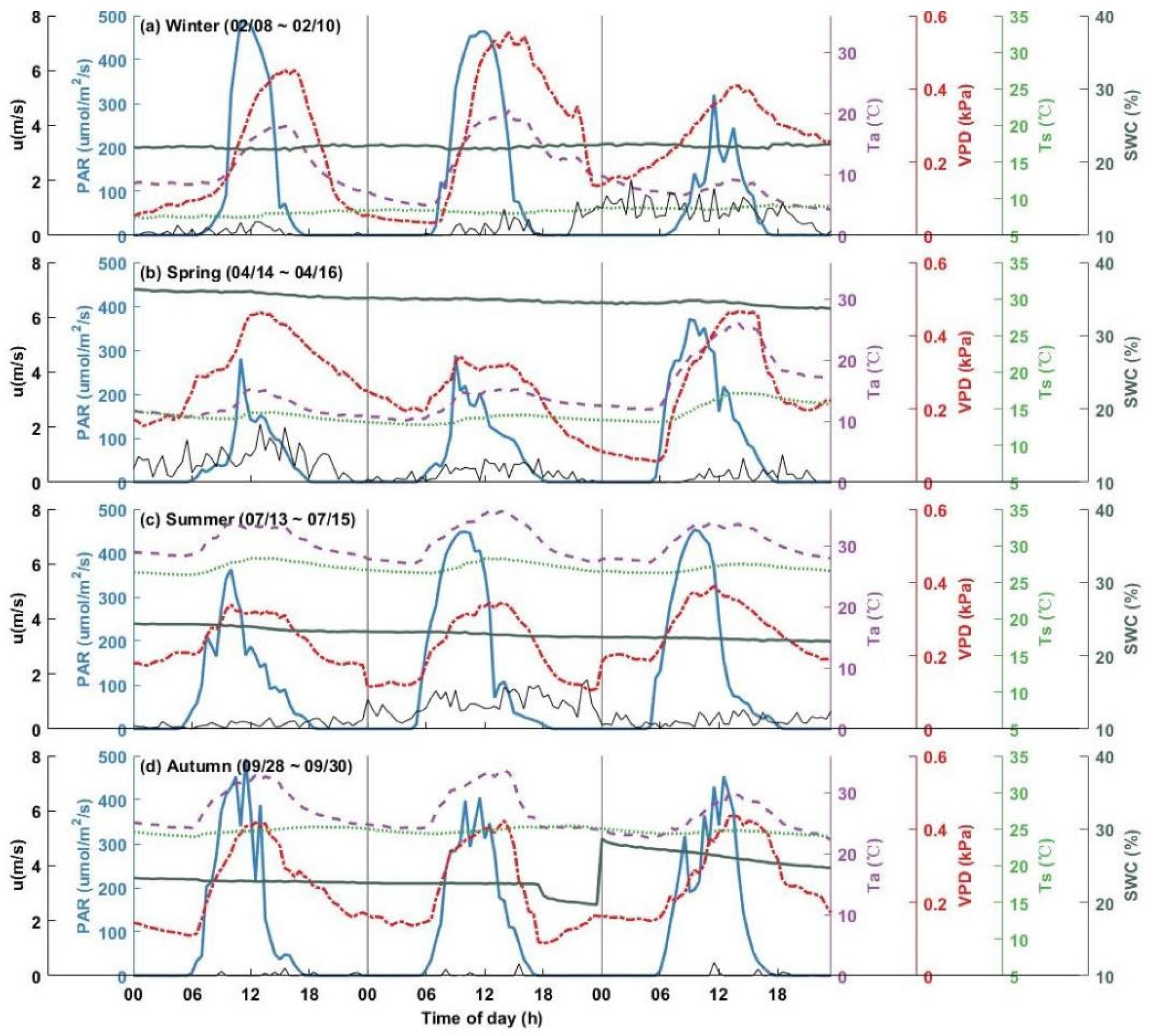
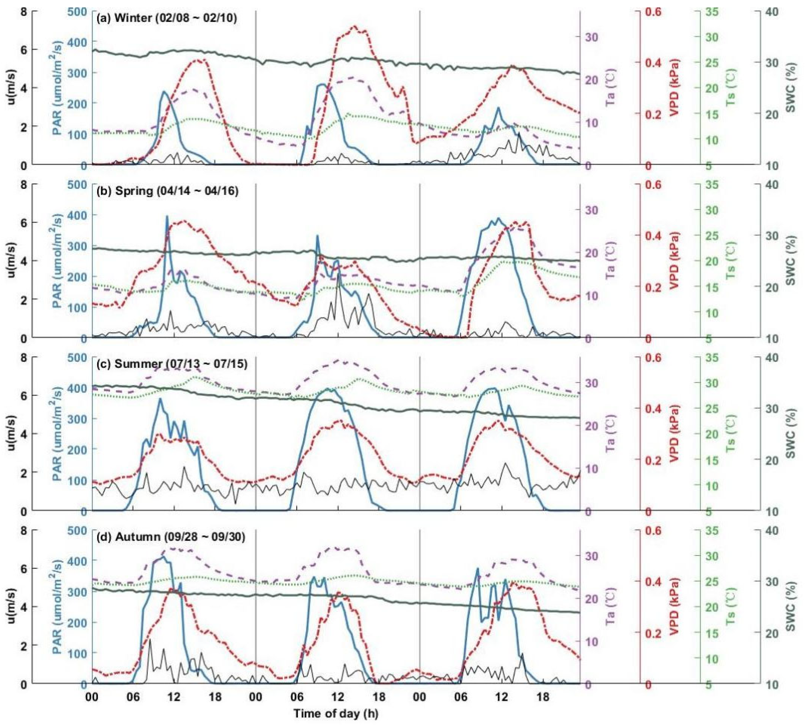
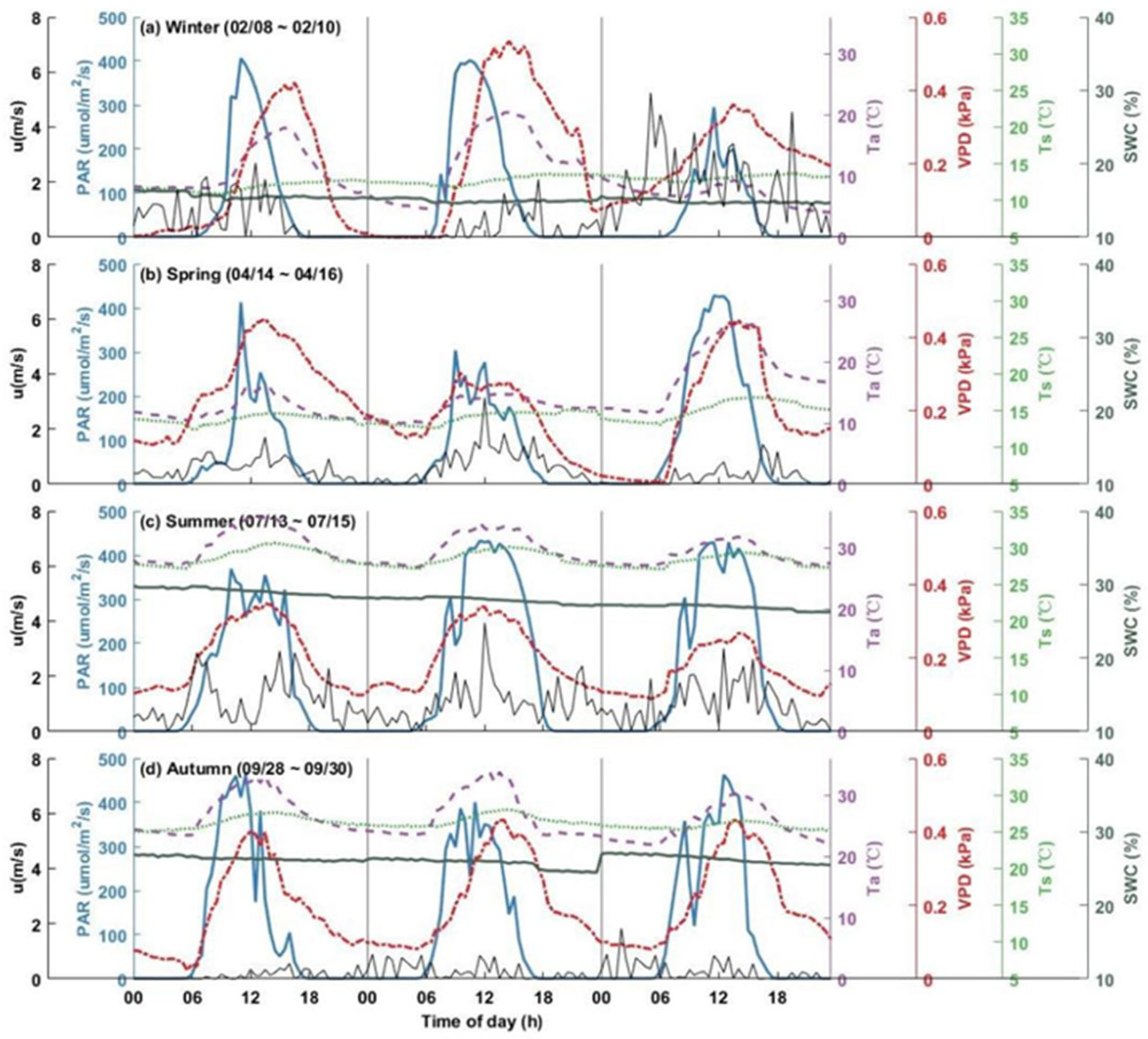
Since environmental parameters in each riparian site show similar diurnal trends on sunny days, only CH is selected and shown in Figure 3. Diurnal trends in other research sites are seen in Appendix A (Figure A1, Figure A2, Figure A3, Figure A4, Figure A5 and Figure A6). PAR rose fast in the morning. It peaked at midday at 287.9–451.7 μmol/m2/s. It fell slowly at night. Ta and VPD went up and then down. Summer Ta was 27.1–36.1 °C. Winter Ta was 3.95–9.5 °C. Winter VPD max was 0.53 kPa. Summer VPD max was 0.26 kPa. Ts made a small sine curve. SWC went down, up, then down again. It stayed between 18.8% and 35.1%. Sunshine lasted 10, 12, 14, and 11 h each season. Wind speed in the grassland fluctuated during the day, with a maximum value of 5.25 m/s.
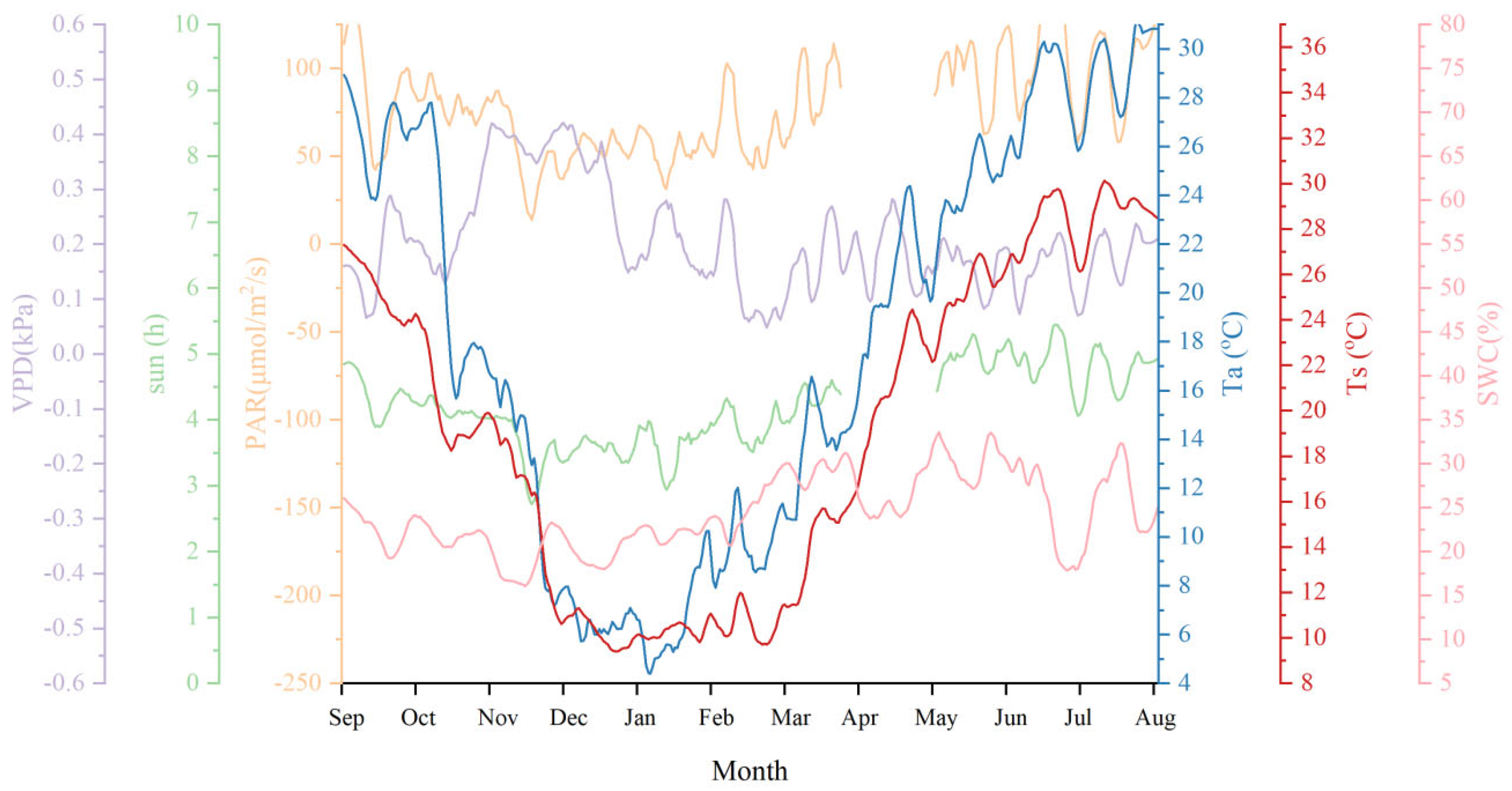
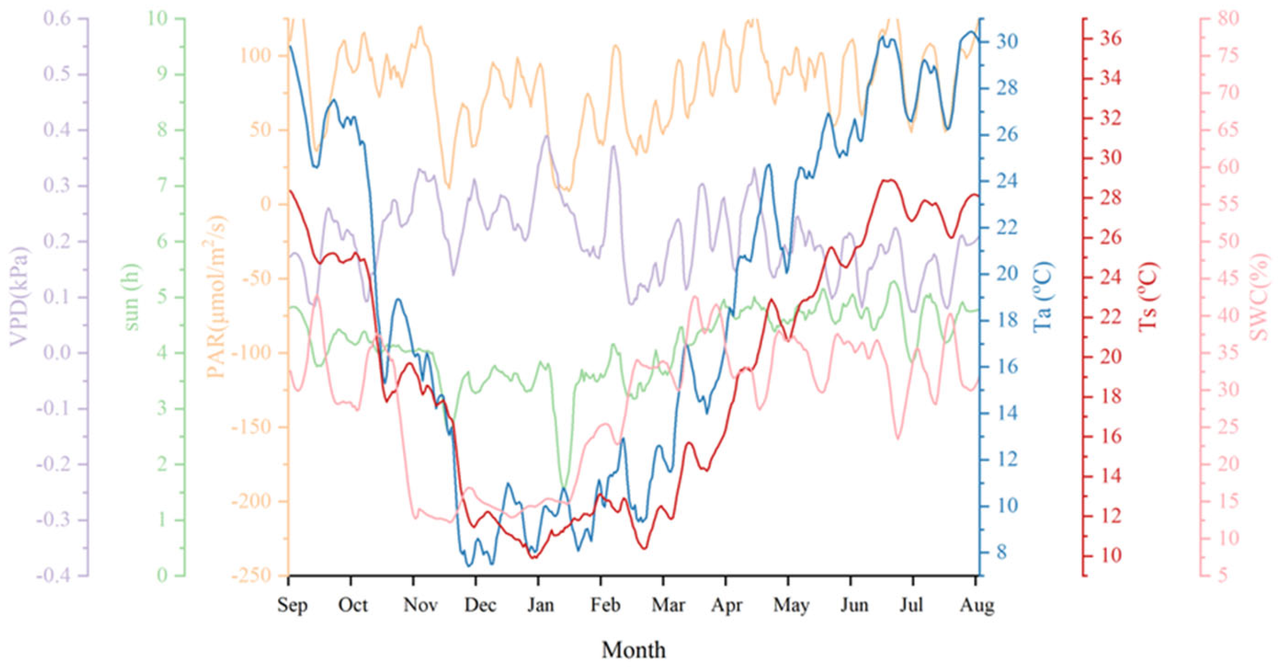
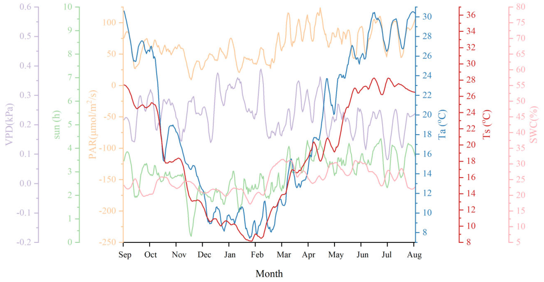
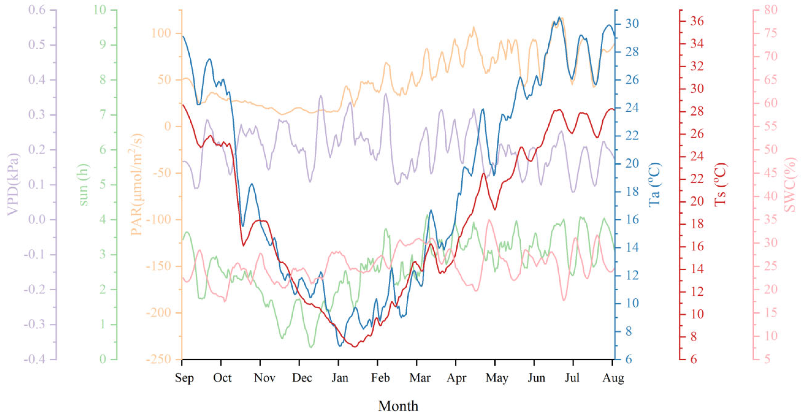
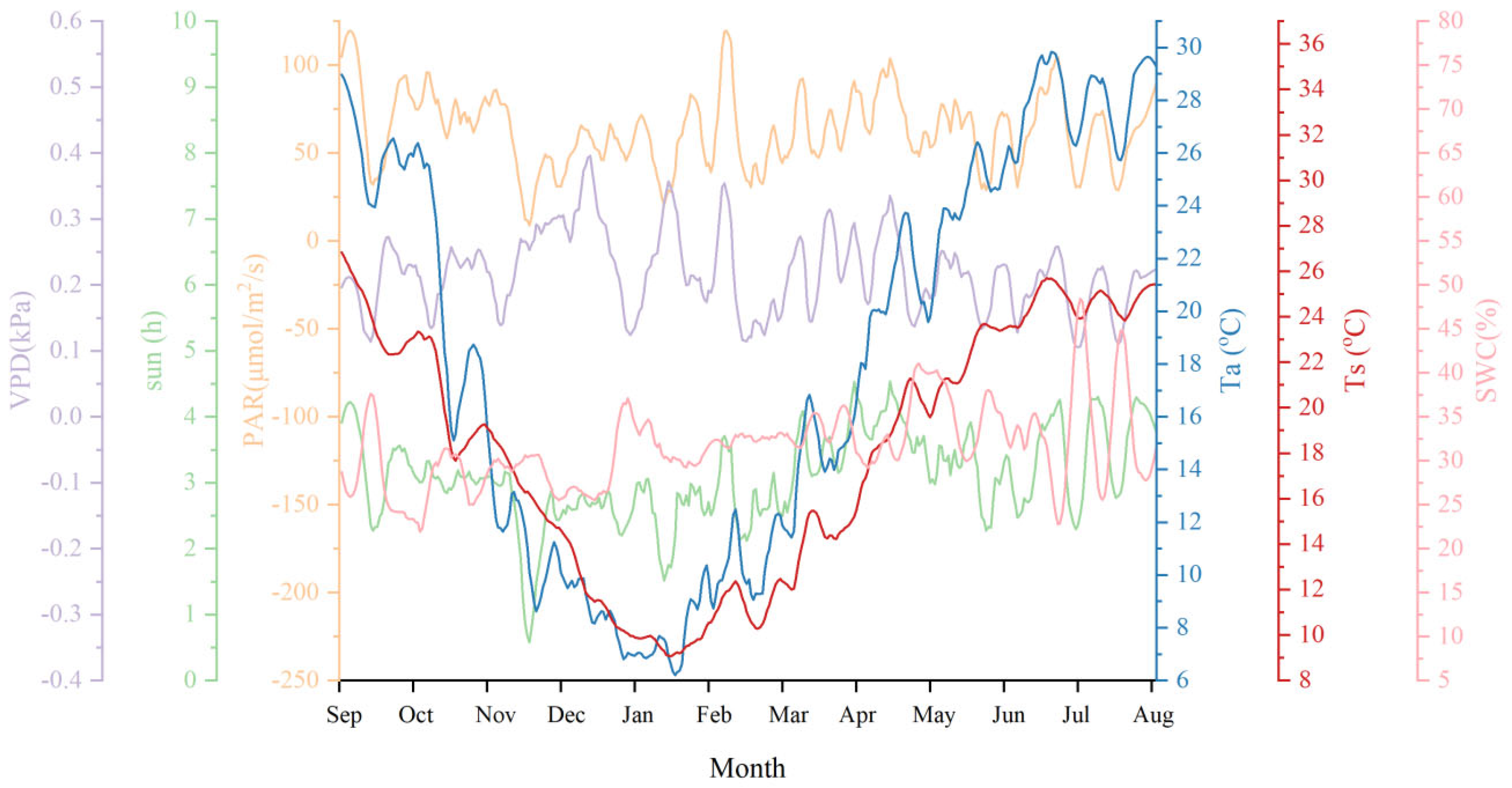
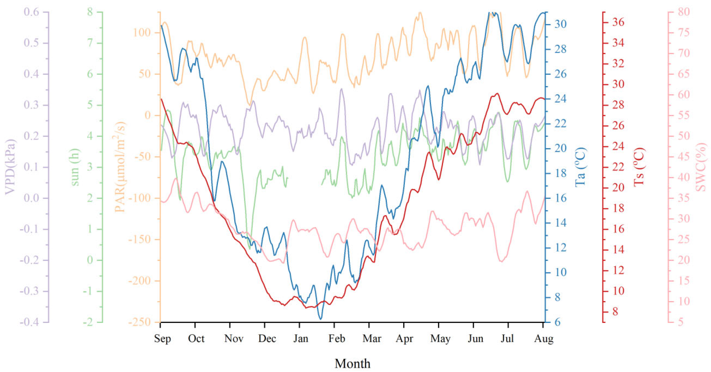
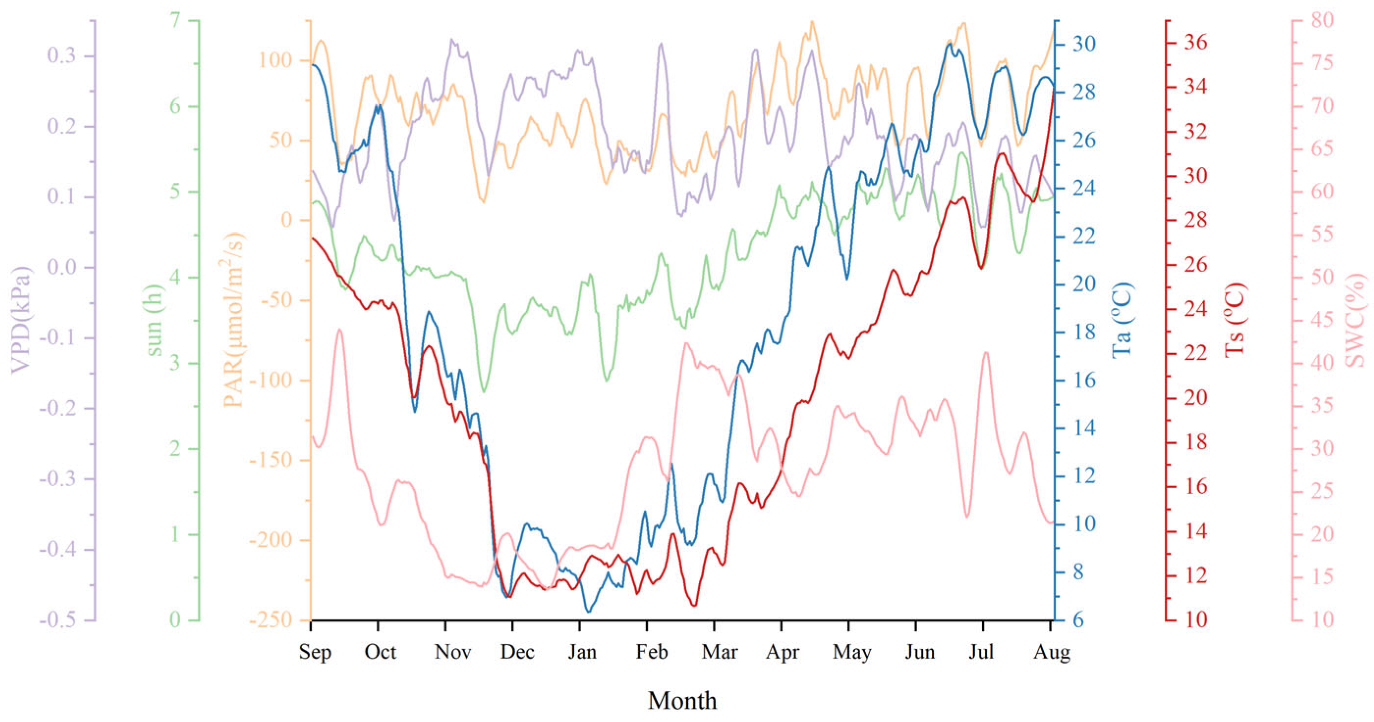
Season trends were the same. Figure 4 shows CCO. The rest in other sites are listed in Appendix A (Figure A7, Figure A8, Figure A9, Figure A10, Figure A11 and Figure A12). Ta and Ts were lowest in winter and highest in summer. Ta max was 31.92–33.47 °C. Ta min was 1.96–5.31 °C. Ts changed less. PAR was always positive. Its max was 136.66–166.33 μmol/m2/s. VPD was 0–0.52 kPa. SWC was 11.80%–51.38%.

3.2. Spatial Distribution of Environmental Parameters

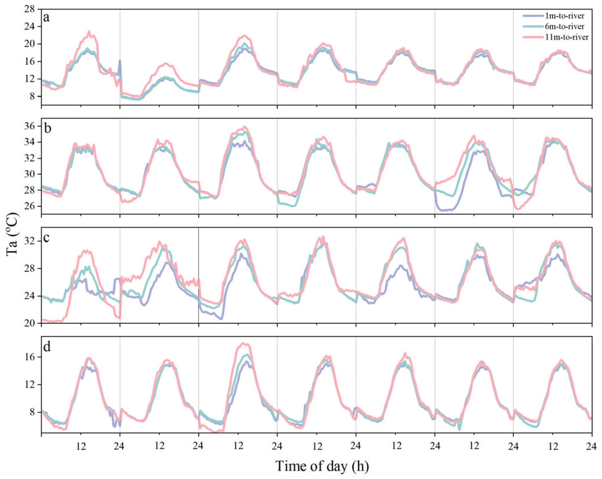
Tempo-spatial distributions of each environmental parameter in the site of CCO on the daily scale are shown in Figure 5, Figure 6, Figure 7, Figure 8, Figure 9 and Figure 10. During the daytime, as the distance from the river increases (Figure 5), the Ta value continuously rises, confirming the cooling effect of the water body [31]. The rise is strongest at midday, when evaporation is high. Shi et al. [38] measured +0.38 °C per 1 m from the river in the lawn. Cooling is weaker in winter than in summer [39].
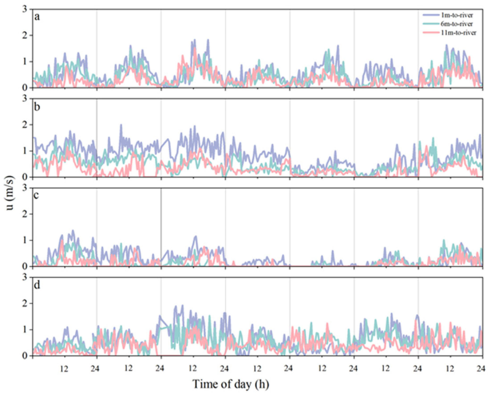
Wind speed at each riparian site keeps changing (Figure 6). Day values are higher than night values. Average wind speed drops as the distance from the river grows, so the water body raises the wind speed. In the same season, every point in CH is windier than in the forest. Tall forests with high LAI, like conifer-shrub-grass, show lower and steadier wind speed.
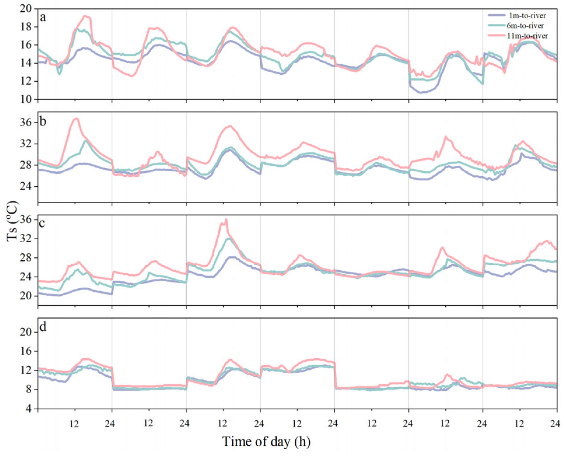
The influence of distance from the river on Ts is mainly reflected in its peak values and diurnal variation patterns (Figure 7). During the daytime, across all four seasons, the peak values increase with greater distance from the river. At night, the effect of increasing distance from the river on soil temperature can be categorized into two patterns: in summer, Ts in all communities increase with distance from the river during nighttime; conversely, in spring, the site of CMO shows the opposite trend.
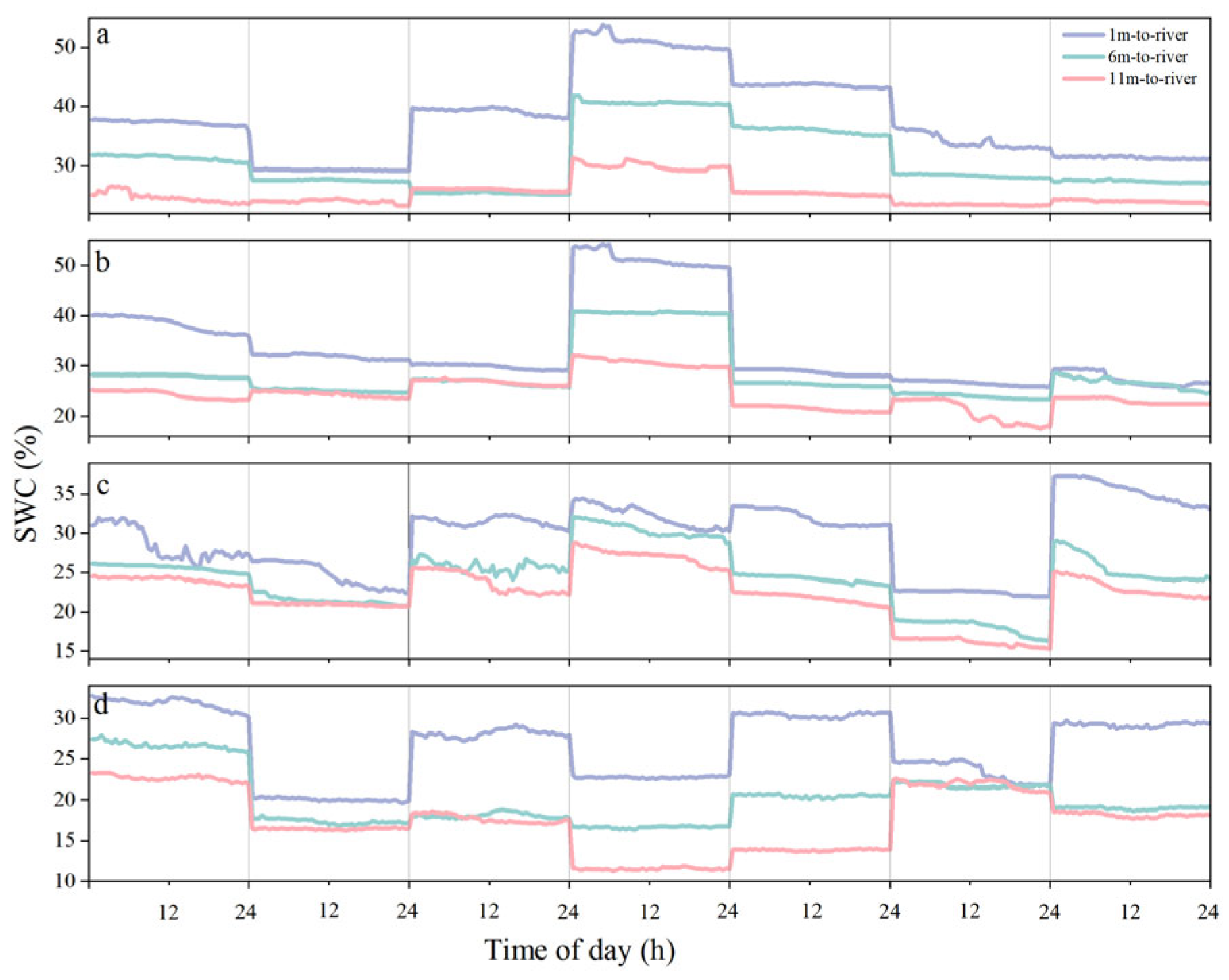
In all riparian zones, the daily variation in SWC was generally stable, with soil moisture decreasing as the distance from the river increased (Figure 8). Seasonally, it is highest in spring and summer, followed by autumn and winter. The maximum and minimum values are both observed in the CCH. The influence of the river on soil moisture was more pronounced in grasslands and broadleaf forests, but less evident in the conifers. In CH, SWC at 6 m and 11 m from the river is significantly lower than at 1 m, while the difference between the 6-m and 11-m points is relatively small across all seasons, indicating that the river’s influence on SWC weakens with increasing distance.
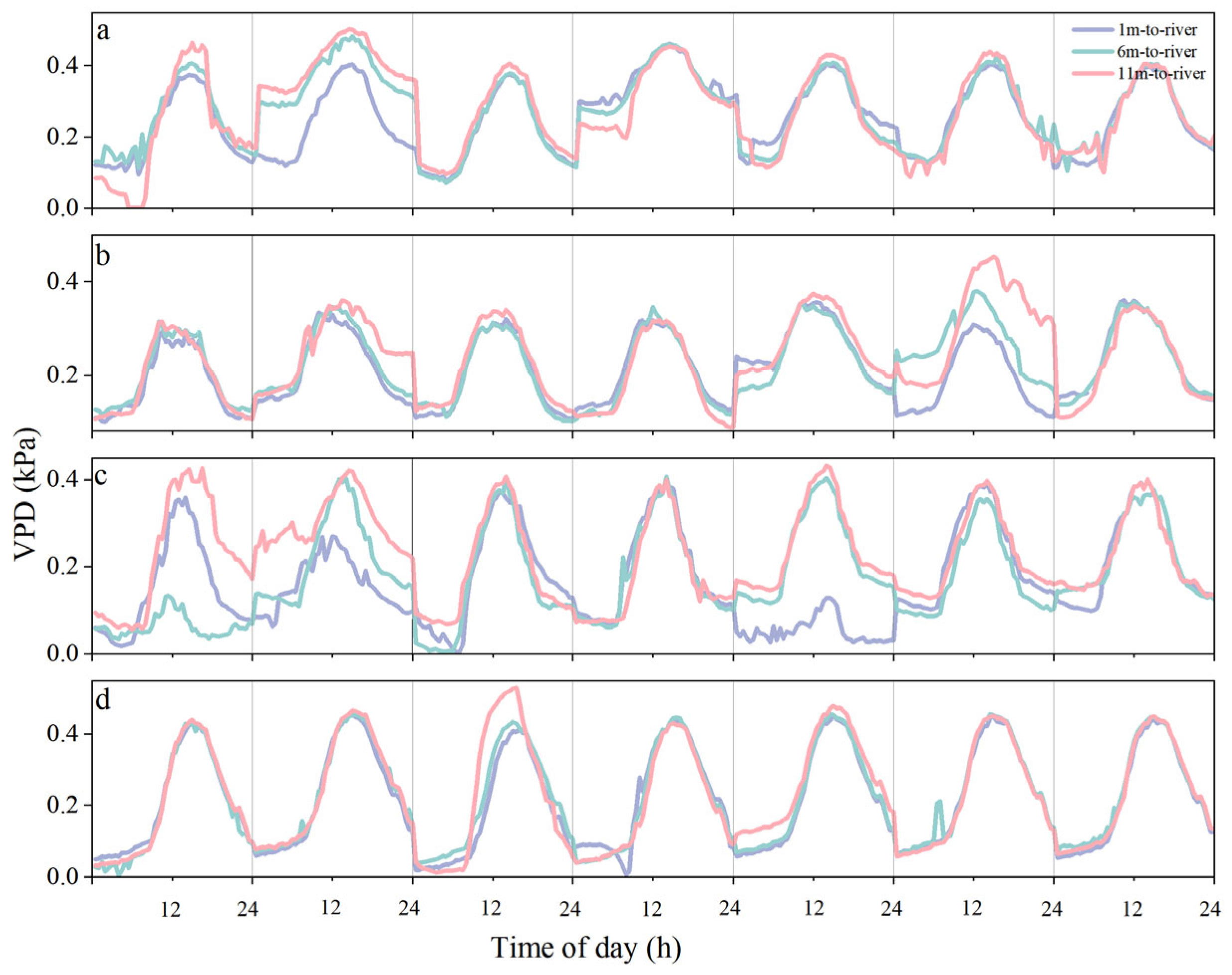
VPD rose with distance from the river in all seasons (Figure 9), so values were lowest near the water. Peak VPD differed by community. In summer, the daily VPD range grew with distance; in winter, it shrank. CH had lower VPD than forests; conifers had the highest. These differences among community types are mainly due to variations in the sources of atmospheric moisture within the plant communities, which primarily come from soil evaporation and vegetation transpiration [40]. Trees, shrubs, and grasses differ in their transpiration capacity, with trees generally having higher transpiration rates and grasses having lower.
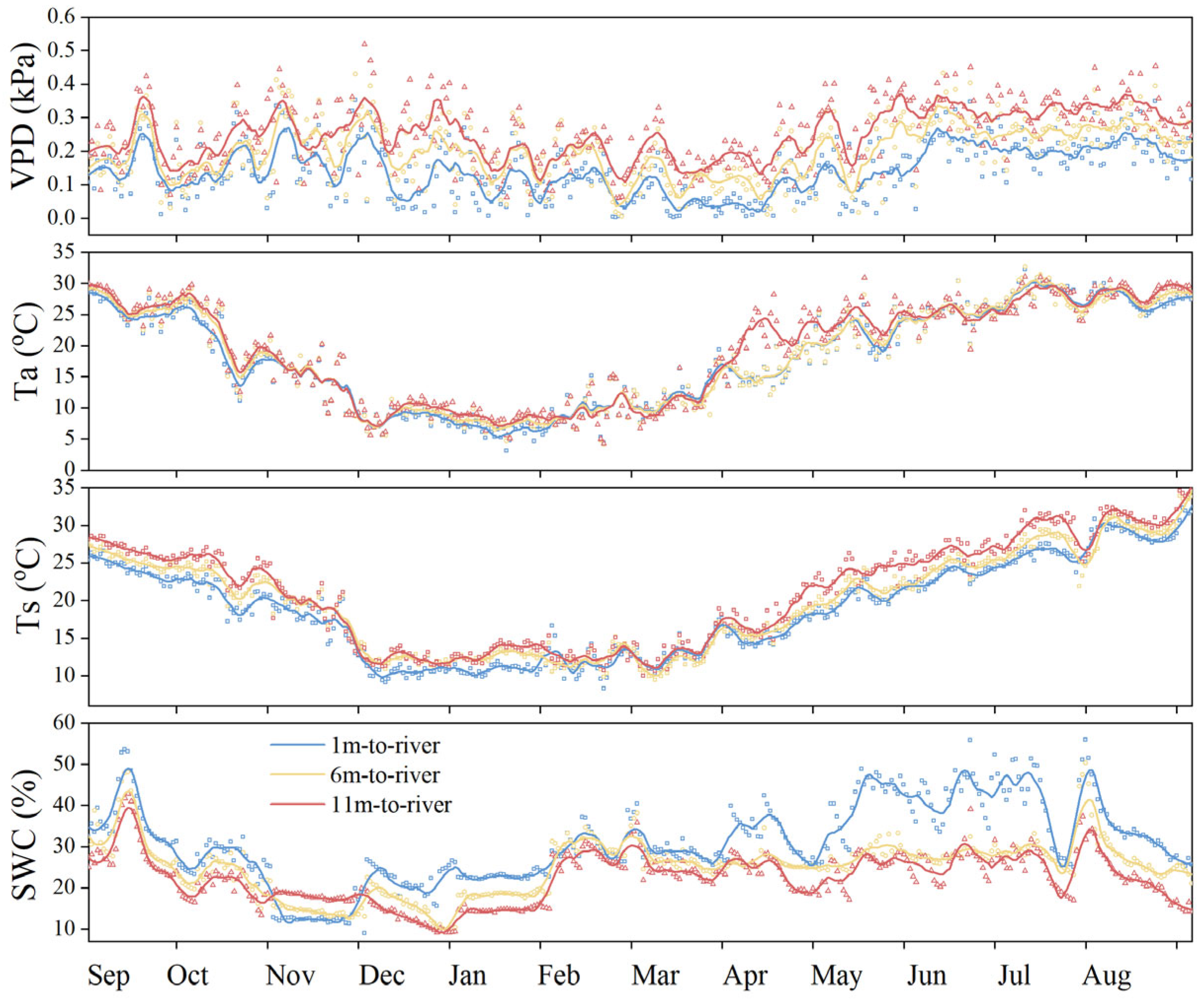
Daily Ta is lower near the river at every site (Figure 10), so the water cools the Shanghai riparian zone all year, most in summer. Distance effect on Ta differs among plant types, showing joint cooling by water and plants.
Ts increases with distance from the river in CH. The river’s influence is most pronounced in summer, where water-mediated cooling shows a greater effect on Ts than Ta. In winter, Ts shows minimal variation across distances. From spring to autumn, broadleaf sites far from the river have higher Ts.
SWC is always highest at 1 m and lowest at 11 m in every season. VPD fluctuates annually at different distances but generally follows the pattern: highest at 1 m and lowest at 11 m.

3.3. Temporal Variations of H and LE

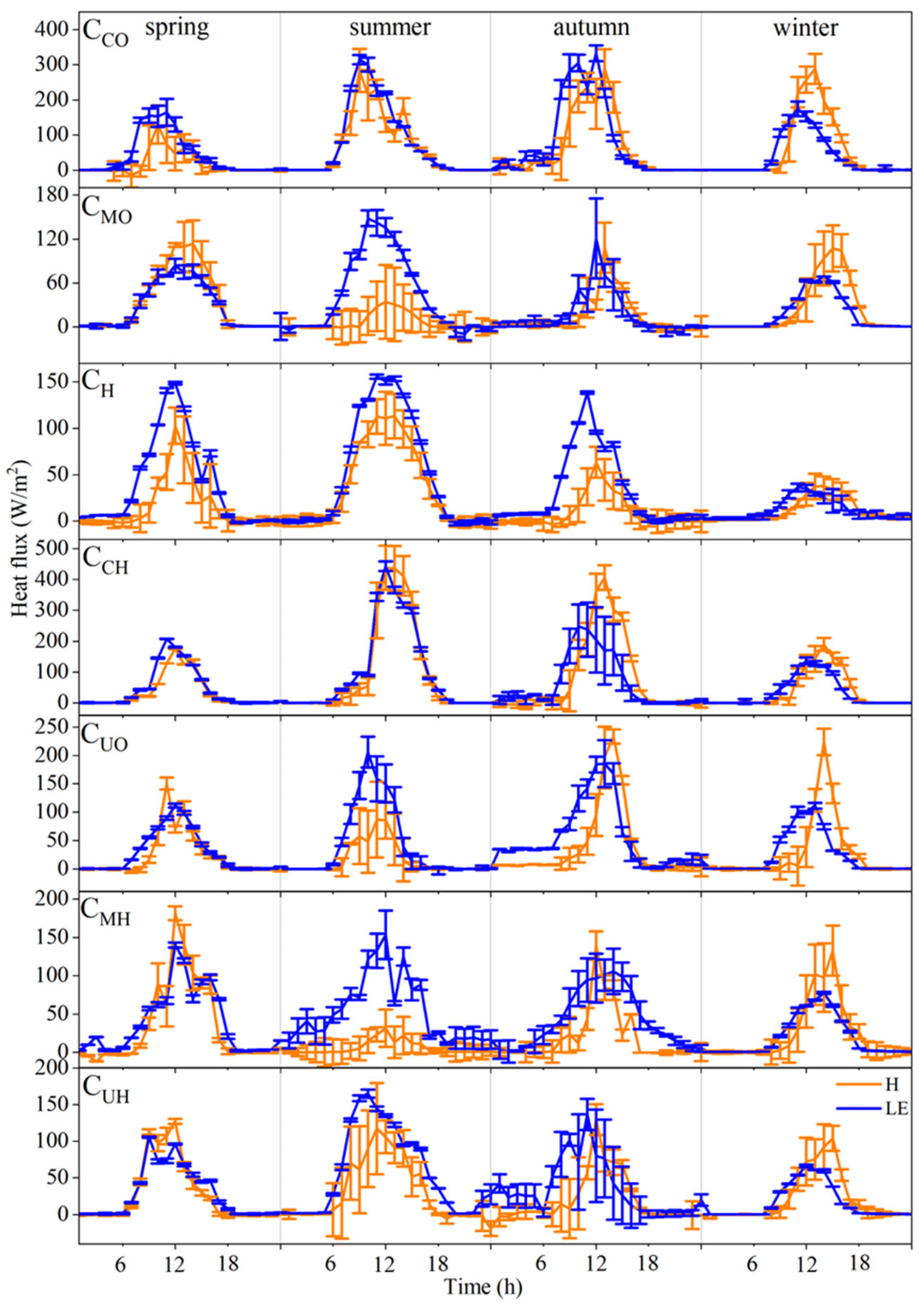
Sensible heat flux exhibited a unimodal diurnal pattern (Figure 11) generally synchronized with net radiation, whose diurnal variation is not shown here. Its magnitude is primarily governed by atmospheric turbulent motion [41]. During midday, enhanced canopy-level turbulent exchange due to elevated temperatures and wind speeds drives H to peak values, though with greater variability than net radiation.
Previous energy exchange studies have documented that wetlands with grasslands and shrubs typically demonstrate negative daytime H values [42], while an urban grassland shows positive H fluxes [43], which is consistent with our observations. Both H and LE display sinusoidal variations with pronounced phase lags over water bodies [44]. More heat storage of the water body, resulting from its high specific heat capacity, makes decoupled H/LE fluxes relative to net radiation timing [45]. On our site, H keeps a single noon peak close to net radiation, with only a small winter lag. Riparian grass H equals 102.97 W/m2 in spring, 113.28 W/m2 in summer, 63.39 W/m2 in autumn, and 37.91 W/m2 in winter. It is consistent with the daily variation range of H in Inner Mongolian grasslands and reed communities in riparian zones of semi-humid regions [46], but higher than that of the lawn in Beijing urban areas throughout the year [47]. Due to the canopy buffer on sensible heat transfer between the ground and the air, the sensible heat flux of different forested communities exhibits distinct seasonal differences during the vegetation growth process. In summer, H is greater in broad-leaved communities than in conifers and for the former ones, and higher in two-layered sites than in three-layered sites since shrubs can provide shading by filling the space between tree trunks and blocking radiation [48]. Maximum values are from 31.27 W/m2 (CMH) to 438.07 W/m2 (CCH).
In summer, LE swings more than H each day; in winter, H swings more, as seen in Poyang Lake floods [45]. Daily LE in every riparian site shows either one peak or two peaks (e.g., CMH in summer). The two-peak type rises, drops at noon, then rises again; this “midday depression of transpiration” [49] appears in summer and autumn when high temperature closes stomata and plants cut water loss [46]. The same pattern is reported for urban green space [50]. CCH gains the most latent heat, peaking at 443.10 W/m2 in summer; CH gains the least, peaking at 36.10 W/m2 in winter.
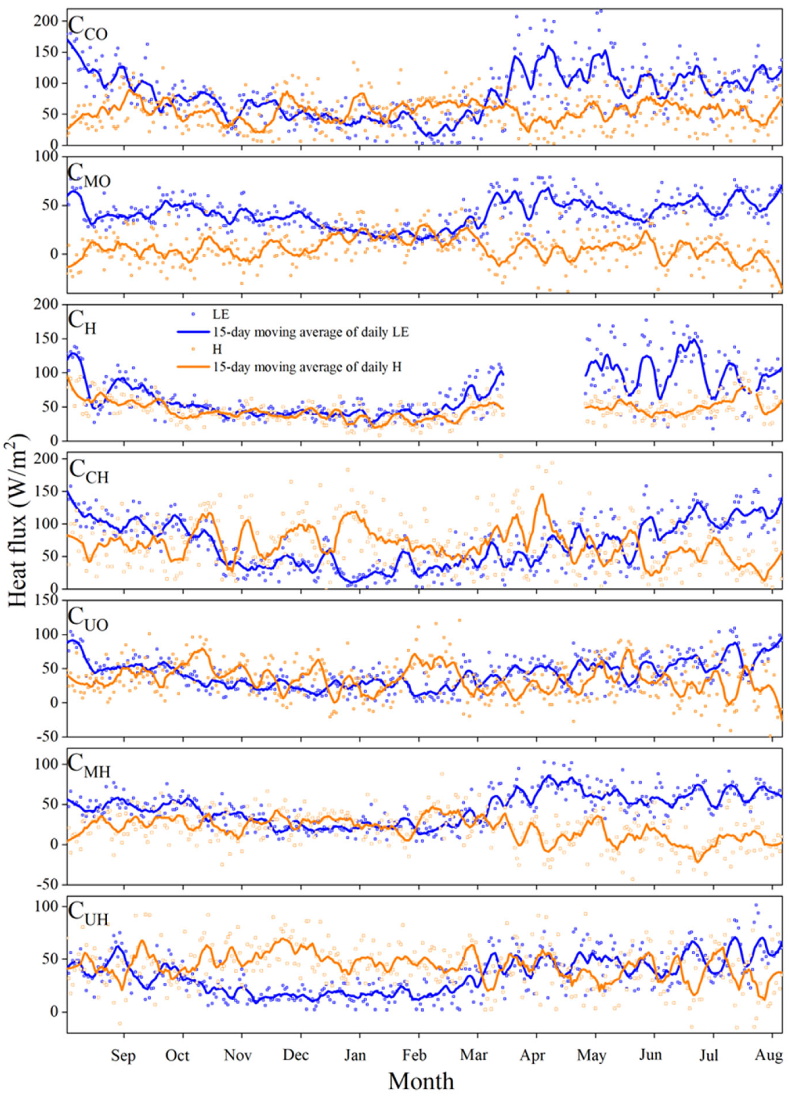
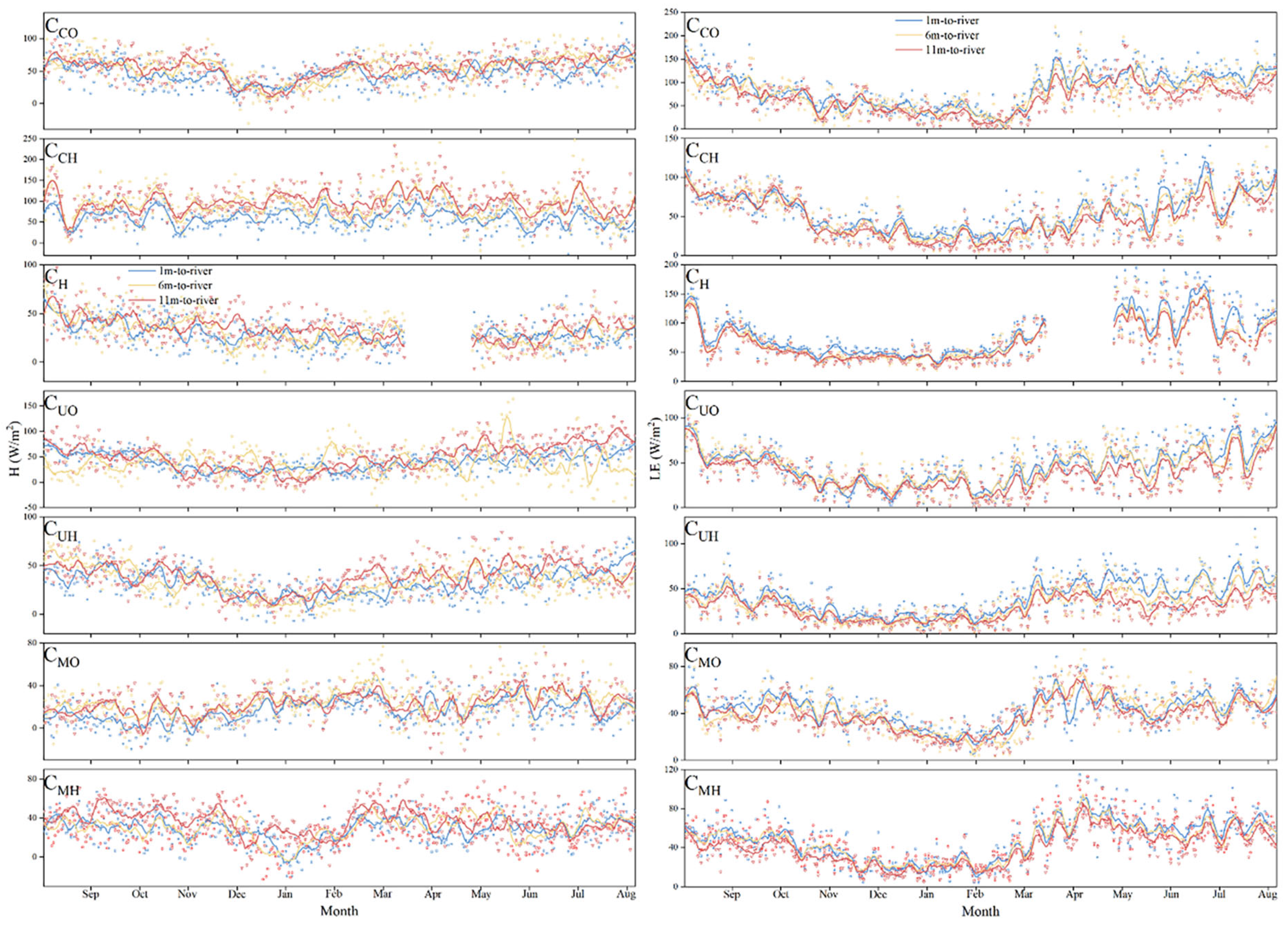
Seasonal variations of daily averaged H and LE exhibit as higher in spring and summer, lower in autumn and winter. H in all plant communities is constantly positive (Figure 12). LE in grassland and evergreen broadleaved sites remains positive, but negative in conifers and deciduous broadleaved sites during summer, indicating that conifers and deciduous broadleaved forests exert a stronger microclimate regulation effect, showing as cooling in summer and heating in winter. Daily-averaged LEmax ranges from 78.73 W/m2 (CMO) to 216.01 W/m2 (CCO). At the same time, Hmax ranges from −48.75 W/m2 (CUH) to 231.14 W/m2 (CCH). Energy exchange within different climatic zones and different ecosystems varies significantly. Yuan et al. [51] found that the seasonal variation of H in riparian shrubs in semiarid areas is opposite to that of LE. The seasonal variation trend of H in the Beijing urban green space ecosystem, however, shows no obvious pattern [52].

3.4. Spatial Distributions of H and LE

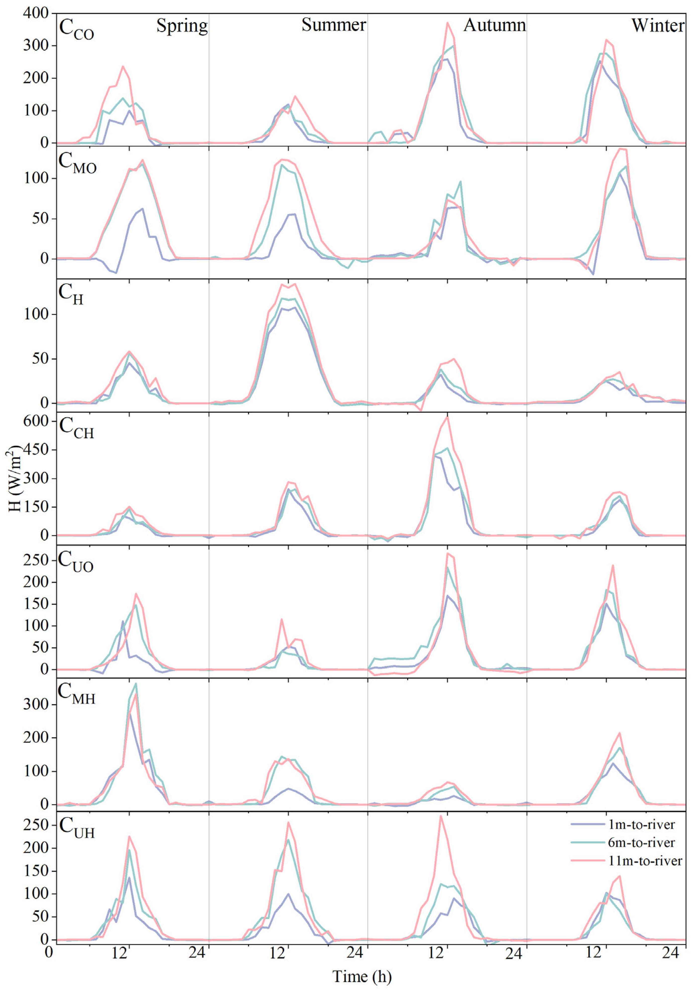
Due to the horizontal air flow between the river and land forming a secondary wind field [53], sensible heat flux gradients occur within riparian grasslands and broad-leaved sites in spring, summer, and autumn (Figure 13). These gradients are mostly larger farther from the river and smaller closer to the river, which reflects the mitigating effect of water bodies on sensible heat exchange in riparian areas. Similarly, non-linear gradients in microclimate parameters (e.g., air temperature and soil temperature) have been reported in previous riparian studies [54,55]. In coniferous communities, the sensible heat flux gradient is not obvious in all four seasons. This indicates that the coniferous canopy weakens the effect of water bodies on the sensible heat flux gradient.
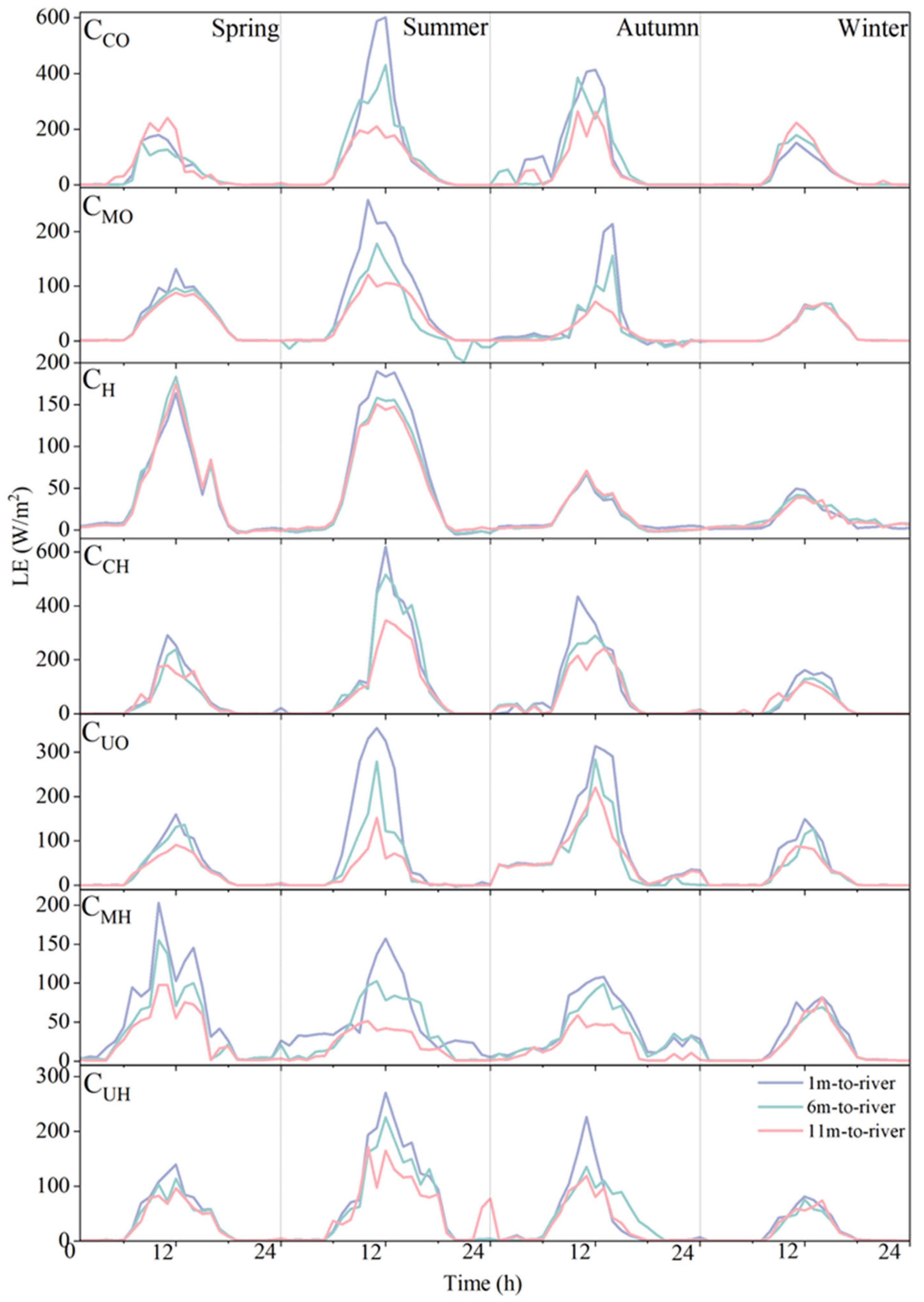
Gradients of LE in riparian areas are the opposite of H (Figure 14). Its value decreases with increasing distance from the river in spring, summer, and autumn. Meanwhile, as the distance from the river increases, the latent heat consumption shifts from water evaporation to vegetation transpiration. This causes the daily variation pattern of LE in some plant communities to change from “single—peaked” to “double—peaked” (such as in CCO and CCH).
Water bodies create certain heat flux gradients within communities, which are influenced by vegetation. In riparian grasslands and broad-leaved sites, both the daily mean H and LE show distinct gradient effects (Figure 15). The sensible heat flux values are generally higher and more variable farther from the river, and lower and more stable closer to the river. The latent heat flux values mostly peak at 1 m and are smallest at 11 m. Due to the path of bare soil in CCO, no LE gradients are observed, indicating that the effect of canopies is larger than the river on riparian energy exchange. Also, Rambo and Malcolm [56] propose that canopy gaps can offset the microclimate-regulating effects of rivers. The gradients within the community are mostly concentrated in spring and summer. Coniferous communities weaken the heat flux gradient effect created by water bodies, making the gradients of sensible and latent heat flux within them not obvious.

3.5. Machine-Learning-Based Attribution of Heat-Flux Variability

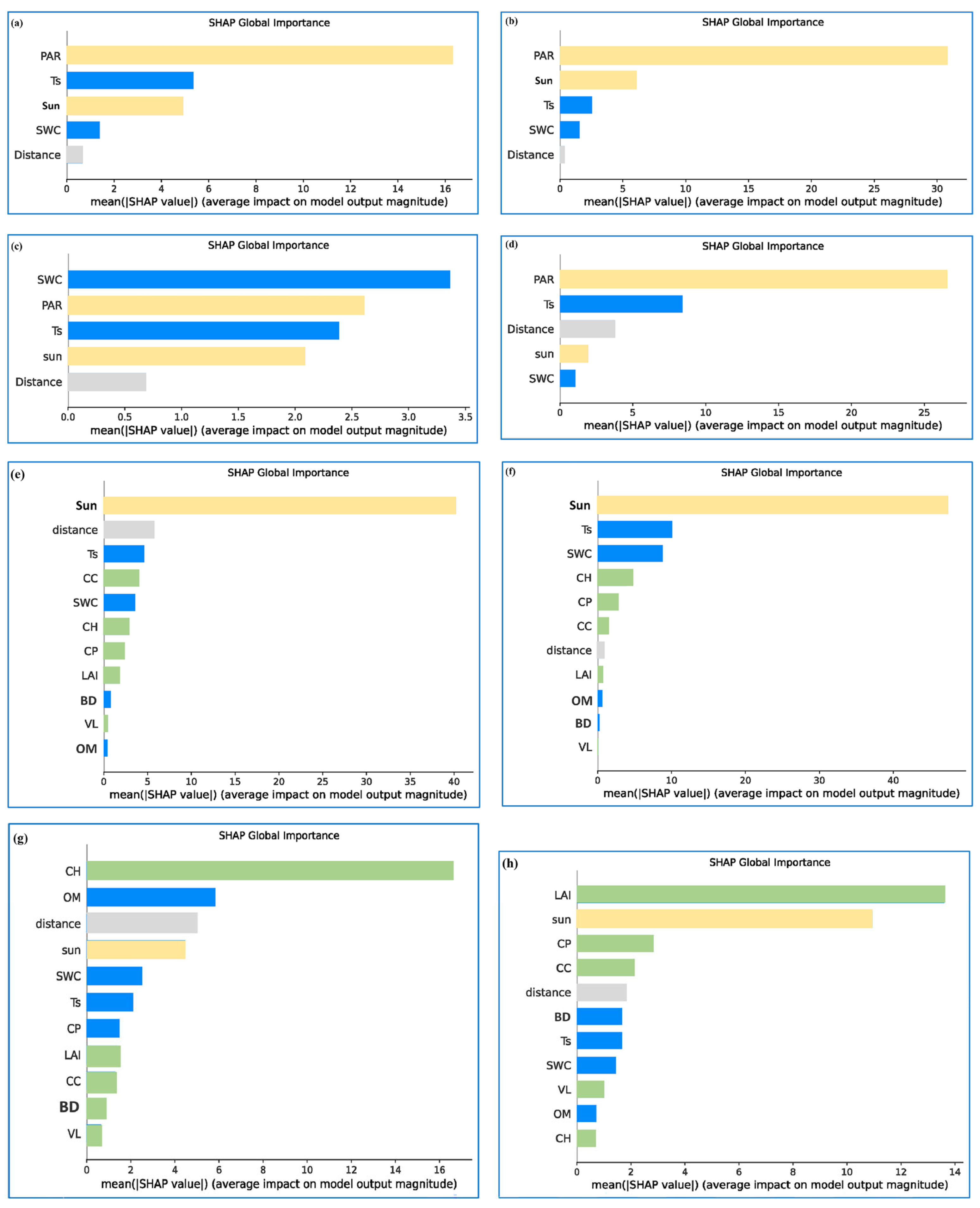
To quantify the relative importance of meteorological, soil, vegetation, and river-related variables in driving H and LE, we applied SHapley Additive exPlanations (SHAP) to the best-performing Random Forest models (Table A3). Figure 16 summarizes the SHAP importance scores for hourly and daily scales in both grassland and forest ecosystems.
In the riparian grassland at the daily scale, PAR emerged as the primary driver, contributing 56.91% to H and 74.49% to LE. Ts followed for H (18.72%), whereas SUN was second for LE (18.72%). Meteorological parameters summed to 74.07% for H and 89.09% for LE, while soil variables (SWC and Ts) provided 23.58% and 9.98%, respectively; distance to the river explained less than 3% in either flux.
Forests displayed a more balanced attribution pattern. On hourly time-steps, SUN dominated both fluxes, yet vegetation structural attributes—canopy height (CH), leaf area index (LAI), canopy closure (CC), canopy porosity (CP), canopy width (CW), and vertical layering (VL)—together accounted for over 50% of annual-scale variability in H and LE. Soil variables (Ts and SWC) exerted markedly stronger influence on LE (25.65%) than on H (9.58%), whereas distance to the river contributed up to 10.19% to H, operating chiefly through its modulation of soil moisture and temperature gradients.
At the annual scale in grassland, soil water content became the leading factor for H (30.29%), followed by PAR (23.39%), Ts (20.19%), and SUN (18.66%); PAR alone dominated LE (63.73%), with Ts contributing a further 20.19%. Thus, soil parameters collectively explained 51.76% of annual H, while meteorological variables explained 68.24% of annual LE. In forests, vegetation attributes surpassed all other categories, summing to 50.75% for H and 52.56% for LE. CH was foremost for H (15.40%), whereas LAI dominated LE (35.28%). Soil variables and meteorological variables each provided roughly 20%–25% of annual fluxes, while distance to the river remained minor (<7%).
Overall, the analyses reveal a clear temporal shift in control: meteorological forcing governs daily heat-flux variability, whereas vegetation structure and soil properties jointly command more than half of the annual energy partitioning, with water-body proximity exerting influence primarily through indirect modification of soil thermal and moisture regimes.

4. Discussion

4.1. Discussion of Daily-Scale Drivers in Riparian Grassland and Forests

In the riparian grassland, the daily energy partitioning is overwhelmingly governed by meteorological conditions. Photosynthetically active radiation exerts the single strongest influence on both sensible and latent heat fluxes, a pattern that concurs with previous work attributing midday surges in evapotranspiration to incident radiation-driven stomatal behavior [57]. The secondary role played by soil temperature reflects the rapid thermal response of the bare or sparsely vegetated surface, while sunshine duration lengthens the effective transpiration window and thereby augments LE [50]. The minor share ascribed to water-body proximity indicates that over a single day, the evapotranspirative demand above short grass is largely decoupled from river-mediated soil moisture anomalies.
For the forested sites, the daily balance is again led by meteorological variables, yet the importance of distance to the river rises sharply for sensible heat flux. This suggests that the horizontal advection of cooler, moister air across the riparian fringe remains significant beneath tall canopies, an interpretation consistent with earlier reports of river-induced temperature gradients persisting under dense foliage [7]. Soil temperature and soil water content emerge as key mediators of latent heat exchange, underpinning the strong physical link between root-zone moisture availability and canopy conductance [36,58]. The dominant role of sunshine duration, however, confirms that even within complex canopies, the instantaneous supply of radiative energy ultimately modulates the magnitude of turbulent fluxes [59].

4.2. Discussion of Annual-Scale Drivers in Riparian Grassland and Forests

On the annual scale, energy partitioning in the riparian grassland is governed by an interplay between soil moisture and meteorological forcing. Soil water content emerges as the single strongest predictor of sensible heat flux, accounting for nearly one-third of its variability. This dominant role is consistent with observations from plantation forests along the upper Lijiang River, where elevated soil moisture increases thermal capacity and heat storage within the soil profile, thereby reducing the upward release of sensible heat [60]. Photosynthetically active radiation and sunshine duration, although secondary, still exert a substantial influence on latent heat flux, together explaining more than four-fifths of its annual variance. This underscores the sustained dependence of grassland evapotranspiration on available energy, even when integrated over an entire year.
In the forested riparian zones, vegetation structure becomes the principal control of both sensible and latent heat exchange. Canopy height is the foremost determinant of sensible heat flux, as taller canopies dampen near-surface wind speed and create a gentler vertical temperature gradient, thereby constraining turbulent transport [61]. The redistribution of radiant energy within deeper canopies further modulates the partitioning between sensible and latent components, a conclusion reinforced by landscape-scale assessments that highlight canopy height as a critical driver of energy exchange [62]. Soil organic matter, although of secondary importance, reduces soil thermal conductivity and thus attenuates sensible heat transfer between the surface and the atmosphere.
Latent heat flux in forests is overwhelmingly shaped by leaf area index, which alone accounts for more than one-third of its annual variability. High LAI increases the effective evaporative surface, enhances canopy conductance, and intercepts additional radiation, all of which elevate transpirational demand [63]. Sunshine duration, canopy porosity, and canopy closure reinforce this effect by influencing both radiation penetration and boundary-layer ventilation [64]. These vegetation attributes operate in concert with seasonal phenology: variations in LAI at leaf-out and senescence periods markedly alter evapotranspiration rates [65], while the overall canopy structure modifies albedo, soil temperature, and soil water content, thereby governing the absorption and subsequent dissipation of energy [66]. Thus, the forest sites exhibit a clear transition from meteorological dominance at short time-steps to biophysical control when aggregated across the annual cycle.

4.3. Limitations

The present study provides a year-round, multi-community assessment of energy exchange within Shanghai’s urban riparian zones. Nevertheless, several limitations should be acknowledged. First, the monitoring period spans only one hydrological year, which may not capture inter-annual variability in precipitation, river stage, or vegetation phenology. Second, the research sites, although representative of common riparian plant assemblages in the region, are restricted to a single river reach with similar revetment type and elevation; this limits the transferability of the derived relationships to rivers with different geometries or flow regimes. Third, eddy-covariance towers were not installed; latent and sensible heat fluxes were instead derived from meteorological gradients and canopy conductance models, introducing uncertainties in absolute flux magnitudes under low-turbulence conditions. Finally, the Random Forest–SHAP framework, while powerful for identifying dominant drivers, remains correlative; controlled manipulations (e.g., irrigation or canopy pruning experiments) are required to confirm causal pathways.
Future research should therefore extend observations to multiple climatic regions and river typologies, ideally incorporating multi-year datasets to test resilience under extreme events such as droughts or heatwaves. Integrating tower-based eddy covariance with distributed soil heat-flux plates would reduce model uncertainty and allow closure of the surface energy balance. Additionally, coupling high-resolution thermal imagery or UAV-based structure-from-motion with ground data could upscale plot-level findings to entire river corridors. Long-term manipulative experiments that systematically vary canopy height, LAI, and soil moisture will ultimately be necessary to validate the biophysical controls identified here and to guide evidence-based design guidelines for climate-adaptive urban riparian landscapes.

5. Conclusions

This study identifies the temporal and spatial variations of sensible and latent heat flux in urban riparian forests and grasslands on both daily and annual scales, and explores their correlations with the river and parameters of vegetation, soil, under the mutual influence of vegetation and water bodies. The results reveal that urban riparian plant communities exhibit pronounced spatiotemporal heterogeneity in sensible (H) and latent heat (LE) fluxes, driven by synergistic water-vegetation interactions. Key findings indicate distinct diurnal and seasonal patterns: LE amplitude exceeded H in summer but reversed in winter, while spatial gradients showed H increasing and LE decreasing with distance from water bodies in grasslands/broadleaf forests—effects attenuated in coniferous canopies due to suppressed turbulent exchange. Interpretable machine learning identified a scale-dependent regulatory mechanism: meteorological parameters dominated daily flux variations, whereas vegetation structural attributes contributed >50% to annual-scale energy partitioning. These findings suggest that optimizing riparian plant configurations can strategically enhance the microclimate regulation function of urban riparian forests. Future research should incorporate multi-year monitoring to assess climate resilience, expand to diverse climatic zones, and expand ecosystem coverage to include more diverse riparian types.

Author Contributions

Conceptualization, Y.Q., C.Y. and A.L.; methodology, Y.Q. and C.Y.; software, Y.Q. and A.L.; validation, Y.Q., C.Y. and A.L.; formal analysis, C.X. and Y.Z.; investigation, Y.Q. and J.W.; resources, C.X. and Y.Z.; data curation, J.W.; writing—original draft preparation, Y.Q., C.Y. and A.L.; writing—reviewing and editing, C.X. and S.C.; visualization, Y.Q. and A.L.; supervision, S.C.; project administration, C.X.; funding acquisition, C.X. and S.C. All authors have read and agreed to the published version of the manuscript.

Funding

This research was supported by the Guilin City Scientific Research and Technological Development Program Project (Grand No.: 20230127-3), Shanghai Municipality’s Action Plan for Science and Technology Innovation-International Science and Technology Cooperation Project [Grant No. 22230750500], and Shanghai Jiao Tong University Research Startup Project [Grant No. WH220443004].

Data Availability Statement

The data presented in this study are available upon request from the author.

Acknowledgments

The authors are grateful to the editor and reviewers for their valuable comments and suggestions.

Conflicts of Interest

The authors declare no conflicts of interest.

Abbreviations

The following abbreviations are used in this manuscript:
Hsensible heat flux
LElatent heat fluxes
LAIleaf area index
CCcanopy closure
CPcanopy porosity
Tssoil temperature
SWCsoil water content
VPDwater pressure deficit
uwind speed
Rnnet radiation
PARphotosynthetically active radiation
SUNsunshine duration
THtree height
CHcanopy height
CWcanopy width
VLvertical layering
SOMsoil organic matter

Appendix A

Table A1. Monthly Leaf Index Area (LAI), canopy porosity (CP), and canopy closure (CC) of six canopied riparian plant communities.
Heat FluxesMonthCCO·CMOCCHCUOCMHCUH
CC159.7061.2058.9065.5065.9062.90
255.6065.4065.4062.6067.1065.80
350.1066.0262.8465.2869.9561.28
452.3061.9054.2050.4063.4047.80
554.4543.0226.0053.0151.4728.52
653.2040.7049.8048.5053.7030.56
754.4541.9653.0126.0051.4728.52
867.8249.0651.4653.5367.8341.16
953.7556.1057.0763.4773.2064.77
1057.3059.6059.1065.8075.8063.90
1164.6064.8060.5069.4073.7065.60
1265.8467.1363.7163.5269.2567.15
LAI11.682.322.042.052.642.67
21.652.291.641.801.611.49
31.642.361.531.411.211.23
41.751.541.671.131.030.80
51.860.791.240.500.790.50
61.350.861.090.571.040.53
70.951.141.030.661.100.51
81.521.671.120.992.081.19
91.772.001.531.573.551.51
101.582.871.691.913.641.84
111.813.111.832.233.822.49
121.693.222.102.453.952.49
CP110.5315.3821.849.3818.4917.47
211.3615.9223.528.4717.3019.43
39.0113.9021.336.1010.3820.13
410.8719.0625.7410.5620.5426.50
510.3730.5423.0518.9843.6139.14
610.5630.8629.5422.0342.7340.30
710.3730.5426.1823.0543.6139.14
821.1828.8843.5718.3028.1831.53
910.5020.5615.3712.0615.499.90
1010.9314.4719.2814.6313.2015.92
119.4516.7218.4512.9516.7114.31
1210.1715.5920.2710.5418.7322.35
Table A2. Percentages of missing data and outliers in each riparian plant community (%).
Parameter/SiteCCO·CMOCHCCHCUOCMHCUH
PAR//10.95//4.30/
Net radiation//11.12//4.30/
Sunshine duration//////8.22
Air temperature1 m-to-river1.108.221.084.936.853.012.19
6 m-to-river4.660.552.745.485.481.373.29
11 m-to-river9.862.744.935.750.825.752.10
Air relative humidity1 m-to-river1.108.221.084.936.853.012.19
6 m-to-river4.660.552.745.485.481.373.29
11 m-to-river9.862.744.935.750.825.752.10
Wind speed1 m-to-river1.108.221.084.936.852.472.19
6 m-to-river4.661.092.471.101.100.553.29
11 m-to-river6.851.924.930.550.826.032.15
Soil temperature1 m-to-river/0.554.11/6.856.5811.16
6 m-to-river8.490.554.11/5.480.82/
11 m-to-river8.2210.960.270.820.55/4.11
Soil water content1 m-to-river/0.554.11/6.857.678.49
6 m-to-river8.496.854.11/2.741.10/
11 m-to-river8.2210.9613.677.950.550.274.11
Table A3. Fitting Parameters of five models of sensible heat flux (H) and latent heat flux (LE) in different riparian sites.
Heat FluxTemporal ScalesRiparian SitesModelR2RMSEMAE
HDailyGrasslandRandom Forest0.9535.3933.222
XGBoost0.9495.6393.240
MLP0.9386.2234.022
SVR0.9077.6254.340
LightGBM0.8888.3634.944
ForestsRandom Forest0.65114.5266.091
XGBoost0.60316.8317.671
LightGBM0.59517.2518.960
MLP0.58123.8749.118
SVR0.50126.29213.808
AnnualGrasslandRandom Forest0.76410.3556.236
LightGBM0.71911.3956.166
SVR0.71711.3976.130
MLP0.59516.50513.308
XGBoost0.26416.79213.566
ForestsRandom Forest0.68113.4817.711
MLP0.66313.9638.178
LightGBM0.65814.1118.002
XGBoost0.65214.2578.360
SVR0.63914.6028.659
LEDailyGrasslandRandom Forest0.9607.2785.004
XGBoost0.9468.4985.666
MLP0.9458.5305.514
SVR0.90511.2656.457
LightGBM0.89511.7976.089
ForestsRandom Forest0.78112.0167.432
XGBoost0.71716.2917.067
LightGBM0.69217.8639.929
MLP0.65122.36311.877
SVR0.61222.56911.198
AnnualGrasslandRandom Forest0.9607.2785.004
LightGBM0.9468.4985.666
SVR0.9458.5305.514
MLP0.90511.2656.457
XGBoost0.89511.7976.089
ForestsRandom Forest0.77610.2746.563
MLP0.75710.8606.921
LightGBM0.75610.9016.987
XGBoost0.74610.1927.014
SVR0.72610.7767.333
Figure A1. Diurnal variations of environmental conditions in CCH during three consecutive sunny days in each season—winter (a), spring (b), summer (c), and autumn (d). VPD: vapor-pressure deficit; PAR: photosynthetically active radiation; Ta: air temperature; Ts: soil temperature; SWC: soil water content; u: wind speed.
Forests 16 01466 g0a1
Figure A2. Diurnal variations of environmental conditions in CMO during three consecutive sunny days in each season—winter (a), spring (b), summer (c), and autumn (d). VPD: vapor-pressure deficit; PAR: photosynthetically active radiation; Ta: air temperature; Ts: soil temperature; SWC: soil water content; u: wind speed.
Forests 16 01466 g0a2
Figure A3. Diurnal variations of environmental conditions in CMH during three consecutive sunny days in each season—winter (a), spring (b), summer (c), and autumn (d). VPD: vapor-pressure deficit; PAR: photosynthetically active radiation; Ta: air temperature; Ts: soil temperature; SWC: soil water content; u: wind speed.
Forests 16 01466 g0a3
Figure A4. Diurnal variations of environmental conditions in CUO during three consecutive sunny days in each season—winter (a), spring (b), summer (c), and autumn (d). VPD: vapor-pressure deficit; PAR: photosynthetically active radiation; Ta: air temperature; Ts: soil temperature; SWC: soil water content; u: wind speed.
Forests 16 01466 g0a4
Figure A5. Diurnal variations of environmental conditions in CUH during three consecutive sunny days in each season—winter (a), spring (b), summer (c), and autumn (d). VPD: vapor-pressure deficit; PAR: photosynthetically active radiation; Ta: air temperature; Ts: soil temperature; SWC: soil water content; u: wind speed.
Forests 16 01466 g0a5
Figure A6. Diurnal variations of environmental conditions in CCO during three consecutive sunny days in each season—winter (a), spring (b), summer (c), and autumn (d). VPD: vapor-pressure deficit; PAR: photosynthetically active radiation; Ta: air temperature; Ts: soil temperature; SWC: soil water content; u: wind speed.
Forests 16 01466 g0a6
Figure A7. Seasonal variations of environmental parameters in CH, VPD: vapor-pressure deficit, sun: sunshine duration, PAR: photosynthetically active radiation, Ta: air temperature, Ts: soil temperature, SWC: soil water content.
Forests 16 01466 g0a7
Figure A8. Seasonal variations of environmental parameters in CCH, VPD: vapor-pressure deficit, sun: sunshine duration, PAR: photosynthetically active radiation, Ta: air temperature, Ts: soil temperature, SWC: soil water content.
Forests 16 01466 g0a8
Figure A9. Seasonal variations of environmental parameters in CMO, VPD: vapor-pressure deficit, sun: sunshine duration, PAR: photosynthetically active radiation, Ta: air temperature, Ts: soil temperature, SWC: soil water content.
Forests 16 01466 g0a9
Figure A10. Seasonal variations of environmental parameters in CMH, VPD: vapor-pressure deficit, sun: sunshine duration, PAR: photosynthetically active radiation, Ta: air temperature, Ts: soil temperature, SWC: soil water content.
Forests 16 01466 g0a10
Figure A11. Seasonal variations of environmental parameters in CUO, VPD: vapor-pressure deficit, sun: sunshine duration, PAR: photosynthetically active radiation, Ta: air temperature, Ts: soil temperature, SWC: soil water content.
Forests 16 01466 g0a11
Figure A12. Seasonal variations of environmental parameters in CUH, VPD: vapor-pressure deficit, sun: sunshine duration, PAR: photosynthetically active radiation, Ta: air temperature, Ts: soil temperature, SWC: soil water content.
Forests 16 01466 g0a12

References

  1. Yu, Z.; Yang, G.; Zuo, S.; Gertrud, J.; Motoya, K.; Henrik, V. Critical review on the cooling effect of urban blue-green space: A threshold-size perspective. Urban For. Urban Green. 2020, 49, 126630. [Google Scholar] [CrossRef]
  2. Wang, K.; Dickinson, R.E. A review of global terrestrial evapotranspiration: Observation, modeling, climatology, and climatic variability: Global terrestrial evapotranspiration. Rev. Geophys. 2012, 50, RG2005. [Google Scholar] [CrossRef]
  3. Ballinger, A.; Lake, P.S. Energy and nutrient fluxes from rivers and streams into terrestrial food webs. Mar. Freshw. Res. 2006, 57, 15. [Google Scholar] [CrossRef]
  4. Oettel, J.; Braun, M.; Sallmannshofer, M.; De Groot, M.; Schueler, S.; Virgillito, C.; Westergren, M.; Božič, G.; Nagy, L.; Stojnić, S.; et al. River distance, stand basal area, and climatic conditions are the main drivers influencing lying deadwood in riparian forests. For. Ecol. Manag. 2022, 520, 520120415. [Google Scholar] [CrossRef]
  5. Cai, Z.; Han, G.; Chen, M. Do water bodies play an important role in the relationship between urban form and land surface temperature? Sustain. Cities Soc. 2018, 39, 487–498. [Google Scholar] [CrossRef]
  6. Ballinas, M.; Barradas, V.L. Transpiration and stomatal conductance as potential mechanisms to mitigate the heat load in Mexico City. Urban For. Urban Green. 2016, 20, 152–159. [Google Scholar] [CrossRef]
  7. Garner, G.; Malcolm, I.A.; Sadler, J.P.; Millar, C.P.; Hannah, D.M. Inter-annual variability in the effects of riparian woodland on micro-climate, energy exchanges and water temperature of an upland Scottish stream. Hydrol. Process. 2015, 29, 1080–1095. [Google Scholar] [CrossRef]
  8. Salata, F.; Golasi, I.; Petitti, D.; Emanuele de, L.V.; Massimo, C.; Andrea, L.V.d. Relating microclimate, human thermal comfort and health during heat waves: An analysis of heat island mitigation strategies through a case study in an urban outdoor environment. Sustain. Cities Soc. 2017, 30, 79–96. [Google Scholar] [CrossRef]
  9. Kumagai, T.; Saitoh, T.M.; Sato, Y.; Toshiyuki, M.; Odair, J.M.; Koichiro, K.; Masakazu, S. Transpiration, canopy conductance and the decoupling coefficient of a lowland mixed dipterocarp forest in Sarawak, Borneo: Dry spell effects. J. Hydrol. 2004, 287, 237–251. [Google Scholar] [CrossRef]
  10. Leuning, R. Estimation of scalar source/sink distributions in plant canopies using lagrangian dispersion analysis: Corrections for atmospheric stability and comparison with a multilayer canopy model. Bound. Layer Meteorol. 2000, 96, 293–314. [Google Scholar] [CrossRef]
  11. Wang, A. Estimation of water vapor source/sink distribution and evapotranspiration over broadleaved Koreanpine forest in Changbai Mountain using inverse Lagrangian dispersion analysis. Geophys. Res. 2005, 110, D08102. [Google Scholar] [CrossRef]
  12. Zhang, S.Y.; Li, X.Y.; Ma, Y.J.; Guo, Q.Z.; Liu, L.; Ji, C.; Zhi, Y.J.; Yong, M.H. Interannual and seasonal variability in evapotranspiration and energy partitioning over the alpine riparian shrub Myricaria squamosa Desv. on Qinghai–Tibet Plateau. Cold Reg. Sci. Technol. 2014, 102, 8–20. [Google Scholar] [CrossRef]
  13. Kan, Y.; Shao, H.; Yao, Y.; Li, Y.; Zhang, X.; Xu, J.; Zhang, X.; Xie, Z.; Ning, J.; Yu, R.; et al. Evaluation of two strategies from the SEBS model for estimating the daily terrestrial evapotranspiration values of the Tibetan Plateau. J. Hydrol. 2025, 656, 132921. [Google Scholar] [CrossRef]
  14. Mingyue, Z.; Guojie, W.; Hagan, D.F.T.; Waheed, U.; Giri, K.; Jiao, L.; ShiJie, L. Impacts of Vegetation Changes on Land Evapotranspiration in China During 1982–2015. Front. Environ. Sci. 2022, 10, 819277. [Google Scholar] [CrossRef]
  15. Hu, Z.; Yu, G.; Zhou, Y.; Sun, X.; Li, Y.; Peili, S.; Wang, Y.; Xia, S.; Zemei, Z.; Li, Z.; et al. Partitioning of evapotranspiration and its controls in four grassland ecosystems: Application of a two-source model. Agric. For. Meteorol. 2009, 149, 1410–1420. [Google Scholar] [CrossRef]
  16. Wang, Q.-W.; Robson, T.M.; Pieristè, M.; Kenta, T.; Zhou, W.; Kurokawa, H. Canopy structure and phenology modulate the impacts of solar radiation on C and N dynamics during litter decomposition in a temperate forest. Sci. Total Environ. 2022, 820, 153185. [Google Scholar] [CrossRef]
  17. Miri, A.; Dragovich, D.; Dong, Z. The response of live plants to airflow—Implication for reducing erosion. Aeolian Res. 2018, 33, 93–105. [Google Scholar] [CrossRef]
  18. Ma, W.; Yu, Z.; Chen, J.; Yang, W.; Zhang, Y.; Hu, Y.; Shao, M.; Hu, J.; Zhang, Y.; Zhang, H.; et al. What drives the cooling dynamics of urban vegetation via evapotranspiration and shading under extreme heat? Sustain. Cities Socities 2025, 130, 106659. [Google Scholar] [CrossRef]
  19. Best, L.; Schwarz, N.; Obergh, D.; Teuling, A.J.; Van Kanten, R.; Willemen, L. Urban green spaces and variation in cooling in the humid tropics: The case of Paramaribo. Urban For. Urban Green. 2023, 89, 128111. [Google Scholar] [CrossRef]
  20. Alonzo, M.; Ibsen, P.C.; Locke, D.H. Urban Trees and Cooling: A Review of the Recent Literature (2018 to 2024). Arboric. Urban For. 2025, 51, 1–24. [Google Scholar] [CrossRef]
  21. Zhou, J.; Yang, K.; Crow, W.T.; Dong, J.; Zhao, L.; Feng, H.; Zou, M.; Lu, H.; Tang, R.; Jiang, Y. Potential of remote sensing surface temperature- and evapotranspiration-based land-atmosphere coupling metrics for land surface model calibration. Remote Sens. Environ. 2023, 291, 113557. [Google Scholar] [CrossRef]
  22. Detommaso, M.; Costanzo, V.; Nocera, F. Application of weather data morphing for calibration of urban ENVI-met microclimate models. Results and critical issues. Urban Clim. 2021, 38, 100895. [Google Scholar] [CrossRef]
  23. Brozovsky, J.; Simonsen, A.; Gaitani, N. Validation of a CFD model for the evaluation of urban microclimate at high latitudes: A case study in Trondheim, Norway. Build. Environ. 2021, 205, 108175. [Google Scholar] [CrossRef]
  24. Schöneberger, P.; Sinsel, T.; Ouyang, W.; Tan, Z.; Bruse, M.; Simon, H. Enhancing urban microclimate simulations: Validating ENVI-met’s accuracy in modeling multi-directional radiative fluxes and mean radiant temperature in subtropical hong kong. Build. Environ. 2025, 284, 113475. [Google Scholar] [CrossRef]
  25. Yu, Z.; Chen, J.; Chen, J.; Zhan, W.; Wang, C.; Ma, W.; Yao, X.; Zhou, S.; Zhu, K.; Sun, R. Enhanced observations from an optimized soil-canopy-photosynthesis and energy flux model revealed evapotranspiration-shading cooling dynamics of urban vegetation during extreme heat. Remote Sens. Environ. 2025, 305, 114098. [Google Scholar] [CrossRef]
  26. Zhang, Q.; Jia, B.; Li, T.; Yang, Y.; Fang, Y. Dynamic changes and drives of surface urban heat islands in China. City Environ. Interact. 2025, 27, 100203. [Google Scholar] [CrossRef]
  27. Liang, A.; Xie, C.; Wang, J.; Che, S. Daily Dynamics of Soil Heat Flux and Its Relationship with Net Radiation in Different Urban Riparian Woodlands. Forests 2022, 13, 2062. [Google Scholar] [CrossRef]
  28. Dong, J.; Wu, L.; Zeng, W.; Xiao, X.; He, J. Analysis of spatial-temporal trends and causes of vapor pressure deficit in China from 1961 to 2020. Atmos. Res. 2024, 299, 107199. [Google Scholar] [CrossRef]
  29. Guenther, S.M.; Moore, R.D.; Gomi, T. Riparian microclimate and evaporation from a coastal headwater stream, and their response to partial-retention forest harvesting. Agric. For. Meteorol. 2012, 164, 1–9. [Google Scholar] [CrossRef]
  30. Ma, N.; Zhang, Y.; Guo, Y.; Gao, H.; Zhang, H.; Wang, Y. Environmental and biophysical controls on the evapotranspiration over the highest alpine steppe. J. Hydrol. 2015, 529, 980–992. [Google Scholar] [CrossRef]
  31. Ma, J.; Zha, T.; Jia, X.; Tian, Y.; Bourque, C.P.; Bourque, C.P.; Liu, P.; Bai, Y.; Wu, Y.; Ren, C.L.; et al. Energy and water vapor exchange over a young plantation in northern China. Agric. For. Meteorol. 2018, 263, 334–345. [Google Scholar] [CrossRef]
  32. Sommer, R.; Sá TDde, A.; Vielhauer, K.; de Araújo, A.C.; Fölster, H.; Vlek, P.L. Transpiration and canopy conductance of secondary vegetation in the eastern Amazon. Agric. For. Meteorol. 2002, 112, 103–121. [Google Scholar] [CrossRef]
  33. Matsumoto, K.; Ohta, T.; Tanaka, T. Dependence of stomatal conductance on leaf chlorophyll concentration and meteorological variables. Agric. For. Meteorol. 2005, 132, 44–57. [Google Scholar] [CrossRef]
  34. Brenner, A.J.; Incoll, L.D. The effect of clumping and stomatal response on evaporation from sparsely vegetated shrublands. Agric. For. Meteorol. 1997, 84, 187–205. [Google Scholar] [CrossRef]
  35. Dupont, S.; Patton, E.G. Influence of stability and seasonal canopy changes on micrometeorology within and above an orchard canopy: The CHATS experiment. Agric. For. Meteorol. 2012, 157, 11–29. [Google Scholar] [CrossRef]
  36. Liu, X.; Yang, S.; Xu, J.; Zhang, J.; Liu, J. Effects of soil heat storage and phase shift correction on energy balance closure of paddy fields. Atmósfera 2017, 30, 39–52. [Google Scholar] [CrossRef]
  37. Azevedo, B.F.; Rocha, A.M.A.C.; Pereira, A.I. Hybrid approaches to optimization and machine learning methods: A systematic literature review. Mach. Learn. 2024, 113, 4055–4097. [Google Scholar] [CrossRef]
  38. Shi, D.; Song, J.; Huang, J.; Zhuang, C.; Guo, R.; Gao, Y. Synergistic cooling effects (SCEs) of urban green-blue spaces on local thermal environment: A case study in Chongqing, China. Sustain. Cities Soc. 2020, 55, 102065. [Google Scholar] [CrossRef]
  39. Hathway, E.A.; Sharples, S. The interaction of rivers and urban form in mitigating the Urban Heat Island effect: A UK case study. Build. Environ. 2012, 58, 14–22. [Google Scholar] [CrossRef]
  40. Linscheid, N.; Estupinan-Suarez, L.M.; Brenning, A.; Carvalhais, N.; Cremer, F.; Gans, F.; Rammig, A.; Reichstein, M.; Sierra, C.A.; Mahecha, M.D. Towards a global understanding of vegetation–climate dynamics at multiple timescales. Biogeosciences 2020, 17, 945–962. [Google Scholar] [CrossRef]
  41. Behera, S.K.; Mishra, A.K.; Sahu, N.; Kumar, A.; Singh, N.; Kumar, A.; Bajpai, O.; Chaudhary, L.B.; Khare, P.B.; Tuli, R. The study of microclimate in response to different plant community association in tropical moist deciduous forest from northern India. Biodivers. Conserv. 2012, 21, 1159–1176. [Google Scholar] [CrossRef]
  42. Liu, H.; Zhang, Q.; Dowler, G. Environmental controls on the surface energy budget over a large southern inland water in the United States: An analysis of one-year eddy covariance flux data. J. Hydrometeorol. 2012, 13, 1893–1910. [Google Scholar] [CrossRef]
  43. Yu, Z.; Chen, T.; Yang, G.; Sun, R.; Xie, W.; Vejre, H. Quantifying seasonal and diurnal contributions of urban landscapes to heat energy dynamics. Appl. Energy 2020, 264, 114724. [Google Scholar] [CrossRef]
  44. Gao, Z.; Lenschow, D.H.; He, Z.; Zhou, M.; Wang, L.Y.; Wang, Y.H.; He, J. Seasonal and diurnal variations in moisture, heat and CO2 fluxes over a typical steppe prairie in Inner Mongolia, China. Hydrol. Earth Syst. Sci. 2009, 6, 987–998. [Google Scholar] [CrossRef]
  45. Zhao, X.; Liu, Y. Phase transition of surface energy exchange in China’s largest freshwater lake. Agric. For. Meteorol. 2017, 244, 98–110. [Google Scholar] [CrossRef]
  46. Lenters, J.D.; Cutrell, G.J.; Istanbulluoglu, E.; Scott, D.T.; Herrman, K.S.; Irmak, A.; Eisenhauer, D.E. Seasonal energy and water balance of a Phragmites australis-dominated wetland in the Republican River basin of south-central Nebraska (USA). J. Hydrol. 2011, 408, 19–34. [Google Scholar] [CrossRef]
  47. Wang, L.; Gao, Z.; Pan, Z.; Guo, X.; Bou-Zeid, E. Evaluation of Turbulent Surface Flux Parameterizations over Tall Grass in a Beijing Suburb. J. Hydrometeorol. 2013, 14, 1620–1635. [Google Scholar] [CrossRef]
  48. Wang, Y.; You, C.; Tan, X.; Ren, T.; Su, T.; Han, X.; Chen, S. Co-regulation of climate and vegetation on seasonal and interannual variations of energy exchange over a temperate grassland. Agric. For. Meteorol. 2025, 369, 110556. [Google Scholar] [CrossRef]
  49. Zhou, L.T.; Huang, R. Regional differences in surface sensible and latent heat fluxes in China. Theor. Appl. Climatol. 2014, 116, 625–637. [Google Scholar] [CrossRef]
  50. Xu, C.; Huang, Q.; Haase, D.; Dong, Q.; Teng, Y.; Su, M.; Yang, Z. Cooling Effect of Green Spaces on Urban Heat Island in a Chinese Megacity: Increasing Coverage versus Optimizing Spatial Distribution. Environ. Sci. Technol. 2024, 58, 5811–5820. [Google Scholar] [CrossRef]
  51. Yuan, G.; Zhang, P.; Shao, M.; Luo, Y.; Zhu, X. Energy and water exchanges over a riparian Tamarix spp. stand in the lower Tarim River basin under a hyper-arid climate. Agric. For. Meteorol. 2014, 194, 144–154. [Google Scholar] [CrossRef]
  52. Kovács, B.; Tinya, F.; Ódor, P. Stand structural drivers of microclimate in mature temperate mixed forests. Agric. For. Meteorol. 2017, 234, 11–21. [Google Scholar] [CrossRef]
  53. Stephens, C.M.; Lall, U.; Johnson, F.M.; Marshall, L.A. Landscape changes and their hydrologic effects: Interactions and feedbacks across scales. Earth Sci. Rev. 2021, 212, 103466. [Google Scholar] [CrossRef]
  54. Olson, D.H.; Anderson, P.D.; Frissell, C.A.; Welsh, H.H.; Bradford, D.F. Biodiversity management approaches for stream–riparian areas: Perspectives for Pacific Northwest headwater forests, microclimates, and amphibians. For. Ecol. Manag. 2007, 246, 81–107. [Google Scholar] [CrossRef]
  55. Welsh, H.H.; Hodgson, G.R.; Karraker, N.E. Influences of the vegetation mosaic on riparian and stream environments in a mixed forest-grassland landscape in “Mediterranean” northwestern California. Ecography 2005, 28, 537–551. [Google Scholar] [CrossRef]
  56. Rambo, T.; North, M. Spatial and temporal variability of canopy microclimate in a Sierra Nevada riparian forest. Northwest Sci. 2008, 82, 259–268. [Google Scholar] [CrossRef]
  57. Lin, P.-A.; Chen, Y.; Ponce, G.; Acevedo, F.E.; Lynch, J.P.; Anderson, C.T.; Ali, J.G.; Felton, G.W. Stomata-mediated interactions between plants, herbivores, and the environment. Trends Plant Sci. 2022, 27, 287–300. [Google Scholar] [CrossRef]
  58. Su, W.; Charlock, T.P.; Rose, F.G.; Rutan, D. Photosynthetically active radiation from Clouds and the Earth’s Radiant Energy System (CERES) products. J. Geophys. Res. 2007, 112, G02022. [Google Scholar] [CrossRef]
  59. Chen, S.; Wei, W.; Tong, B.; Chen, L. Effects of soil moisture and vapor pressure deficit on canopy transpiration for two coniferous forests in the Loess Plateau of China. Agric. For. Meteorol. 2023, 339, 109581. [Google Scholar] [CrossRef]
  60. Wang, X.; Wang, P.; Zhu, Q. Spatio-temporal variation of water and heat fluxes over complex hilly topography in upper reaches of Lijiang river. Trans. Chin. Soc. Agric. Eng. 2012, 28, 118–122. [Google Scholar]
  61. Parker, G.G.; Harmon, M.E.; Lefsky, M.A.; Chen, J.; Pelt, R.V.; Weis, S.B.; Thomas, S.C.; Winner, W.E.; Shaw, D.C.; Frankling, J.F. Three-dimensional Structure of an Old-growth Pseudotsuga-Tsuga Canopy and Its Implications for Radiation Balance, Microclimate, and Gas Exchange. Ecosystems 2004, 7, 440–453. [Google Scholar] [CrossRef]
  62. Friedrich, K.; Mlders, N.; Tetzlaff, G. On the Influence of Surface Heterogeneity on the Bowen-Ratio: A Theoretical Case Study. Theor. Appl. Climatol. 2000, 65, 181–196. [Google Scholar] [CrossRef]
  63. Liu, X.; Feng, Y.; Hu, T.; Luo, Y.; Zhao, X.; Wu, J.; Maeda, E.E.; Ju, W.; Liu, L.; Guo, Q.; et al. Enhancing ecosystem productivity and stability with increasing canopy structural complexity in global forests. Sci. Adv. 2024, 10, 14. [Google Scholar] [CrossRef] [PubMed]
  64. Liu, Z.; Zhao, B.; Yan, H.; Su, J. Energy Partitioning and Latent Heat Flux Driving Factors of the CAM Plant Pineapple (Ananas comosus (L.) Merril) Grown South Subtropical China. Plants 2024, 13, 21. [Google Scholar] [CrossRef]
  65. Scott, R.; Edwards, E.A.; Shuttleworth, W.; Huxman, T.E.; Watts, C.J.; Goodrich, D. Interannual and seasonal variation in fluxes of water and carbon dioxide from a riparian woodland ecosystem. Agric. For. Meteorol. 2004, 122, 65–84. [Google Scholar] [CrossRef]
  66. Beringer, J.; Chapin, F.S.; Thompson, C.C.; Mcguire, A.D. Surface energy exchanges along a tundra-forest transition and feedbacks to climate. Agric. For. Meteorol. 2005, 131, 143–161. [Google Scholar] [CrossRef]
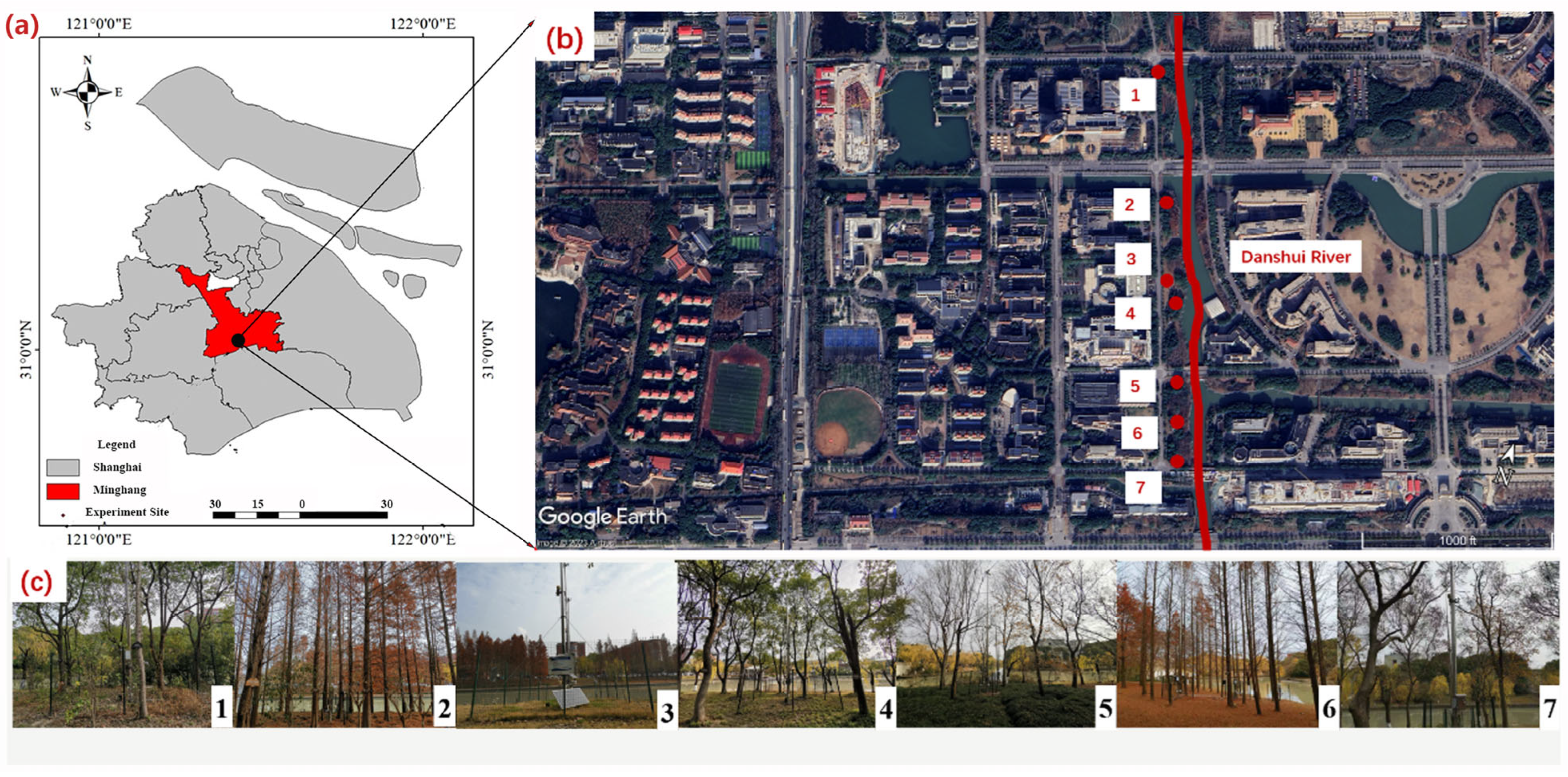
Figure 1. The location of seven riparian sites along the Danshui River in Minhang District, Shanghai (a,b)—CCO (1), CMO (2), CH (3), CCH (4), CUO (5), CMH (6), and CUH (7), and (c) sites photos taken by authors.
Forests 16 01466 g001
Figure 2. The schematic diagram of the south-facing slope of the study transect in sites along the Danshui River (taking the site of arbor-shrub-grass as an example) and a diagram of how the monitoring system operates. Approximate sensor locations are shown with red letters.
Forests 16 01466 g002
Figure 3. Diurnal variations of environmental parameters in CH during three consecutive sunny days in each season—winter (a), spring (b), summer (c), and autumn (d). VPD: vapor-pressure deficit; PAR: photosynthetically active radiation; Ta: air temperature; Ts: soil temperature; SWC: soil water content; u: wind speed.
Forests 16 01466 g003
Figure 4. Seasonal variations of environmental parameters in CCO, VPD: vapor-pressure deficit, sun: sunshine duration, PAR: photosynthetically active radiation, Ta: air temperature, Ts: soil temperature, SWC: soil water content.
Forests 16 01466 g004
Figure 5. Diurnal variations of air temperature (Ta) at different distances to the river within each riparian plant community on sunny days in spring (a), summer (b), autumn (c), and winter (d). From left to right: CCO, CMO, CH, CCH, CUO, CMH, CUH.
Forests 16 01466 g005
Figure 6. Diurnal variations of wind speed (u) at different distances to the river within each riparian plant community on sunny days in spring (a), summer (b), autumn (c), and winter (d).
Forests 16 01466 g006
Figure 7. Diurnal variations of soil temperature (Ts) at different distances to the river within each riparian plant community on sunny days in spring (a), summer (b), autumn (c), and winter (d).
Forests 16 01466 g007
Figure 8. Diurnal variations of soil water content (SWC) 0–30 cm below the soil at 1 m, 6 m, and 11 m to the river in each riparian plant community on sunny days in spring (a), summer (b), autumn (c), and winter (d).
Forests 16 01466 g008
Figure 9. Diurnal variations of vapor pressure deficit (VPD) at different distances to the river within each riparian site on sunny days in spring (a), summer (b), autumn (c), and winter (d).
Forests 16 01466 g009
Figure 10. Seasonal variations of vapor pressure deficit (VPD), air temperature (Ta), soil temperature (Ts), and soil water content (SWC) at different distances to the river within CCO.
Forests 16 01466 g010
Figure 11. Diurnal variations in sensible heat flux (H) and latent heat flux (LE) in seven riparian communities, in spring, summer, autumn, and winter. The bars show the standard deviations.
Forests 16 01466 g011
Figure 12. Annual variation trends of daily averaged latent heat flux (LE) in seven riparian communities.
Forests 16 01466 g012
Figure 13. Diurnal variations (a) of sensible heat flux (H) at different distances from the river in each site in four seasons.
Forests 16 01466 g013
Figure 14. Diurnal variations (a) of latent heat flux (LE) at different distances from the river in each site in four seasons.
Forests 16 01466 g014
Figure 15. Seasonal variations in sensible heat flux (left) and latent heat flux (right) measured at 1 m, 6 m, and 11 m from the river in seven riparian plant communities. Lines indicate a 15-day moving average of daily values.
Forests 16 01466 g015
Figure 16. SHAP importance plot of various variables for hourly H (a) and LE (b), daily H (c) and LE (d) in riparian grassland and for hourly H (e) and LE (f), daily H (g) and LE (h) in riparian forests, in which green bar: vegetation parameters, blue bar: soil parameters, grey: water body and yellow: meteorological parameters.
Forests 16 01466 g016
Table 1. Six riparian plant communities along the Danshui River, Shanghai (LAI is leaf area index).
No.CCOCMOCCHCUOCMHCUHCH
Plant
type
Evergreen broadleaf
arbor-shrub-grass
Coniferous arbor
-shrub-grass
Evergreen broadleaf arbor-grassDeciduous broadleaf arbor-shrub-grassConiferous arbor
-grass
Deciduous broadleaf arbor-grassGrassland
Dominant speciesCinnamomum camphora (L.) J. Presl
Osmanthus fragrans (Thunb.) Lour.
Oxalis corniculate L.
Metasequoia glyptostroboides Hu and W. C. Cheng
Osmanthus fragrans (Thunb.) Lour.
Ophiopogon japonicus (L. f.) Ker Gawl.
Cinnamomum camphora (L.) J. Presl
Osmanthus fragrans (Thunb.) Lour. (Thunb.) Lour.
Ulmus parvifolia Jacq.
Osmanthus fragrans (Thunb.) Lour.
Ophiopogon japonicus (L. f.) Ker Gawl.
Metasequoia glyptostroboides Hu and W. C. Cheng
Zoysia japonica Steud.
Ulmus parvifolia Jacq.
Oxalis corniculate L.
Zoysia japonica Steud.
Trifolium repens L.
Density (/hm2)3751050325400850400/
Height (m)9.7612.809.809.6013.009.040.3
Soil typeLoamyLoamySandy loamSandy loamSandy loamloamySandy loam
Soil organic matter (g/kg)19.6729.7324.9715.56.1118.9322.3
Table 2. Parameters of each sensor and its location.
ParametersUnitInstrumentModelAccuracyHeight (m)Distance-to-River (m)
Net radiationW/m2Net radiometerCNR4, Kipp and Zonen, Delft, The Netherlands±5%10/126
Sunshine durationhSunshine duration sensorCSD3, Kipp and Zonen, Delft, The Netherlands±3%10/126
Photosynthetically active radiationμmol/m2/sPhotosynthetically active radiation sensorPQS1, Kipp and Zonen, Delft, The Netherlands±5%10/126
Wind speedm/sWind speed sensorJXBS-3001, JXCT, Weihai, China±1 m/s0.5, 4, 10/121, 6, 11
Air temperatureAir temperature and humidity sensorRS-BYQXZ-M-1, Renke Control Technology, Jinan, China0.1 °C0.5, 4, 10/121, 6, 11
Relative humidity%RS-BYQXZ-M-1, Renke Control Technology, Jinan, China0.1%0.5, 4, 10/121, 6, 11
Soil water content%Soil temperature and humidity probesRS-WS-N01-TR, Renke Control Technology, Jinan, China±2%−0.031, 6, 11
Soil temperatureRS-WS-N01-TR, Renke Control Technology, Jinan, China0.5 °C−0.031, 6, 11
Disclaimer/Publisher’s Note: The statements, opinions and data contained in all publications are solely those of the individual author(s) and contributor(s) and not of MDPI and/or the editor(s). MDPI and/or the editor(s) disclaim responsibility for any injury to people or property resulting from any ideas, methods, instructions or products referred to in the content.