Article

A Genetic Algorithm for Forest Logging Trucks Routing and Scheduling Problem

College of Economics and Management, Nanjing Forestry University, Nanjing 210037, China
*
Author to whom correspondence should be addressed.
Forests 2025, 16(9), 1440; https://doi.org/10.3390/f16091440
Submission received: 2 April 2025 / Revised: 23 May 2025 / Accepted: 28 May 2025 / Published: 10 September 2025
(This article belongs to the Special Issue Impact of Environmental and Trade Regulations on Forest Supply Chains)

Abstract

Due to the increasing demand for sustainable forestry practices and the advancements in optimization technologies, forest logistics are undergoing significant transformation. This paper investigates the Forest Logging Trucks Routing and Scheduling Problem (FRSP) and proposes a novel heuristic algorithm based on Genetic Algorithm (GA) to solve it. We develop a hybrid encoding method combining integer encoding for efficient problem representation. Subsequently, numerical experiments are conducted to compare the proposed GA with the well-known commercial optimization solver CPLEX. The results indicate that the proposed GA significantly reduces computation time while maintaining high solution accuracy, especially in large-scale scenarios requiring rapid decision-making. Furthermore, sensitivity analysis is also conducted to identify key factors for achieving cost-effective and operationally efficient schedules.

1. Introduction

Currently, forest logistics are undergoing profound changes with the increasing demand for sustainable forestry practices and the advancement of optimization technologies. The Forest Logging Trucks Routing and Scheduling Problem (FRSP) is a complex logistical challenge that has garnered significant attention from researchers. It involves coordinating the allocation, routing, and scheduling of trucks to minimize transportation costs and time while meeting supply and demand constraints [1].
Early studies on forest logistics from the 1970s to 1990s primarily addressed long-term strategic planning [2,3] or single-depot routing [4,5]. However, these studies failed to incorporate operational complexities inherent in FRSP, including multi-depot coordination, multi-material flows, and time-window constraints. In the last decades, FRSP has been widely studied in [6,7,8,9], Efficient management of logging truck routes and schedules is crucial for reducing costs, improving operational efficiency, and ensuring timely delivery of raw materials from harvest areas to processing plants. Given the expansive and distributed nature of forestry operations, addressing large-scale FRSP instances is of paramount importance to achieve operational scalability and sustainability. The ability to effectively manage these large-scale problems directly impacts the economic viability and environmental sustainability of forestry logistics.
Traditional methods primarily fall into three categories: decomposition optimization approaches, integrated optimization approaches, and metaheuristic approaches. Decomposition methods break the problem into more manageable subproblems, providing more tractable solutions, but they are prone to getting stuck in local optima, potentially sacrificing the level of overall optimization. Integrated optimization approaches offer comprehensive models that simultaneously consider multiple decision-making aspects. These methods, though highly effective, often result in significant computational costs, especially for large-scale problems. Metaheuristic algorithms, such as Genetic Algorithm (GA), Tabu Search (TS), and Simulated Annealing (SA), have gained popularity for their ability to explore large solution spaces efficiently and provide robust solutions for complex problems.
This study proposes a novel heuristic algorithm based on GA to solve the FRSP, which has been previously modeled in [9]. Inspired by the principles of natural selection and genetic mechanisms, GA utilizes population-based search techniques to iteratively evolve solutions. GA has been successfully applied in various logistics contexts and has demonstrated strong potential in optimizing vehicle routing and scheduling. However, most existing approaches still face challenges in adaptability and computational efficiency when applied to large-scale forestry systems involving multiple depots, heterogeneous materials, and time-window constraints. In particular, scenarios requiring rapid response and feasible solution generation highlight the need for further refinement to improve the practical utility and scalability of such algorithms. This study aims to provide an efficient and flexible solution capable of effectively handling large-scale FRSP instances through the proposed heuristic approach.
The remainder of this paper is organized as follows. Section 2 provides a comprehensive literature review, including an overview of the FRSP and the application of GA in routing and scheduling studies. Section 3 presents the problem statement and formulation, detailing the decision variables and constraints. Section 4 describes the GA design, including the encoding representation, decoding representation, and the processes of selection, crossover, mutation, and repair. Section 5 discusses the numerical experiments conducted to evaluate the performance of the proposed GA. Finally, Section 6 concludes the paper and suggests directions for future research.

2. Literature Review

2.1. Overveiw of the FRSP

In the last decades, many authors presented approaches and optimization studies applied to the forest industry and, in particular, to transportation planning. The significant research methodologies in the field of the Forest Logging Trucks Routing and Scheduling Problem (FRSP) can be mainly categorized into decomposition optimization approaches, integrated optimization approaches, and metaheuristic approaches.
The decomposition approach makes the overall problem more manageable by breaking down the FRSP into smaller, more easily manageable subproblems [10]. Palmgren et al. [11] pioneered the application of decomposition techniques, using a two-phase method to separately address routing and scheduling. Their approach involved generating routes in the first phase and solving scheduling in the second phase using branch-and-price and column generation techniques. El Hachemi et al. [12] combined constraint programming (CP) and IP in a two-stage method to minimize deadhead trips and optimize scheduling, ensuring computational efficiency. However, in the decomposition approach, each subproblem is solved independently, which may sacrifice the overall level of optimization. The interdependence among subproblems can complicate the coordination of their solutions, potentially affecting the quality of the final overall solution. Moreover, the decomposition approach may not be well-suited for certain types of problems, particularly those with highly coupled subproblems.
The integrated optimization approach addresses the FRSP by developing comprehensive mathematical models that consider multiple decision-making aspects simultaneously. This method is advantageous as it integrates various decisions into a single model, enhancing overall efficiency. However, it often leads to high computational expenses, especially for large-scale problems [13]. Murphy [14] introduced an integer programming (IP) model to address truck routing and scheduling in New Zealand’s forestry sector. Bordón et al. [6] proposed a mixed-integer programming (MIP) model for the Argentine forest industry, focusing on log flow and truck routing but excluding scheduling. Santos et al. [7] proposed a novel pure integer linear programming (PILP) model that integrates the allocation of harvesting fronts with the transport of wood to demand centers, thereby considering operational, movement, and transportation costs. Melchiori et al. [8] advanced this by incorporating synchronization of multiple resources, addressing allocation, routing, and scheduling with a homogeneous fleet. Despite the computational challenges, these studies underscore the importance of an integrated approach in optimizing forestry logistics. Melchiori et al. [9] addressed the allocation, routing, and scheduling problem by incorporating synchronization of multiple resources and utilizing a homogeneous fleet. Their proposed mixed integer linear programming (MILP) model is significant because it integrates decisions about raw material allocation, routing, and scheduling into a single model, leading to a more comprehensive optimization of forestry logistics. This provides a complete and detailed mathematical model and solution for addressing transportation problems within the forest supply chain (FRSP), offering significant reference value for the practical management of forest transportation supply chains. A recent review by Malladi and Sowlati [15] emphasized that optimization at the operational level—particularly under dynamic forestry conditions—remains a core challenge due to real-time road, terrain, and vehicle constraints. Similarly, Audy et al. [16] provided a comprehensive analysis of planning methods and decision support systems, advocating for models that better integrate spatial, temporal, and environmental factors. These studies highlight the growing importance of integrated and flexible decision tools in large-scale FRSP planning.
Metaheuristic algorithms have been widely applied to the FRSP due to the computational difficulties of exact methods. These algorithms offer robust solutions and can efficiently explore large solution spaces. Gronalt and Hirsch [17] and Flisberg et al. [18] utilized Tabu Search (TS) and Simulated Annealing (SA). Likewise, Haridass et al. [19] applied simulated annealing to optimize log transport schedules, demonstrating effectiveness in complex terrain conditions. Iksan et al. [20] and Bordón et al. [21] demonstrated the effectiveness of GA in addressing synchronization constraints and optimizing routes. GA simulate natural evolution processes, using selection, crossover, and mutation operators to evolve solutions over successive generations, making them suitable for real-world applications where exact methods are impractical.

2.2. Overview of Genetic Algorithms in Routing and Scheduling Studies

In recent years, GAs have been widely applied to address complex routing and scheduling problems. Savuran and Karakaya [22] proposed a GA-based route optimization method for vehicle-carried UAVs, focusing on the unmanned aerial vehicles’ sensing and inspection tasks. Peng et al. [23] introduced a novel Hybrid Genetic Algorithm (HGA) aimed at minimizing overall delivery time by optimizing the path planning of both drones and vehicles. Moon [24] developed a GA to solve the general job shop problem with alternative machine routes, considering four performance metrics: average flow time, makespan, maximum tardiness, and total absolute deviation from due dates. This algorithm is capable of quickly generating relatively good solutions. Additionally, Baniamerian et al. [25] and Cheikh et al. [26] employed GA to solve Vehicle Routing Problems with Multiple Trips (VRPMT). Baniamerian et al. [25] used a two-phase GA to minimize travel time and the number of unsatisfied customers. Cheikh et al. [26] designed a local search heuristic for VRPMT using GA, achieving promising solutions. Cao et al. [27] proposed an Adaptive GA for Distribution of Chain Restaurants (AGA-DCR) specifically designed for IDMCR. This algorithm adaptively adjusts traditional crossover and mutation operations to fit the fitness of individuals and populations, thereby avoiding local optima. Maroof et al. [28] introduced a cutting-edge Hybrid GA-Solomon Insertion Heuristic (HGA-SIH) solution for determining the most efficient routes for a fleet, showcasing the exceptional performance of the HGA.
These studies indicate that GA is an effective meta-heuristic, demonstrating great performance for scheduling problems due to its powerful global search ability [29]. It shows significant potential and effectiveness in optimizing fleet routing and scheduling in various logistics environments.
Based on the analysis of the aforementioned methods, we propose a new and effective GA approach to solve FRSP. The main contributions of this paper can be summarized as follows:
  • Based on theoretical analysis, a GA-based heuristic is proposed for solving large-sized instances;
  • A novel hybrid encoding method combining integer encoding has been developed, allowing for efficient and flexible problem representation;
  • By evaluating the proposed GA against the well-known commercial optimization solver CPLEX, it is demonstrated that the algorithm is a viable alternative for complex FRSP scenarios.

3. Problem Statement and Formulation

Melchiori et al. [9] addressed a problem involving raw material allocation, routing, and scheduling decisions and constructed the model accordingly. To improve the readability of the main text, the complete notation can be found in the Notations and parameters.
In this study, the total transportation cost comprises two main components: a fixed cost per truck and a variable cost based on travel distance. The fixed cost includes driver wages, baseline fuel expenses, vehicle depreciation, and basic maintenance and management overheads and is assumed to be stable across all vehicles [9]. The variable cost is calculated proportionally to the distance traveled between the base, harvest area, and plant, reflecting fuel consumption and route usage. Parameters such as unit cost per kilometer and vehicle speed are considered constant during the planning horizon.
The model formulation is performed as follows:
T C O S T = b B c C b m M f F m i Ω b , f ( C t u c k c + C B F b , f D B F b , f ) x c , f , i , m + c C m M f F m p P m ( i , l ) Δ f , p C F P f , p D F P f , p x c , f , i , m + c C p P m M f F m ( l , i ) Π p , f C P F p , f D P F p , f x c , p , l , f , i , m + b B c C b p P l L p C P B p , b D P B p , b x c , p , l .
which is subject to the following constraints.
Feasible shifts:
min b B ( S A W b + T B F b , f ) S F I f , i .
E F I f , i max p P ( C l o s e P p U n l o a d p T F P f , p ) .
min p P ( O p e n i n g P p T F P f , p W T P p ) E F I f , i .
S P L p , l max f F ( C l o s e F f + T F P f , p ) + W T P p .
Trips and related shifts:
S A W b + T B F b , f S F I f , i .
S F I f , i E A W b + T B F b , f + W T F f .
E F I f , i + T F P f , p S P L p , l .
S P L p , l E F I f , i + T F P f , p + W T P p .
E P L p , l + T P F p , f S F I f , i .
S F I f , i E P L p , l + T P F p , f + W T F f .
Truck transport constraints:
m M f F m i Ω b , f x c , f , i , m 1 , b B , c C b .
m M f F m i Ω b , f V c x c , f , i , p , l , m D E M p , m , m M , p P m .
b B c C b i Ω b , f V c x c , f , i , m + c C p P ( i , l ) Π p , f V c x c , p , l , f , i , m O F f , m , m M , f F m .
m M f F m i Ω b , f x c , f , i , m = p P l L p x c , p , f , b B , c C b .
x c , f , i , m + p P l : ( l , i ) p , f x c , p , l , f , i , m = p P m l : ( l , i ) Δ f , p x c , p , l , f , i , m , c C , m M , f F m , i I f .
m M f F m i : ( i , l ) Δ f , p x c , f , i , p , l , m = m M f F m i : ( l , i ) Π p , f x c , p , l , f , i , m + x c , p , l , c C , p P , l L p .
m M b B : i Ω b , f c C b x c , f , i , m + m M c C p P l : ( i , l ) Π p , f x c , p , l , f , i , m 1 , f F , i I f .
m M c C f F i : ( i , l ) Δ f , p x c , f , i , p , l , m 1 , p P , l L p .
m M p P m f F m ( l , i ) p , f x c , p , l , f , i , m lim N T 2 2 , c C .
T I M E c , b = p P l L p ( E P L p , l + T P B p , b ) x p , l , c m M f F m i Ω b , f ( S F I f , i T B F b , f ) x c , f , i , m , b B , c C b .
T I M E c , b L R T c , b B , c C b .
For more details, please refer to Melchiori et al. [9]. Such a model is solved by calling a commercial MILP solver, i.e., CPLEX, in Melchiori et al. [9]. Because FRSP is a generalization of the well-known NP-hard problem, i.e., the vehicle routing problem (VRP), it is also NP-hard. In this way, FRSP is time consuming to find optimal solutions by directly calling CPLEX for large-scale instances. Hence, we develop an efficient heuristic to find near-optimal solutions to FRSP, especially for large-sized instances.

4. Genetic Algorithm Design

The Genetic Algorithm (GA), first introduced by Holland [30], is an evolutionary optimization approach inspired by the principles of natural selection and genetic inheritance. GA employs a population-based search strategy in which each individual represents a potential solution to the problem. Through the iterative application of genetic operators, including selection, crossover, and mutation, successive generations of candidate solutions are produced. This evolutionary process allows the algorithm to progressively approximate near-optimal solutions within the search space. Due to its global exploration capability and adaptive mechanism, GA has been extensively applied in solving complex optimization problems and is regarded as an effective approach for achieving robust results. It is relatively easy to achieve the overall best result. From a holistic perspective, the GA has the highest correctness.
Considering the specific circumstances of the study, this paper proposes a GA-based solution method for the optimization model aimed at achieving the stated objectives. Firstly, the initial population is initialized by generating initial paths and base assignments according to the varying demands and supplies of each supply area and plant. Secondly, the fitness of individuals is calculated, and tournament selection is used to generate parents based on fitness. Then, crossover and mutation operations are applied to produce new individuals, and repair operations are used to ensure the feasibility of the solutions. Finally, the population is optimized through an elitism strategy until the maximum number of iterations or convergence conditions are met. The algorithm flow is shown in Figure 1.

4.1. Encoding Representation

A hybrid encoding method combined with integer encoding is adopted to randomly generate the population for a time-window-constrained supply chain route and base allocation optimization model. In the given supply chain, there are P plants, F harvest areas, B regional bases, and M types of materials. Supply points are represented by the numbers 1 to F, plants are represented by the numbers F + 1 to F + P, and bases are represented by the numbers 1 to B. The number of digits representing harvest areas cannot exceed their supply, and the number of digits representing plants cannot exceed their demand.
For example: Suppose there are two plants (p1, p2), two harvest areas (f1, f2), two bases (b1, b2), and two types of materials (m1, m2). The plant (p1) requires two trucks of m1 (supplied by harvest area f1), and the plant (p2) requires three trucks of m2 (supplied by harvest area f2). A complete journey’s path is represented by a 2 × 10 (twice the quantity of all materials’ demands) matrix chromosome, where the first row indicates the harvest areas and plants reached by the truck, and the second row represents the base assignment. Based on the aforementioned example, the chromosome of its partial solution is shown in Figure 2.
According to the first row, {2, 4} indicates that the truck goes from harvest area f2 to plant p2, and {1, 3} indicates that the truck goes from harvest area f1 to plant p1, and so on. According to the second row, {1, 1} represents a truck from base b1, and {2, 2} represents a truck from base b2. Combining the first and second rows, the first pair of genes in this chromosome indicates the journey of a truck starting from base b1, going to harvest area f2 to load, then heading to plant p2 to unload, and finally returning to b1.

4.2. Decoding Representation

The fitness function aims to evaluate the total transportation cost and time constraints for each individual (path and base assignment scheme). Firstly, the initial start time and transport counter for each base’s vehicles are initialized. Then, each task in the path is traversed, calculating the transportation cost and time from the base to the harvest area and from the harvest area to the plant, while checking whether the vehicles arrive at their destinations within the specified time windows. If the time windows are exceeded, a penalty cost is imposed. For each task, the function assesses whether to continue using the current truck or dispatch a new one, considering transportation costs and working time limits. If all tasks are completed within the maximum working hours, the total cost is calculated and returned; otherwise, a penalty cost is returned to ensure the feasibility and effectiveness of the solution.
For the numerical example, assume the path is set as [1, 3, 2, 4, 1, 3, 2, 4, 2, 4] and the base assignment as [1, 1, 2, 2, 2, 2, 1, 1, 2, 2]. The fixed cost for the truck is Ct = 650, following the value adopted in Melchiori et al. [9], and the costs for transportation from base to harvest area, plant to harvest area, harvest area to plant, and plant to base are CBFb,f =15, CPFp,f = 15, CFPf,p = 25, and CPBp,b = 15 (unit: USD/km). The remaining data is presented in Table 1. Based on this configuration, set the variable i in the range (0, 10) with a step of two. For i = 0, perform the first iteration, calculating the cost and time for a truck traveling from base b1 to harvest area f1, from harvest area f1 to plant p1, and returning to base b1. At this time, the cost is calculated as: Cost = 650 + 45 × 15 + 14 × 25 + 99 × 15 = 3160, check whether the truck arrives within the time window. Next, calculate the cost and time for another truck traveling from base b2 to harvest area f2 and from harvest area f2 to plant p2 (i = 2). At this point, compare the cost for the truck to reach the next harvest area f1 (C{continue} = 36 × 15) with the cost for another truck to travel from b2 to f1 (C {new truck} = 650 + 10 × 15). Since C{continue} is less than C {new truck}, the same truck is used for the next transport task, and the total cost is updated. Continue iterating until i = 10, completing the entire transportation process.

4.3. Initial Population Generation

In this section, Algorithm 1 is developed to generate an initial population for the GA. Algorithm 1 is an iterative process that repeats until pop_size solutions are generated and placed in the population pool. The framework of Algorithm 1 is presented as follows:
Algorithm 1: Initial Population Generation
Input: Parameters of the GA, pop_size, path_length
Output: Initial solutions to the GA
For i = 1, …, pop_size, do:
  Call generate_path() to construct a feasible path.
  Call generate_base_assignment(path) to determine the corresponding base assignment for the generated path.
  Combine the generated path and base assignment into a solution matrix.
  [[path], [base_assignment]].
  Add the solution matrix to the population pool.
  Output Initial Population:
  Return the initial population pool population containing pop_size solutions.
After the initial population generation for the GA, the population is ready for further evaluation and processing, such as selection, crossover, and mutation, in the GA process.

4.4. Selection Mechanism

In this study, we chose to employ the tournament selection strategy, complemented by the elitism strategy at appropriate intervals. The use of the tournament selection strategy helps prevent the model from premature convergence and getting trapped in local optima. On the other hand, the elitism strategy ensures the retention of the best individuals by directly preserving them, thus preventing excellent solutions from being lost during crossover and mutation. While this method can solve local optimum issues, it may reduce the global searchability. By combining these two methods, we achieve a complementary effect. This selection process not only retains the optimal individuals, ensuring rapid convergence, but also maintains population diversity, thereby enhancing the global search capability of the algorithm. The above GA procedures repeat until the given number of generations is met, and then, the best solution is output.

4.5. Crossover, Mutation and Repair

In each iteration of the developed GA, the current generation’s population size is doubled by reproducing. The tournament selection method based on the fitness function is adopted to select preferred individuals (parents) from the population. Specifically, a subset of k individuals is randomly selected from the population for the tournament, and the individual with the best fitness (lowest fitness value) is chosen as a parent.
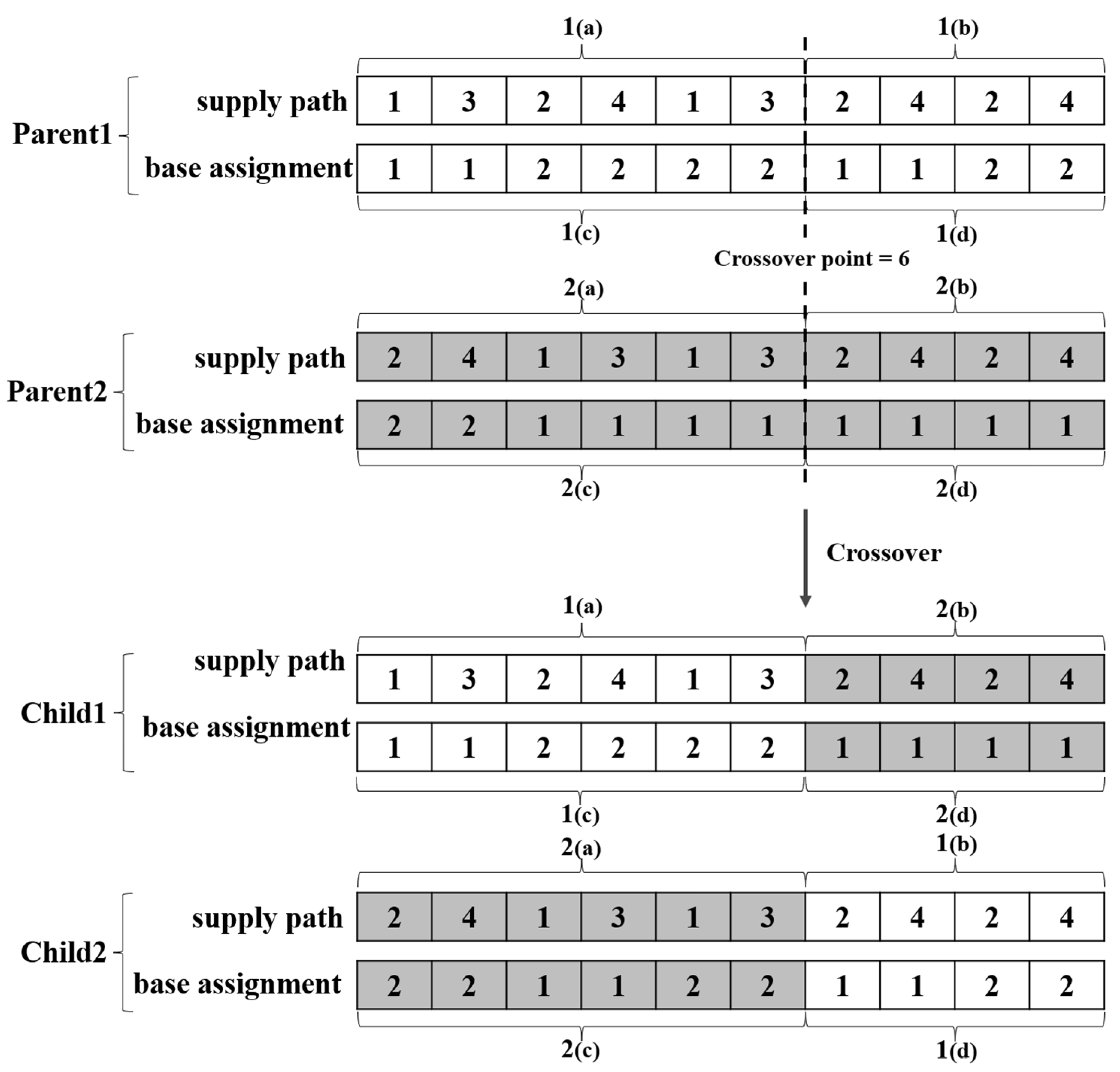
Next, a crossover operation is performed on each pair of selected parents. A crossover point is chosen randomly, ensuring it is at an even position within the individual’s length. For each parent, the sections before and after the crossover point are swapped to create two offspring. The path and base assignment parts of the individuals are crossed over separately. The problem context has been introduced in Section 4.1; an example of the crossover procedure is illustrated in Figure 3.
In Figure 3, Parent1 and Parent2 represent two selected individuals from the current population. According to the first row of parent1, {1, 3} indicates that the truck goes from harvest area f1 to plant p1, and {2, 4} indicates that the truck goes from harvest area f2 to plant p2, and so on. In this example, the crossover point is randomly selected at index 6, which falls within the path part. The genes before and after the crossover point are exchanged between Parent1 and Parent2 to produce two offspring, denoted as Child1 and Child2.
To introduce diversity, a mutation operation is applied to each offspring with a given mutation probability. In this mutation procedure:
  • The path part’s odd indices mutate to a random integer between 1 and F (representing a harvest area).
  • The path part’s even indices mutate to a random integer between F and F + P (representing a plant).
  • The base assignment part mutates to a random integer between 1 and B.
An example of the mutation procedure is illustrated in Figure 4. As shown in the Figure 4, two mutation points are randomly selected in the path part: index 1 mutates from 1 (representing harvest area f1) to 2 (f2), and index 6 mutates from 3 (plant p1) to 4 (p2). In the base assignment part, two pairs of mutation points are selected: the first pair, originally [2, 2] (base b2, b2), mutates to [1, 1] (base b1, b1); the second pair, originally [1, 1] (base b1, b1), mutates to [2, 2] (base b2, b2).
Since newly generated chromosomes may not always satisfy the initial supply and demand constraints, a repair operation is necessary. This repair operation works as follows:
  • Create deep copies of the initial supply and demand.
  • For each pair of indices in the path, check if the supply from the harvest area meets the demand from the plant for the required materials.
  • If a match is found, update the supply and demand accordingly and add the indices to the repaired path and base assignment.
  • If no match is found, randomly select new indices for the harvest area and plant until a match is found.
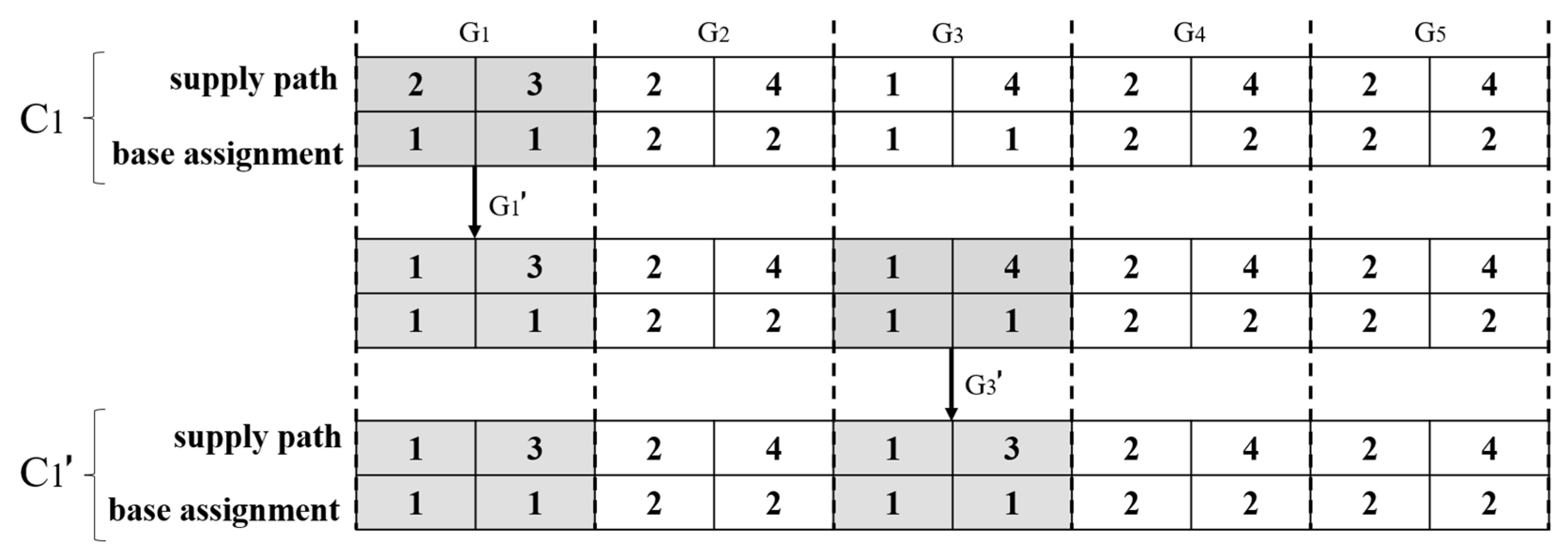
An example is illustrated in Figure 5. Suppose that a chromosome C1 is obtained after crossover mutation, traversing the path encoding part of the chromosome results in [2, 3, 2, 4, 1, 4, 1, 3, 2, 4]. According to the supply and demand relationships defined in Table 1, each gene is processed one by one. First, check {2, 3}: f2 does not contain m1, but p1 does. Since there are no matching materials, it enters the cycle of randomly selecting a new harvest area and plant, matching f1 and p1, and adds {1, 3} to the repaired path. Next, check {2, 4}: f2 contains m2 and p2 contains m2, satisfying the material matching condition, and it is directly added to the repaired path. Then, check the next gene {1, 4}, and so on.
These functions are combined to perform selection, crossover, mutation, and repair operations within the GA, generating new valid individuals for the next generation.

5. Numerical Experiments

In this section, numerical experiments are conducted to evaluate the performance of the developed GA. Initially, instances reported in [9] are adapted to clearly illustrate the advantage of the proposed GA in Section 5.1. Subsequently, sensitivity analysis on randomly generated instances is conducted in Section 5.2. All the numerical examples are coded in Python 3.10 Module Docs (64-bit) on a personal computer with an AMD Ryzen 7 5800H personal computer with 16 GB RAM.

5.1. Performance Evaluation on GA

To evaluate the performance of the proposed GA, we call it to solve the model presented in [9], and compare the final solutions with their results. Additionally, since the LNS algorithm proposed by Derigs et al. in [31] solves a similar model and demonstrates strong computational performance, we further compare the GA with both the commercial solver ILOG CPLEX version 12.7.1 linked in C++ environment and the LNS algorithm. The case study involves two groups of instances, i.e., Example I and Example II in [9] Specially, Example I considers a supply chain (SC) composed of 3 regional bases, 5 harvest areas, and 3 plants. Each base has 5 trucks available for hauling 30 full truckloads of 3 types of raw materials. Example II involves 5 regional bases, 10 harvest areas, and 3 plants. Each base has 10 trucks available for hauling 77 full truckloads of 2 types of raw materials.
The computational results are reported in Table 2. Columns 2 and 3 of Table 2 record the total cost and running time of Example I and Example II in [9]. Columns 4 and 5 record the objective value and the computation time (seconds) of the GA, while Columns 6 and 7 represent those of the LNS algorithm from [28].
T o t a l   c o s t   d e v i a t i o n ( % ) = | T o t a l   c o s t _ G A T o t a l   c o s t _ C | T o t a l   c o s t _ C .
According to Table 2, the developed GA demonstrates significant advantages in time efficiency, with negligible result errors. For Example I, ref. [9] optimally solved the model with the optimal cost of 35,005 USD in 16.86 CPU seconds. As a comparison, the developed GA solved the model in 1.28 CPU seconds, which is only 1.28 16.86 × 100 % = 7.5% of that in [9]. Additionally, the deviation of the GA solution to the optimum is only 1.26%. In contrast, the deviation of the LNS algorithm is slightly higher, at 2.04%. For Example II, CPLEX cannot output optimal solutions within 1800 s in [9]. While the developed GA output solutions in 2.56 s. As for the solution quality, the deviation of the GA solution is only 1.05% from the solutions obtained by CPLEX in [9]. The LNS algorithm took 3.21 CPU seconds, with a deviation of 2.81%. While the LNS algorithm showed reasonable results, the GA outperformed it by solving both examples faster and with lower cost deviations.
To ensure the statistical reliability of the results, each algorithm was executed 10 independent times in each instance, and a paired t-test was conducted to assess the significance of differences in total cost. According to Table 3, the results of the t-test indicate that the GA significantly outperforms the LNS algorithm in both instances, with p-values < 0.01, confirming the robustness and consistency of the proposed method.
Table 4 presents a comparison between the Genetic Algorithm (GA) and the Large Neighborhood Search (LNS) algorithm across different-scale cases. In Column 1 of Table 4, “b-f-p” represents different problem sizes, denoted as combinations of bases (b), harvesting areas (f), and plants (p). Across all cases, the GA consistently delivers lower total costs compared to the LNS algorithm. The primary reason for this discrepancy lies in the algorithm’s reliance on local search mechanisms, which can cause it to get trapped in local optima, particularly in large-scale instances with complex constraints. In contrast to the global search capability of GA, LNS explores the solution space more narrowly by incrementally adjusting the current solution, limiting its ability to escape suboptimal solutions. Furthermore, LNS is highly dependent on the initial solution; without a well-constructed starting solution, the algorithm’s performance may deteriorate significantly. While LNS is computationally more efficient in certain scenarios, this advantage diminishes when applied to problems that require extensive exploration of the solution space. Therefore, for complex, large-scale problems such as the Forest Logging Trucks Routing and Scheduling Problem (FRSP), the global search capability of GA makes it a more suitable choice for obtaining high-quality solutions in a shorter amount of time.

5.2. Sensitivity Analysis

In this section, we conduct a sensitivity analysis to identify the impact of the parameters on the FRSP. A total of 39 groups of large-scale instances, including different combinations of the number of bases and trucks, as well as various configurations of maximum work time and time windows, are tested. The computational results on sensitivity analysis are shown in Table 5.
The computational performance of the GA on large-scale randomly generated instances is shown in Table 5. Column 2 lists the runtime of the algorithm for different instances. To provide a clearer understanding, the results in Table 5 are presented in Figure 6.
As shown in Figure 6, the computation time of the GA exhibits a clear linear increase with the growth of problem size. Experimental results indicate that the algorithm consistently solves instances involving 5–25 regional bases, 10–50 harvest areas, and 5–10 plants within 30 s. This demonstrates that the algorithm is highly scalable, capable of efficiently handling increasingly large problem instances. It shows significant advantages in addressing large-scale FRSP problems and enables enterprises to achieve efficient and predictable optimization as their operations expand.
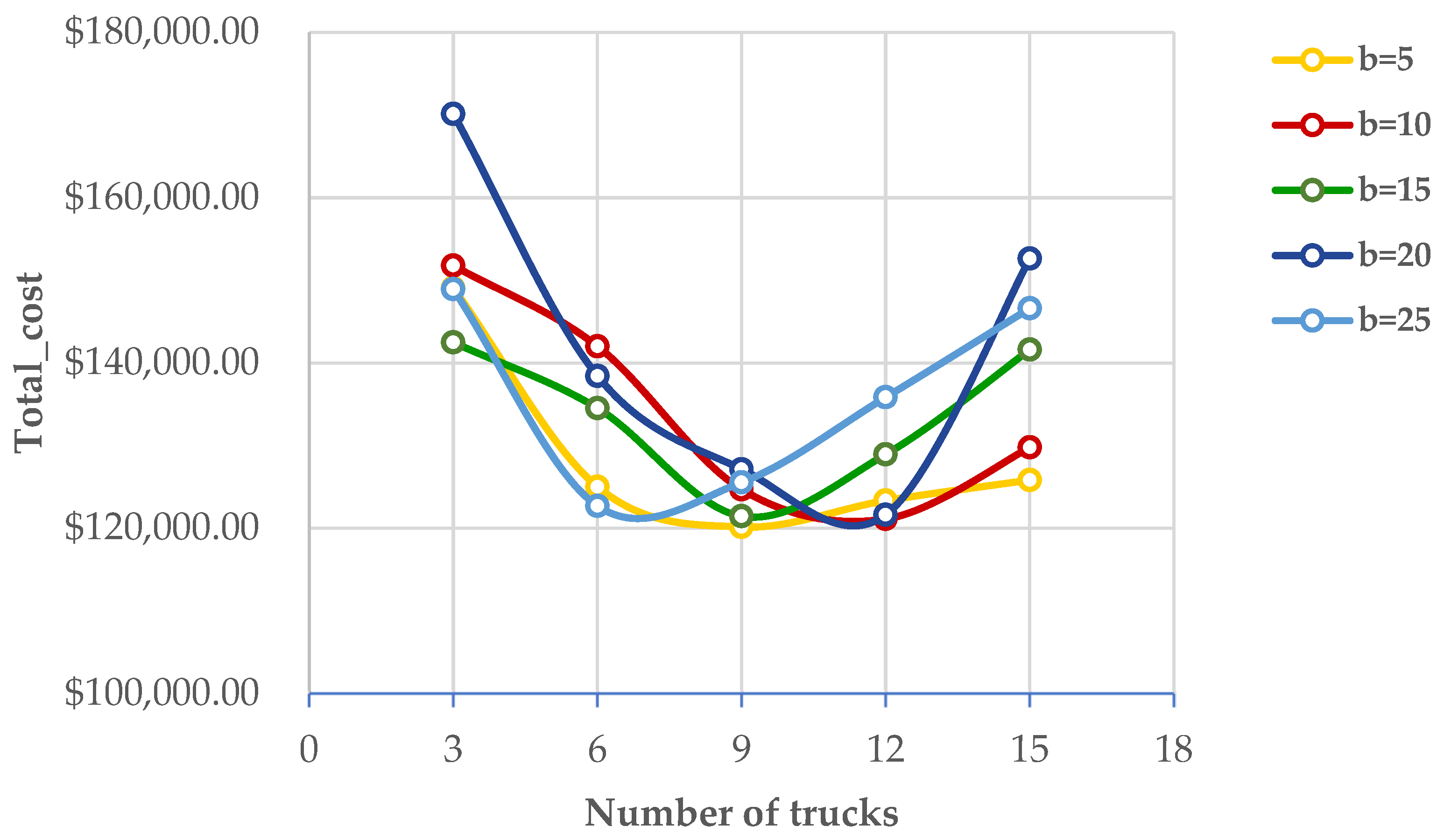
Table 6 shows the impact of different combinations of the number of bases (b) and the number of trucks (Nt) on the solutions for FRSP. Columns 1 of Table 6 shows the number of different bases. Columns 2 of Table 6 shows the number of different trucks. Columns 3 and 4 of Table 6 record the total cost and runtime of the GA solution, respectively. For a better understanding, the results in Table 6 are summarized in Figure 7.
As shown in Figure 7, each combination of base numbers and truck numbers exhibits an optimal point where the total cost is minimized. For example, when the number of bases is 5, or 15, the optimal number of trucks is approximately 9 (corresponding to the lowest point on the curve for each respective base number). When the number of bases is 20, the optimal number of trucks is 6. This indicates that for each configuration, there exists a specific combination of bases and trucks that can minimize the total cost as much as possible. Identifying the optimal combination of bases and trucks enables forestry companies to strategically allocate resources, minimizing costs and enhancing operational efficiency.
Table 7 shows the impact of maximum work time (Max_work_time) on the total cost (Total_cost). Column 1 of Table 7 shows the different work time limits. The total cost and computation time of the GA solutions under these varying time limits are recorded in Column 2 and Column 3, respectively. For better understanding, the results in Table 7 are summarized in Figure 8.
We can observe from Figure 8 that the total cost of GA solutions decreases as the maximum work time limit increases. The figure shows that extending the maximum work time from 6 h to 9 h has the most significant impact on reducing total cost, with a steep decline observed within this range. Beyond 9 h, the reduction in total cost becomes less pronounced, indicating a diminishing return on extending work time beyond this point. The analysis concludes that longer work hours allow for better resource utilization, as trucks can complete more deliveries within a single workday, thereby reducing the need for additional trips and associated costs. However, it is essential to balance worker fatigue and regulatory work hour limits. Companies can strategically allocate resources and schedule work shifts to align with the determined optimal work time.
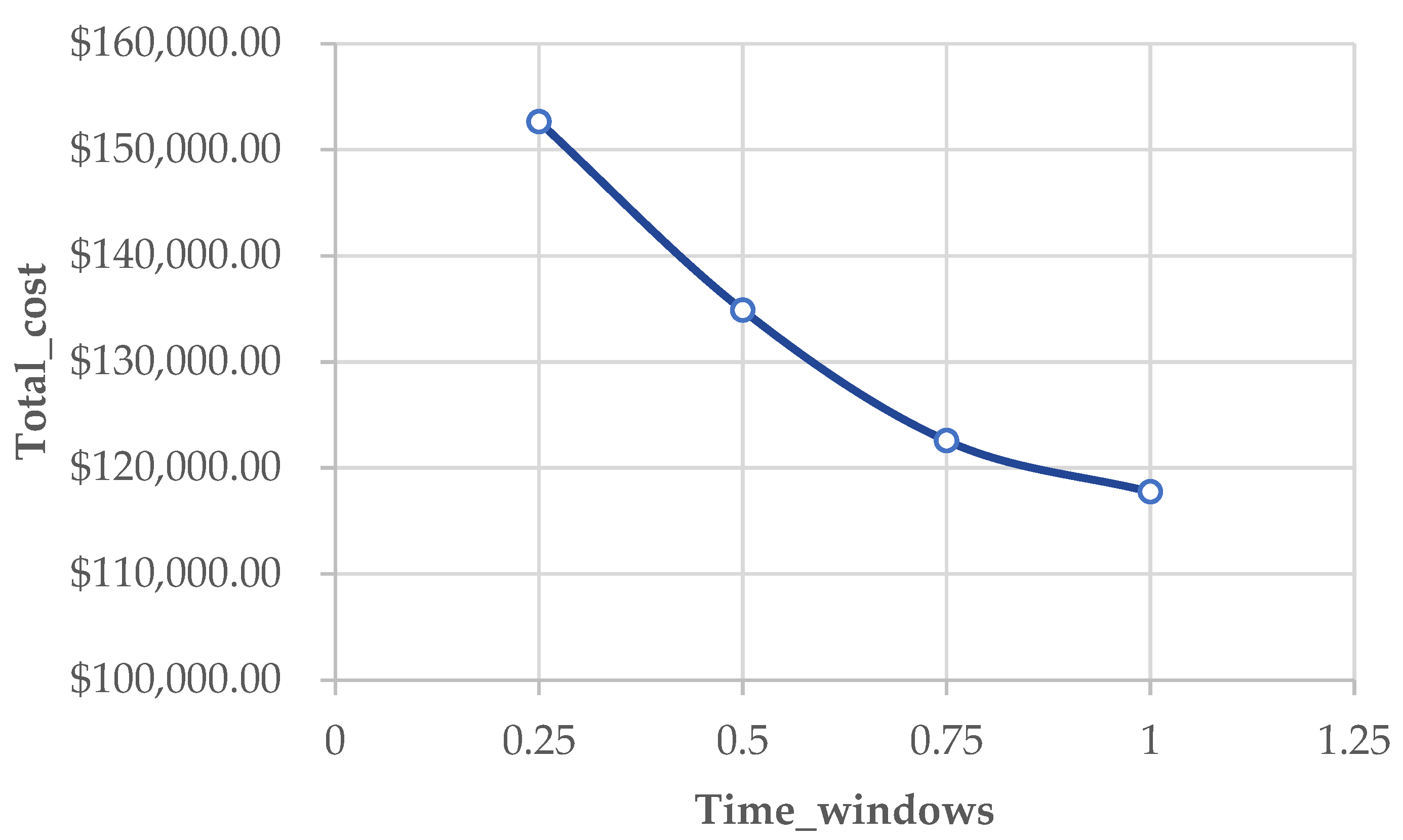
Table 8 shows the impact of the length of time windows (Time_windows) for receiving areas and processing plants on the total cost (Total_cost). Column 1 of Table 8 shows the different lengths of time windows. Column 2 and Column 3, respectively, record the total cost and computation time of the GA solutions under varying time windows. For better understanding, the results in Table 8 are summarized in Figure 9.
According to Figure 9, the total cost of GA solutions decreases as the length of time windows for receiving areas and processing plants increases. This result indicates that longer time windows allow for better coordination and flexibility in scheduling deliveries. Trucks have more time to complete deliveries, reducing the need for rush trips and associated costs. Companies can determine the optimal time windows based on real-world scenarios to minimize operational bottlenecks and achieve smoother logistics operations.
In summary, the sensitivity analysis indicates that the computation time of the GA increases linearly with the growth in problem size, making it a feasible alternative for large-scale problems. Additionally, optimizing the combination of bases and trucks, extending maximum work time, and increasing time windows are effective strategies for reducing total costs in forestry logistics. These adjustments can significantly enhance operational efficiency and resource utilization, making them crucial for companies aiming to minimize transportation costs and improve overall performance.

6. Conclusions

This study presents a novel GA heuristic to solve FRSP on large-scale instances. Specifically, the hybrid encoding method in the developed GA enhances its ability to represent the problem concisely. Furthermore, a decoding method is designed to find the optimal cost corresponding to the encoding. An efficient chromosome repair method is also developed to avoid infeasible solutions during the iterative process.
The results from the numerical experiments indicate that the proposed GA significantly reduces computation time while maintaining a high level of solution accuracy. In other words, the GA demonstrates considerable efficiency improvements over CPLEX, particularly in scenarios requiring rapid decision-making. This highlights the potential of the GA to be employed in real-world applications where timely and cost-effective solutions are critical.
Sensitivity analysis highlights that GA can efficiently handle the increasing complexity of larger-scale problems, making it a powerful tool for large-scale scenarios. By optimizing combination strategies and adjusting relevant parameters, companies can develop more efficient logistics plans that maintain cost-effective operations while meeting higher demands. This ensures that forestry logistics remain competitive and adaptable in a dynamic market environment.
Although classical graph algorithms (e.g., Dijkstra, A*) are often used in static shortest-path problems, they are not well-suited for FRSP due to its complex constraints such as time windows, truck reuse, depot coordination, and material-specific supply-demand matching. Instead, we compared the proposed GA with the LNS algorithm introduced by Derigs et al. [31], which was designed for a similar model and has demonstrated strong computational performance. This comparison, along with CPLEX, allows for a more realistic and fair assessment of GA’s performance under large-scale FRSP conditions. Future research may explore hybrid methods that combine graph-based preprocessing with evolutionary heuristics or spatially aware solution frameworks.
Despite the promising results, there are several avenues for future research to further enhance the performance and applicability of the proposed GA. One potential direction is to integrate other metaheuristic algorithms, such as Particle Swarm Optimization (PSO) or Ant Colony Optimization (ACO), to construct hybrid models that combine the strengths of multiple approaches. Additionally, future work could incorporate heterogeneous fleet structures, intermediate depots, or road accessibility constraints based on GIS data to better reflect real-world forestry operations. Refining the encoding and decoding mechanisms to improve scalability and adaptability across diverse problem settings is another valuable direction. Another important direction is to evaluate the robustness of the algorithm under conditions of data uncertainty and imperfection, which are common in real-world forestry logistics. In practice, supply information, vehicle availability, or travel times may be incomplete, noisy, or dynamically changing due to environmental and operational variability. Future research will incorporate stochastic modeling techniques and data perturbation scenarios to assess how the GA responds to such uncertainties and to further enhance its adaptability and real-world deployment potential.
In conclusion, the proposed GA provides a practical solution for FRSP, demonstrating significant potential for further development and application. By continuing to refine and expand upon this work, researchers can contribute to advancing optimization techniques and addressing complex logistical challenges in various domains.

Author Contributions

Conceptualization, W.D.; methodology, W.D.; software, X.F.; validation, X.F.; writing—original draft preparation, W.D.; writing—review and editing, X.F.; visualization, W.D.; supervision, X.F.; funding acquisition, X.F. All authors have read and agreed to the published version of the manuscript.

Funding

This work was supported by the Key Project of Philosophy and Social Science Research in Colleges and Universities in Jiangsu Province (No. 2023SJZD020). Thank you to the editors and anonymous reviewers for their kindly view and constructive suggestions.

Data Availability Statement

Data will be made available upon request.

Conflicts of Interest

The authors declare no competing interests.

Notations and Parameters

Sets
Bset of regional bases b.
Cset of available trucks c.
Cbset of trucks c that belongs to the regional base b.
Fset of harvest areas f.
Fmset of harvest areas f that offer raw material m.
Ifset of shifts i in f.
Lpset of shifts l in p.
Mset of raw materials m.
Pset of plants p.
Pmset of plants p that demand raw material m.
Δf,pset of pairs (i, l) with iIf and lLp such that l is allowed to be used after shift i.
Πp,fset of pair (i, l) with lLp and i ∈ If such that i is allowed to be used after shift l.
Ωb,fset of all shifts iIf that can be reached from b.
Vcset of loading capacity of vehicle C.
Parameters
CBFb,fcost (in USD per traveled kilometer) between nodes b and f.
CFPf,pcost (in USD per traveled kilometer) between nodes f and p.
CloseFfclosing time for harvest area f.
ClosePpclosing time for plant p.
CPBp,bcost (in USD per traveled kilometer) between nodes p and b.
CPFp,fcost (in USD per traveled kilometer) between nodes p and f.
DBFb,fdistance between nodes b and f.
DEMp,mdemand (in full truckloads) of material m at plant p.
DFPf,pdistance between nodes f and p.
DPBp,bdistance between nodes p and b.
DPFp,fdistance between nodes p and f.
EAWbmaximum ending time for truck departure from base b.
EFIf,iending time for a shift i of f.
EPLp,lending time for a shift l of p.
limNTnumber of allowed trips per truck.
Loadfloading time at harvest area f.
LRTctime limit for route performed by c.
OFf,msupply (in full truckloads) of material m at harvest area f.
OpeningFfopening time for harvest area f.
OpeningPpopening time for plant p.
SAWbminimum starting time for truck departure from base b.
SBFb,faverage speed to cross the path between nodes b and f.
SFIf,istarting time for a shift i of f.
SFPf,paverage speed to cross the path between nodes f and p.
SPBp,baverage speed to cross the path between nodes p and b.
SPFp,faverage speed to cross the path between nodes p and f.
SPLp,lstarting time for a shift l of p.
TBFb,frequired time to travel between nodes b and f.
TFPf,prequired time to travel between nodes f and p.
TPFp,frequired time to travel between nodes p and f.
TPBp,brequired time to travel between nodes p and b.
Unloadpunloading time at plant p.
WTFfmaximum waiting time for harvest area f.
WTPpmaximum waiting time for plant p.
Binary variables
xc,f,i,mtakes value 1 if the truck c departs from its regional base to the harvest area f for loading raw material m in shift i.
xc,f,i,p,l,mtakes value 1 if the truck c leaves the harvest area f at the end of shift i to unload raw material m at the plant p during shift l.
xc,p,l,f,i,mtakes value 1 if the truck c leaves the plant p at the end of shift l to load raw material m at the harvest area f during shift i.
xc,p,ltakes value 1 if the truck c leaves the plant p at the end of shift l and returns to its regional base.
Continuous variables
TCOSTtotal transportation costs.
TIMEc,btotal working time of truck c.

References

  1. Akay, A.O.; Demir, M. A Scenario-Based Analysis of Forest Product Transportation Using a Hybrid Fuzzy Multi-Criteria Decision-Making Method. Forests 2022, 13, 730. [Google Scholar] [CrossRef]
  2. Weintraub, A.; Navon, D. A Forest Management Planning Model Integrating Silvicultural and Transportation Activities. Manag. Sci. 1976, 22, 1299–1309. [Google Scholar] [CrossRef]
  3. Weintraub, A.; Barahona, F.; Epstein, R. A Column Generation Algorithm for Solving General Forest Planning Problems with Adjacency Constraints. For. Sci. 1994, 40, 142–161. [Google Scholar] [CrossRef]
  4. Weintraub, A.; Epstein, R.; Morales, R.; Seron, J.; Traverso, P. A truck scheduling system improves efficiency in the forest industries. Interfaces 1996, 26, 1–12. [Google Scholar] [CrossRef]
  5. Arthur, J.L.; Dykstra, D.P. Timber Harvest Planning—A Combined Optimization/Simulation Model. Environ. Manag. 1980, 4, 491–498. [Google Scholar] [CrossRef]
  6. Bordón, M.R.; Montagna, J.M.; Corsano, G. An exact mathematical formulation for the optimal log transportation. For. Policy Econ. 2018, 95, 115–122. [Google Scholar] [CrossRef]
  7. dos Santos, P.A.V.H.; da Silva, A.C.L.; Arce, J.E.; Augustynczik, A.L.D. A Mathematical Model for the Integrated Optimization of Harvest and Transport Scheduling of Forest Products. Forests 2019, 10, 1110. [Google Scholar] [CrossRef]
  8. Melchiori, L.; Nasini, G.; Montagna, J.M.; Corsano, G. Resources synchronization in a full truckload pickup and delivery problem: An exact approach. Comput. Oper. Res. 2023, 151, 106–118. [Google Scholar] [CrossRef]
  9. Melchiori, L.; Nasini, G.; Montagna, J.M.; Corsano, G. A mathematical modeling for simultaneous routing and scheduling of logging trucks in the forest supply chain. For. Policy Econ. 2022, 136, 102–693. [Google Scholar] [CrossRef]
  10. Schneeweiss, C. Distributed Decision Making; Springer Science & Business Media: Berlin/Heidelberg, Germany, 2012. [Google Scholar]
  11. Palmgren, M.; Rönnqvist, M.; Värbrand, P.; Palmgren, M.; Ro, M. A solution approach for log truck scheduling based on composite pricing and branch bound. Int. Trans. Oper. Res. 2003, 10, 15. [Google Scholar] [CrossRef]
  12. El Hachemi, N.; Gendreau, M.; Rousseau, L.M. A hybrid constraint programming approach to the log-truck scheduling problem. Ann. Oper. Res. 2011, 184, 163–178. [Google Scholar] [CrossRef]
  13. Vacca, I.; Salani, M.; Bierlaire, M. Optimization of Operations in Container Terminals: Hierarchical vs. Integrated Approaches. In Proceedings of the 10th Swiss Transport Research Conference, Ascona, Switzerland, 1–3 September 2010. [Google Scholar]
  14. Murphy, G. Reducing trucks on the road through optimal route scheduling and shared log transport services. South. J. Appl. For. 2003, 27, 198–205. [Google Scholar] [CrossRef]
  15. Malladi, K.T.; Sowlati, T. Optimization of operational level transportation planning in forestry: A review. Int. J. For. Eng. 2017, 28, 198–210. [Google Scholar] [CrossRef]
  16. Audy, J.F.; Rönnqvist, M.; D’Amours, S.; Yahiaoui, A.E. Planning methods and decision support systems in vehicle routing problems for timber transportation: A review. Int. J. For. Eng. 2023, 34, 143–167. [Google Scholar] [CrossRef]
  17. Gronalt, M.; Hirsch, P. Log-Truck scheduling with a tabu search strategy. Metaheuristics 2007, 39, 65–88. [Google Scholar]
  18. Flisberg, P.; Lidén, B.; Rönnqvist, M. A hybrid method based on linear programming and tabu search for routing of logging trucks. Comput. Oper. Res. 2009, 36, 1122–1144. [Google Scholar] [CrossRef]
  19. Haridass, K.; Valenzuela, J.; Yucekaya, A.D.; McDonald, T. Scheduling a log transport system using simulated annealing. Inf. Sci. 2014, 264, 302–316. [Google Scholar] [CrossRef]
  20. Iksan, N.; Tufail, A.; Apong, R.A.; Hidayatullah, A.F. Optimizing Maritime Passenger Transfer in Rich Vehicle Routing Problem Using a Hybrid Genetic Algorithm. IEEE Access 2024, 12, 80153–80164. [Google Scholar] [CrossRef]
  21. Bordón, M.R.; Montagna, J.M.; Corsano, G. Mixed integer linear programming approaches for solving the raw material allocation, routing and scheduling problems in the forest industry. Int. J. Ind. Eng. Comput. 2020, 11, 525–548. [Google Scholar] [CrossRef]
  22. Savuran, H.; Karakaya, M. Route optimization method for unmanned air vehicle launched from a carrier. Lect. Notes Softw. Eng. 2015, 3, 279–284. [Google Scholar] [CrossRef]
  23. Peng, K.; Du, J.; Lu, F.; Sun, Q.; Dong, Y.; Zhou, P.; Hu, M. A Hybrid Genetic Algorithm on Routing and Scheduling for Vehicle-Assisted Multi-Drone Parcel Delivery. IEEE Access 2019, 7, 49191–49200. [Google Scholar] [CrossRef]
  24. Moon, I.; Lee, S.; Bae, H. Genetic algorithms for job shop scheduling problems with alternative routings. Int. J. Prod. Res. 2008, 46, 2695–2705. [Google Scholar] [CrossRef]
  25. Baniamerian, A.; Bashiri, M.; Zabihi, F. Two phase genetic algorithm for vehicle routing and scheduling problem with cross-docking and time windows considering customer satisfaction. J. Ind. Eng. Int. 2018, 14, 15–30. [Google Scholar] [CrossRef]
  26. Cheikh, M.; Ratli, M.; Mkaouar, O.; Jarboui, B. A variable neighborhood search algorithm for the vehicle routing problem with multiple trips. Electron. Notes Discret. Math. 2015, 47, 277–284. [Google Scholar] [CrossRef]
  27. Cao, Q.; Fu, C.; Li, H. Route Planning for Chain Restaurants With Improved Delivery Mode Using an Adaptive Genetic Algorithm. IEEE Access 2022, 10, 25645–25656. [Google Scholar] [CrossRef]
  28. Maroof, A.; Ayvaz, B.; Naeem, K. Logistics Optimization Using Hybrid Genetic Algorithm (HGA): A Solution to the Vehicle Routing Problem with Time Windows (VRPTW). IEEE Access 2024, 12, 36974–36989. [Google Scholar] [CrossRef]
  29. Wang, Y.; Zhu, Q. A Hybrid Genetic Algorithm for Flexible Job Shop Scheduling Problem with Sequence-Dependent Setup Times and Job Lag Times. IEEE Access 2021, 9, 104864–104873. [Google Scholar] [CrossRef]
  30. Holland, J.H. Adaptation in Natural and Artificial Systems; University of Michigan Press: Ann Arbor, MI, USA, 1975. [Google Scholar]
  31. Derigs, U.; Pullmann, M.; Vogel, U.; Oberscheider, M.; Gronalt, M.; Hirsch, P. Multilevel Neighborhood Search for Solving Full Truckload Routing Problems Arising in Timber Transportation. Electron. Notes Discret. Math. 2012, 39, 281–288. [Google Scholar] [CrossRef]
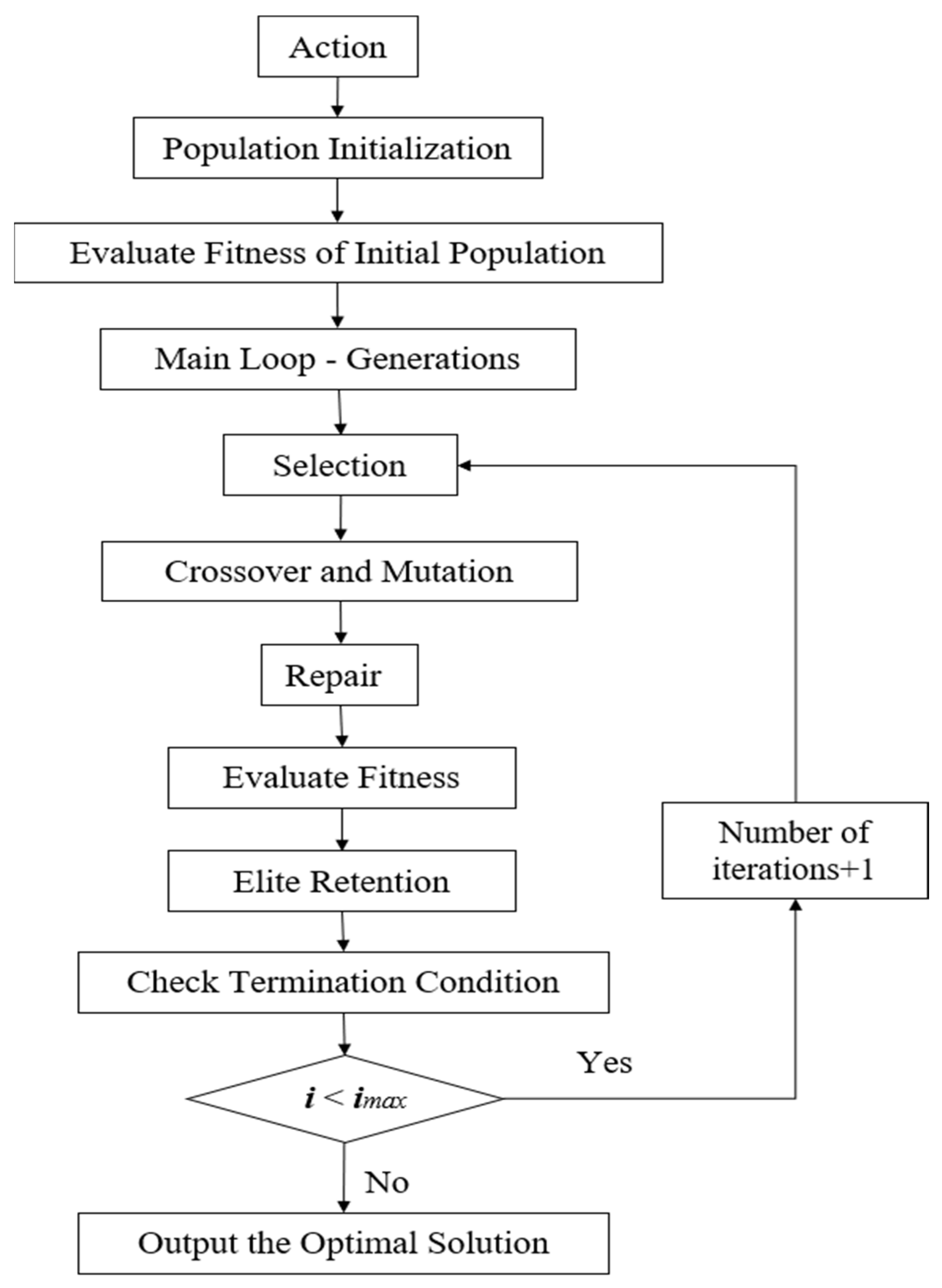
Figure 1. The framework of GA.
Forests 16 01440 g001
Figure 2. Example of the encoding representation.
Forests 16 01440 g002
Figure 3. Example of the crossover operator.
Forests 16 01440 g003
Figure 4. Example of the mutation operator.
Forests 16 01440 g004
Figure 5. Example of the repairing operator.
Forests 16 01440 g005
Figure 6. The trend of GA runtime increase.
Forests 16 01440 g006
Figure 7. The trends observed in different combinations.
Forests 16 01440 g007
Figure 8. The trend of total costs under different time constraints.
Forests 16 01440 g008
Figure 9. The trend of total costs under different lengths of time windows.
Forests 16 01440 g009
Table 1. Information in the numerical example.
b1b2f1f2m1m2
b1--4532--
b2--1070--
p19932148220
p21067365403
m1--23--
m2--00--
Table 2. The computational results.
Total
Cost_C
CPU_CTotal
Cost_GA
CPU_GATotal Cost
Deviation
(%)
Total
Cost_LNS
CPU_LNSTotal Cost
Deviation
(%)
I35,005 USD16.8635,445 USD1.281.2635,720 USD1.672.04
II117,890 USD1800119,130 USD2.561.05121,670 USD2.813.21
Table 3. GA and LNS comparison over 10 independent runs.
RunTotal Cost_GATotal Cost_LNS
135,445 USD35,720 USD
235,445 USD35,720 USD
335,445 USD35,815 USD
435,560 USD35,900 USD
535,600 USD35,900 USD
635,615 USD35,980 USD
735,650 USD36,005 USD
835,650 USD36,010 USD
935,720 USD36,055 USD
1035,815 USD36,140 USD
Table 4. GA and LNS comparison in large-scale cases.
b-f-pTotal Cost_GATotal Cost_LNS
5-10-5118,825 USD121,055 USD
10-20-10304,425 USD336,980 USD
15-30-15457,815 USD462,405 USD
20-40-20588,505 USD622,630 USD
25-50-25736,370 USD778,115 USD
Table 5. Experiments on the randomly generated instances.
b-f-pCPU_GA(s)
5-10-51.3682
10-20-104.0425
15-30-158.0023
20-40-2014.4467
25-50-2522.0584
Table 6. Experiment for instances.
bNtTotal Cost (USD)CPU_GA (s)
3149,0850.8737
6125,0151.3085
59120,1702.0508
12123,3502.0311
15125,8302.0542
3151,7800.8647
6140,1351.2247
109124,7252.0696
12121,1202.0234
15129,8052.0516
3142,4950.9114
6134,5401.1626
159121,4752.1132
12128,9352.1276
15141,6202.1317
3170,1500.9375
6138,4301.3014
209127,1552.0961
12121,6352.1435
15152,6352.0215
3148,9250.8550
6122,7051.3018
259125,5652.0524
12135,8552.0816
15146,6352.1168
Table 7. Sensitivity analysis of Max_work_time.
Max_Work_Time (h)Total Cost (USD)CPU_GA (s)
3-2.3488
6154,8702.2032
9122,5702.0639
12117,7552.1402
15116,3152.1679
Table 8. Sensitive analysis of Time_windows.
Time_Windows (h)Total Cost (USD)CPU_GA (s)
0.25152,6502.5427
0.5134,8702.2146
0.75122,5702.3577
1117,7552.1497
Disclaimer/Publisher’s Note: The statements, opinions and data contained in all publications are solely those of the individual author(s) and contributor(s) and not of MDPI and/or the editor(s). MDPI and/or the editor(s) disclaim responsibility for any injury to people or property resulting from any ideas, methods, instructions or products referred to in the content.