Article

Modeling Urban-Vegetation Aboveground Carbon by Integrating Spectral–Textural Features with Tree Height and Canopy Cover Ratio Using Machine Learning

School of Architecture, Southeast University, Nanjing 210096, China
*
Author to whom correspondence should be addressed.
Forests 2025, 16(9), 1381; https://doi.org/10.3390/f16091381
Submission received: 23 July 2025 / Revised: 20 August 2025 / Accepted: 26 August 2025 / Published: 28 August 2025
(This article belongs to the Section Urban Forestry)

Abstract

Accurately estimating aboveground carbon storage (AGC) of urban vegetation remains a major challenge, due to the heterogeneity and vertical complexity of urban environments, where traditional forest-based remote sensing models often perform poorly. This study integrates multimodal remote sensing data and incorporates two three-dimensional structural features—mean tree height ( H m e a n ) and canopy cover ratio (CCR)—in addition to conventional spectral and textural variables. To minimize redundancy, the Boruta algorithm was applied for feature selection, and four machine learning models (SVR, RF, XGBoost, and CatBoost) were evaluated. Results demonstrate that under multimodal data fusion, three-dimensional features emerge as the dominant predictors, with XGBoost using Boruta-selected variables achieving the highest accuracy (R2 = 0.701, RMSE = 0.894 tC/400 m2). Spatial mapping of AGC revealed a “high-aggregation, low-dispersion” pattern, with the model performing best in large, continuous green spaces, while accuracy declined in fragmented or small-scale vegetation patches. Overall, this study highlights the potential of machine learning with multi-source variable inputs for fine-scale urban AGC estimation, emphasizes the importance of three-dimensional vegetation indicators, and provides practical insights for urban carbon assessment and green infrastructure planning.

1. Introduction

1.1. The Value and Complexity of Estimating Urban-Vegetation Aboveground Carbon Storage (AGC)

Urban vegetation, as a critical component of green infrastructure, plays an essential role in mitigating climate change, improving ecosystem services, and enhancing residents’ quality of life [1,2,3]. Accurately quantifying its AGC is crucial for urban ecological planning, resource allocation, and achieving carbon neutrality goals [4,5]. However, estimating AGC in urban areas remains challenging. due to the high heterogeneity of vegetation types, community structures, and human disturbances [6,7]. Unlike natural forests, urban vegetation exhibits complex horizontal patterns (e.g., mixed plantations and monoculture patches) and vertical stratifications (e.g., grasslands, shrub layers, multi-layered tree communities), both of which significantly influence carbon stock [8]. These complexities, coupled with environmental disturbances such as air pollution and soil degradation, reduce the transferability and precision of traditional forest-based models when applied to urban settings [9].

1.2. Progress and Limitations of Estimating Urban-Vegetation ACG by Remote Sensing (RS)

1.2.1. Traditional RS Estimation

Remote sensing methods have been widely adopted to estimate urban AGC, primarily using either area-based coefficient models (e.g., InVEST) [10,11] or statistical regression models based on spectral indices [12,13,14]. While the former offer simplicity, they lack adaptability and spatial specificity. The latter improve accuracy but often rely solely on 2D spectral and textural information, which fails to capture sub-canopy structures critical for biomass estimation [15,16]. Traditional vegetation indices such as NDVI, RVI, and EVI reflect “greenness” as a proxy for potential photosynthetic activity [17], and are therefore widely applied in AGC estimation, due to their relatively good correlation with biomass [18]. However, estimation accuracy based on these indices still shows significant regional variability (R2 = 0.45–0.85) [19,20]. The heterogeneous distribution of urban vegetation further exacerbates uncertainties, as mixed pixels strongly affect carbon storage assessments. In addition, the unique structural and functional characteristics of urban vegetation (UV) result in carbon sequestration processes that differ substantially from those of natural ecosystems. Consequently, conventional RS-based methods continue to face considerable challenges in improving the predictive accuracy of urban AGC.

1.2.2. Multimodal RS Estimation

The development of multimodal remote sensing (RS) technologies, including multispectral, hyperspectral, and LiDAR data, has created new opportunities for accurately estimating urban-vegetation AGC [21,22]. Integrating or jointly utilizing cross-modal datasets has proven promising in overcoming the limitations of single-source data, thereby providing a more comprehensive representation of vegetation carbon storage capacity [23,24]. Recent advancements in LiDAR and high-resolution satellite imagery have substantially improved the ability to characterize both vertical and horizontal vegetation structures in urban green spaces [23,25]. Large-scale missions such as GEDI and ICESat-2 have made it possible to acquire three-dimensional (3D) surface data at unprecedented spatial extents [23].
Nevertheless, extracting urban-vegetation information through the integration of multi-source optical imagery remains challenging [26]. LiDAR provides precise measurements of tree height (H) [27], while high-resolution imagery enables accurate derivation of canopy cover ratio (CCR) [28]. Both parameters—canopy height and canopy cover—are critical for reducing uncertainties in carbon storage modeling [29,30], as they jointly reflect aboveground biomass (AGB) distribution [31,32]. Importantly, these structural attributes capture vegetation heterogeneity that cannot be fully represented by spectral or textural features alone. Thus, incorporating H and CCR into AGC modeling enhances structural sensitivity and significantly improves predictive accuracy in complex urban environments. However, it is still a challenge to accurately retrieve canopy height and other key structural parameters from remote sensing [33], especially when using them to estimate urban-vegetation AGC [23,34].

1.2.3. Advanced Algorithm Model

Carbon storage estimation involves both model-related and measurement-related uncertainties, with model uncertainty accounting for approximately 70% of the total [35]. Numerous studies have investigated the estimation of urban forest carbon storage using remote sensing approaches [36]. Conventional multiple linear regression (MLR) models offer certain advantages in predicting forest biomass [37]; however, they are insufficient to fully capture the complex and nonlinear relationships between independent variables and AGC.
In recent years, the emergence of machine learning algorithms such as support vector regression (SVR), random forest (RF), deep learning (DL), and ensemble learning (EL) has significantly improved the accuracy of forest AGC estimation [38,39], providing more robust alternatives to traditional regression models [40]. Among these, boosting algorithms—also referred to as enhancement or boosting methods—have gained particular attention, as they enhance predictive accuracy by transforming weak learners into strong learners [41]. Within this family, Extreme Gradient Boosting (XGBoost version 3.0.4) and Categorical Boosting (CatBoost version 1.2.8) are widely recognized as state-of-the-art techniques, especially effective when training sample sizes are relatively small [42]. Previous studies have reported improved performance of forest AGC estimation using these methods [43], particularly when integrating multi-source datasets [44].
Nonetheless, it is important to critically assess the applicability and generalizability of these algorithms across different ecological and spatial contexts [45]. Moreover, balancing model accuracy with computational efficiency remains a key consideration [46], highlighting the necessity of selecting optimal variable subsets when using multi-source RS data, in order to reduce both data dimensionality and computational complexity [47].

1.3. Objectives and Innovations of This Study

This study has three key contributions. Firstly, we try to introduce multi-source remote sensing data into the AGC modeling of urban vegetation; that is, two three-dimensional variables, tree height and canopy coverage. This approach extends the traditional spectral texture framework. Although previous studies have applied canopy height or CCR to biomass estimation in general vegetation or forest environments, its application in AGC modeling of urban green space is still limited and not fully explored [48]. Secondly, the ability of machine learning to estimate the aboveground carbon storage of urban vegetation under multi-source variable input is used and evaluated, and combined with the SHAP analysis, the relative importance of all input characteristics is quantified. This initiative explores the value of models and variables in terms of accuracy and interpretability. Third, taking Nanjing as an example, the prediction effectiveness under different green space types is compared, which provides practical enlightenment for targeted urban carbon management.

2. Data and Methods

This study integrated multi-source data and on-site measurements to construct and validate a framework for estimating urban green space carbon storage using three-dimensional variables. The workflow consists of five parts, including (1) data acquisition, (2) data processing, (3) model training, (4) model evaluation and feature analysis, and (5) carbon stock prediction and validation (Figure 1).

2.1. Data Acquisition

2.1.1. Study Area and Sampling Strategy

This study was conducted in five main districts located south of the Yangtze River in Nanjing, a city situated in the mid-latitude subtropical zone between the central and northern subtropics. The region is dominated by mixed evergreen and deciduous broadleaf forests. With 117 rainy days on average per year and 1294.4 mm of rainfall, the average annual temperature is 17.1 °C [49].
Due to the pronounced spatial heterogeneity and vertical complexity of urban vegetation, full-coverage sampling is often infeasible [50]. Therefore, the research adopted a stratified sampling approach to capture variability in vegetation structure and carbon storage by selecting representative green space types and plant community compositions [17].
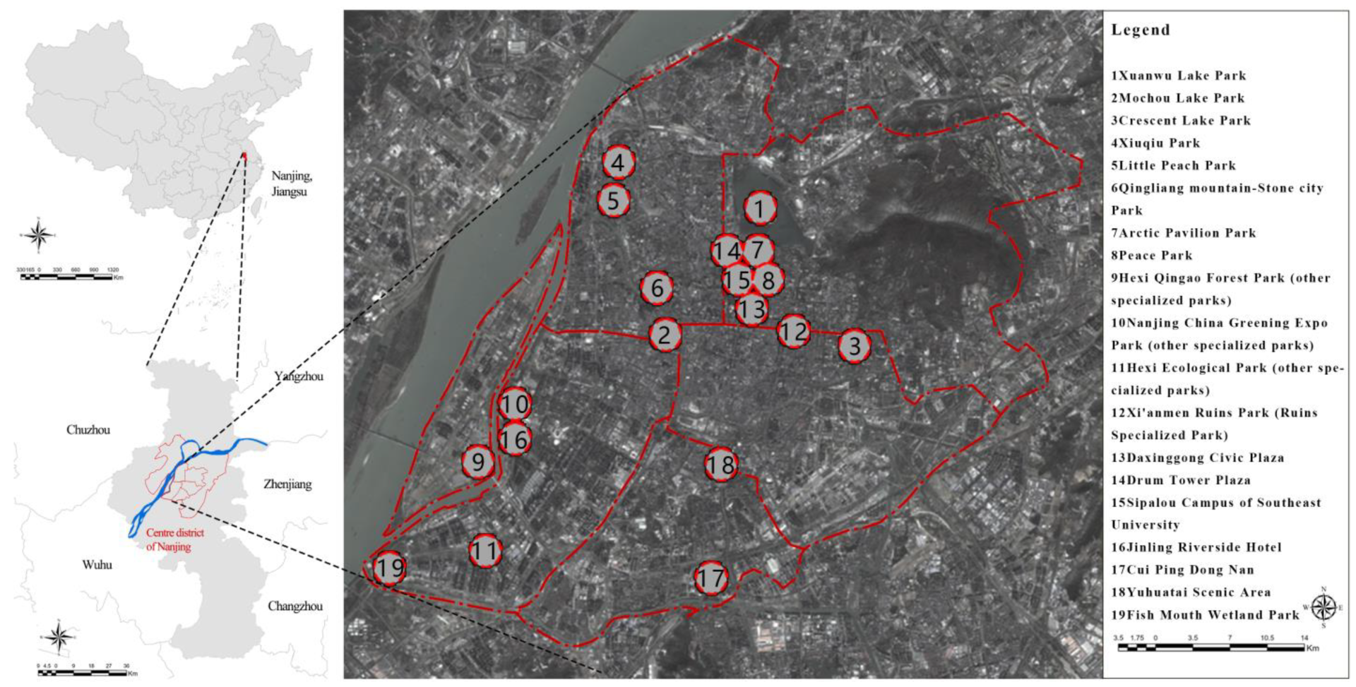
Sampling plots measuring 20 m × 20 m were established for each plant community. The sample plots are distributed as evenly as possible in each green space, and the number of sample plots was weighted, based on the total area of each green space type, to ensure at least 10% spatial coverage. Based on this approach, 19 representative green spaces were selected across the five districts, comprising a total of 408 plant community plots. Community types were categorized and abbreviated, based on field survey results. In this study, the sampling design followed recommendations from previous urban forest surveys, which suggest a minimum of approximately 200 plots, with most studies rarely exceeding 500 [51]. Accordingly, 408 circular plots (0.04 ha each) exceeded the minimum threshold and remained within the generally accepted range.
The spatial distribution of the study area and sampling plots is shown in Figure 2. A summary of sampling sites and plot numbers is provided in Appendix A Table A1, and community classifications are listed in Table A2.
All trees in each plot were visually identified to species level by professionally trained master’s degree candidates. To efficiently obtain tree structural parameters (diameter at breast height, height, and crown width), we scanned the plots using the OSlam RTK-SLAM-R6 backpack LiDAR system, which provides 3D point clouds with 2–4 cm accuracy. Data were collected in two seasonal phases (winter: January–February 2024; summer: June–July 2024) between 8:00–12:00 and 14:00–18:00 daily.
For quality control, we randomly selected 20% of the trees in each plot and con-ducted manual measurements using a diameter tape measure and a laser rangefinder. These measurements were cross-validated with the data obtained from the LiDAR, achieving an overall accuracy rate of 93.7%. Then, based on the identified tree species, we applied specific allometric equations. Also, cross-validation was performed between the winter and summer datasets, with the summer survey used in cases of inconsistencies.
Each community was treated as an independent unit, labeled as “plot-community ID.” The southwest corner of each plot was geolocated using GPS, and plot boundaries were delineated using compass bearings and tape measurements (closure error < 1/200, where closure error refers to the positional difference between the start and end points after measuring a closed loop, expressed as a proportion of the total measured distance).

2.1.2. Remote Sensing Data

Sentinel-2 Level-2A multispectral imagery was used in this study, which is geometrically, radiometrically, and atmospherically corrected. Data were downloaded from the Copernicus Open Access Hub (https://dataspace.copernicus.eu/ (accessed on 10 January 2025)). The sensor provides 13 spectral bands (400–2400 nm) at spatial resolutions of 10–60 m, enabling effective extraction of urban-vegetation characteristics. To capture peak vegetation conditions, imagery acquired on 5 July 2024 was selected for spectral analysis. All vegetation indices in this study were calculated using 10 m resolution Sentinel-2 bands (B2, B3, B4, B8), and texture features were derived from NDVI to ensure a consistent spectral source. To match the 20 m × 20 m field plot scale, all Sentinel-2-derived layers, including spectral, index, and texture features, were resampled to 20 m resolution, using bilinear interpolation.

2.1.3. Data from the Literature

In addition to field investigations and remote sensing products, the parameters for calculating carbon storage rely partly on published literature. Specifically, the aboveground carbon (AGC) of each tree is calculated using the biomass conversion method, which requires a species-specific allometric growth equation and carbon content coefficient. When specific parameters for Nanjing were unavailable, values were compiled from peer-reviewed studies conducted in Eastern China, where similar climatic and ecological conditions prevail (see details in Table A3 for allometric equations and Table A4 for carbon content factors).

2.2. Data Processing

2.2.1. H m e a n and CCR of Sample Plots

To characterize the three-dimensional vegetation structure within each plot, two indicators were calculated: the mean tree height ( H m e a n ) and the canopy cover ratio (CCR). Together, these two metrics capture complementary aspects of stand structure, linking canopy morphology with biomass accumulation potential. H m e a n represents the average height of all individual trees in a plot, serving as a proxy for vertical biomass distribution. CCR is defined as the ratio of total canopy area to plot area, reflecting horizontal vegetation density and spatial occupancy. Specifically, individual tree height and crown area were extracted from LiDAR point clouds using single-tree segmentation. H m e a n was then computed as the sum of all tree heights divided by the number of trees within the plot (Equation (1)).
H m e a n = i = 0 n H i n
where
H m e a n : The average tree height of the sample plot (m);
H i : The height of the i-th tree in the sample plot (m);
n : The total number of trees in the sample plot.
CCR was obtained by dividing the aggregated crown projection area of all trees by the total plot area (Equation (2)).
C C R = i = 0 n C A i A
where
C C R : Tree canopy cover ratio of the sample plot (%);
C A i : Crown area of the i-th tree (m2);
A : Sample area (m2).

2.2.2. AGC for Single Trees and Sample Plots

(1)
Biomass estimation
Biomass (B) was calculated from LiDAR-derived diameter at breast height (DBH) and height (H), using allometric equations. This equation usually has two basic forms, based on the principle of obtaining the biomass of a certain organ of a tree through breast height diameter and tree height (Equations (3) and (4)):
B i j = a D b
Or   B i j = a D 2 H b
where
B i j : Biomass of organ j of tree species i in kilograms (kg) (usually includes trunk, branches, leaves and bark);
D: Diameter at breast height in centimeters (cm);
H: Tree height in meters (m);
a, b: Fitting coefficients.
Furthermore, the aboveground biomass (AGB) is obtained by summarizing the biomass of each part. (Some trees can also directly obtain AGB through the biomass equation in the above form.) AGB of tree species is calculated in Equation (5):
A G B = B t + B b r + B l e + B b a
where
A G B : Aboveground biomass of tree species i in kilograms (kg);
B t : Trunk biomass in kilograms (kg);
B b r : Branch biomass in kilograms (kg);
B l : Leaf biomass in kilograms (kg);
B b a : Bark biomass in kilograms (kg).
(2)
AGC estimation
AGC was derived by AGB using species-specific carbon content (CF), as in Equation (6).
A G C = A G B × C F
where AGC is the aboveground carbon (kgC); A G B is the aboveground biomass (kgC); and CF is the carbon content rate.

2.2.3. Remote Sensing Feature Extraction

(1)
Spectral and Texture Features
Spectral features included twelve Sentinel-2 bands and four vegetation indices commonly associated with carbon estimation: DVI, NDVI, EVI, and RVI [52,53].
Texture features were derived from the NDVI layer using gray-level co-occurrence matrix (GLCM) metrics [54]: Mean, Variance, Correlation, Contrast, Entropy, Homogeneity, Dissimilarity, and Second Moment. These were calculated at five window sizes (3 × 3, 5 × 5, 7 × 7, 9 × 9, 11 × 11), yielding 40 texture features in total. Prior to GLCM computation, the input image was quantized into 64 gray levels, in accordance with the default configuration of ENVI software (version 5.3).
This quantization level has been widely adopted in remote sensing texture analysis, as it provides a suitable compromise between preserving meaningful texture information and ensuring computational efficiency [55,56]. Moreover, excessively high quantization levels (e.g., 256 gray levels) can lead to sparse co-occurrence matrices, which may undermine the accuracy of probability estimation and, in turn, affect the reliability of texture metrics [57]. Hence, the choice of 64 gray levels ensures both computational stability and efficiency.
(2)
Tree height and Canopy cover ratio data for prediction
(a)
Tree height (H)
The canopy height model employed in this study was developed by EcoVision Lab at ETH Zurich [58] and originally trained on GEDI data up to 2020. For this research, we applied the model to Sentinel-2 imagery acquired in 2024, to estimate contemporary canopy height. Although the model has not been retrained with ground-truth data from 2024, it utilizes spectral and structural information from the current imagery, enabling estimation of up-to-date canopy heights. Nevertheless, potential uncertainties may arise due to vegetation growth dynamics or structural changes occurring after the model’s training period. This temporal mismatch should be considered when interpreting the results, and future work could include validation with field-measured data or updated model training to improve accuracy.
  • (b)
    Canopy cover ratio (CCR)
The CCR was derived through a multi-resolution workflow designed to enhance spatial accuracy. First, urban green space boundaries were extracted from a 1 m resolution dataset developed by UGSNet at Sun Yat-sen University [59], with an overall accuracy of 87.56%. Within these green space areas, tree crowns were delineated as regions with canopy height ≥ 3 m, based on tree height data. These crown areas were then aggregated to 10 m grid cells, within which the crown-covered area was calculated. Finally, to match the 20 m spatial resolution of field plots and other model variables, all CCR values were resampled to 20 m, using average aggregation. The CCR for each 20 m cell was thus defined as the proportion of tree crown area to total green space area within the cell, capturing the horizontal canopy density while excluding low vegetation layers.
In total, 58 variables were extracted, including spectral, textural, and 3D structural features (Table A5), to model their relationships with plot-level AGC.

2.2.4. Data Alignment and Consistency Analysis

To ensure data consistency across sources, all variables—including LiDAR-derived 3D features, spectral indices, and texture metrics—were spatially aligned to the same coordinate system (WGS 84) and resampled to 20 m resolution. Prior to model input, all continuous variables were standardized using z-score normalization, to eliminate scale differences and enhance model convergence and comparability.
To evaluate the consistency between the airborne LiDAR-derived H m e a n and CCR used in model training and the GEDI- and UGSNet-based 3D features used for mapping, we conducted a consistency assessment using Pearson correlation (r), root mean square error (RMSE), and bias. The results showed strong agreement for both variables, with H m e a n exhibiting a high correlation (r = 0.882), an RMSE of 2.586 m, and a bias of −1.012 m, indicating a slight underestimation in GEDI-derived heights. Similarly, CCR showed good consistency (r = 0.813), with minimal RMSE (0.175) and negligible bias (0.002), confirming the reliability of the mapping data inputs.

2.2.5. Sample Separation Before Training

A total of 408 ground samples were collected for model development. To ensure a balanced evaluation of model performance, the dataset was randomly partitioned into three subsets: 70% (286 samples) for model training, 20% (82 samples) for testing, and the remaining 10% (40 samples) reserved as an independent validation set. The training and testing subsets were used iteratively for model fitting and performance optimization, while the independent validation set was withheld throughout the modeling process. This separation strategy was adopted to minimize overfitting and to provide a rigorous assessment of the model’s generalization ability under practical application scenarios.

2.3. Model Training

2.3.1. Feature-Variable Screening

Effective feature selection is critical for improving model performance in AGC estimation [60]. This study employed the Boruta algorithm to identify the most relevant predictors from the initial feature set. Boruta iteratively compares the importance of each variable with that of randomized shadow features, retaining only those with significantly higher importance [61]. This reduces redundancy, enhances model generalizability, and minimizes overfitting. To evaluate the contribution of 3D structural features, models were trained using four variable sets: all features, spectral only, spectral + texture, and Boruta-selected features. The model with the highest accuracy was selected for further analysis.

2.3.2. Four Machine Learning Algorithms

To capture complex, nonlinear relationships in urban-vegetation AGC estimation, four proven machine learning models were selected: SVR, RF, XGBoost, and CatBoost.
SVR excels at modeling nonlinear trends in moderate-size, low-noise data by mapping features into high-dimensional space [62]. RF is robust to noise and overfitting, with strong interpretability and minimal tuning needs [63]. XGBoost improves accuracy and speed through regularization and parallel processing, effectively handling missing data and multicollinearity [64]. CatBoost further reduces overfitting via ordered boosting, and handles complex, noisy data well [65].
These four models were selected not only for their high performance across remote sensing applications, but also for their complementary strengths: SVR for its robustness in low-noise settings, RF for interpretability and resistance to overfitting, XGBoost for efficiency and accuracy, and CatBoost for its superior handling of complex interactions and feature distributions. By leveraging their diverse advantages, we systematically compared them, to identify the best fit for AGC modeling.

2.4. Evaluation and Feature Analysis

2.4.1. Model Accuracy Test

Model performance was evaluated using the coefficient of determination (R2), root mean square error (RMSE), and relative root mean square error (RRMSE), which are standard metrics for regression accuracy [66]. Higher R2 values (closer to 1) indicate better model fit, while lower RMSE and RRMSE reflect smaller prediction errors. The calculation formulas are provided in Equations (7)–(9).
  R M S E = 1 n i = 1 n y i y i ^ 2
  R R M S E = R M S E y i ¯ × 100 %
R 2 = i = 1 n y i ^ y i ¯ 2 i = 1 n y i y i ¯ 2
where y i is the actual sample measurement; y i ¯ is the sample mean; y i ^ is based on the predicted values obtained from the model; and n is the sample size.

2.4.2. Shapley Additivity (SHAP)

For the highest-performing models, interpretability was assessed using the SHAP method. Grounded in cooperative game theory, SHAP quantifies the individual contribution of each input feature to the model’s output, including feature interactions [67]. The SHAP summary plot provides a global overview of feature importance and the direction of their effects, while dependency plots offer detailed insights into the relationship between specific feature values and their contributions, elucidating the internal mechanisms of the model.

2.5. Prediction and Validation

The best-performing model identified through training and evaluation was subsequently applied to predict the aboveground carbon storage across the central urban area of Nanjing. Model inputs consisted of spectral, textural, and three-dimensional structural metrics derived from remote sensing data, with the specific variables determined according to the selected model. To assess the reliability and robustness of the prediction results, an independent validation dataset comprising 40 field plots, which had been set aside prior to model training, was employed. The predicted values were compared with field-based estimates to evaluate model performance and ensure the credibility of large-scale carbon storage mapping.

3. Results

3.1. Feature Importance and Relevance

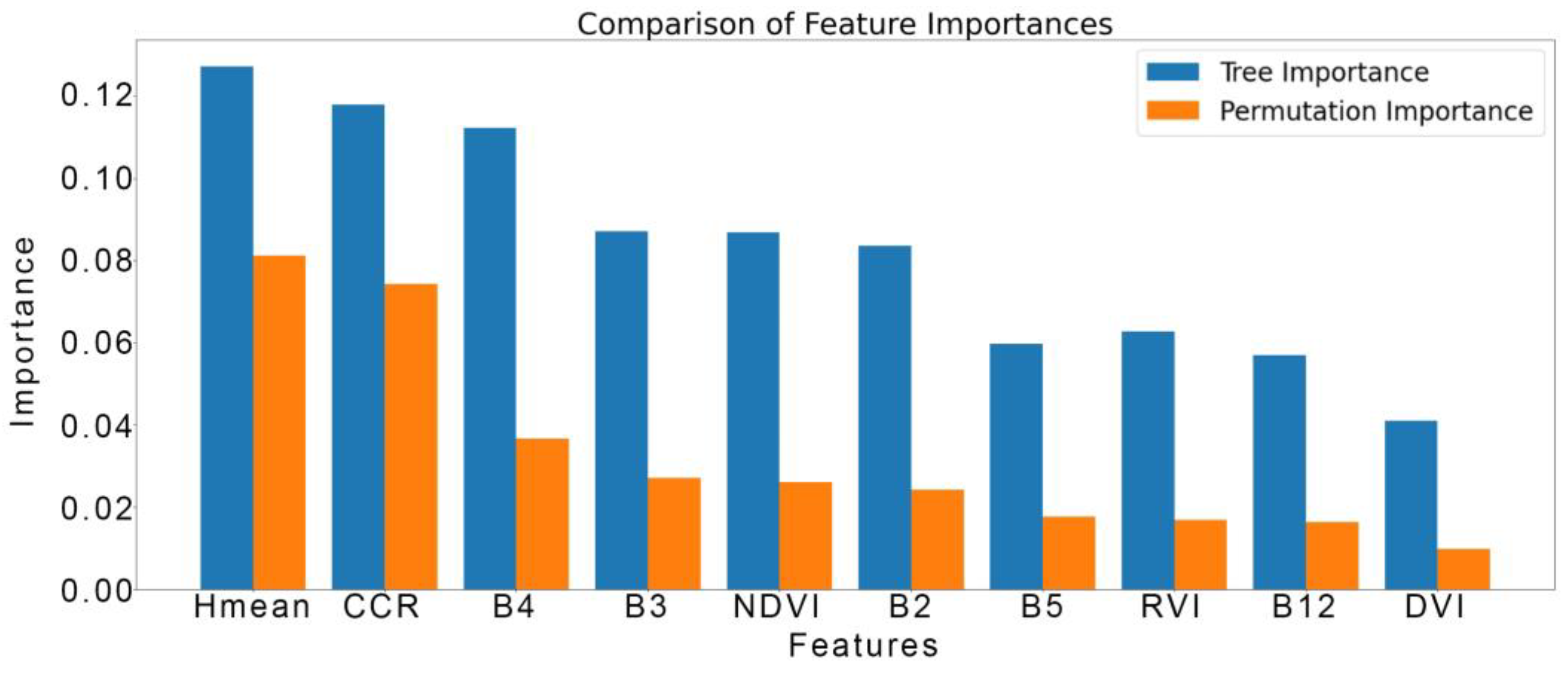
Figure 3 compares feature importance based on tree-based metrics (blue) and permutation scores (orange), using the Boruta algorithm. The evaluated features include structural variables ( H m e a n and CCR), Sentinel-2 bands (B2, B3, B4, B5, B12), and vegetation indices (NDVI, RVI, DVI). Structural features ranked highest, with H m e a n and CCR showing the greatest importance (0.13/0.08 and 0.12/0.07), highlighting their strong explanatory power for AGC. Taller vegetation and denser canopies are typically associated with higher aboveground biomass.
Spectral features ranked lower. For instance, B4 showed a pronounced difference between tree-based and permutation importance, suggesting high collinearity with other bands. While tree-based models can exploit such redundancy, individual predictive contributions decline under permutation. Similar patterns were observed for B3 and NDVI. In contrast, the small difference between the two importance measures for H m e a n and CCR indicates that these 3D features provide unique, non-redundant information critical to AGC estimation.
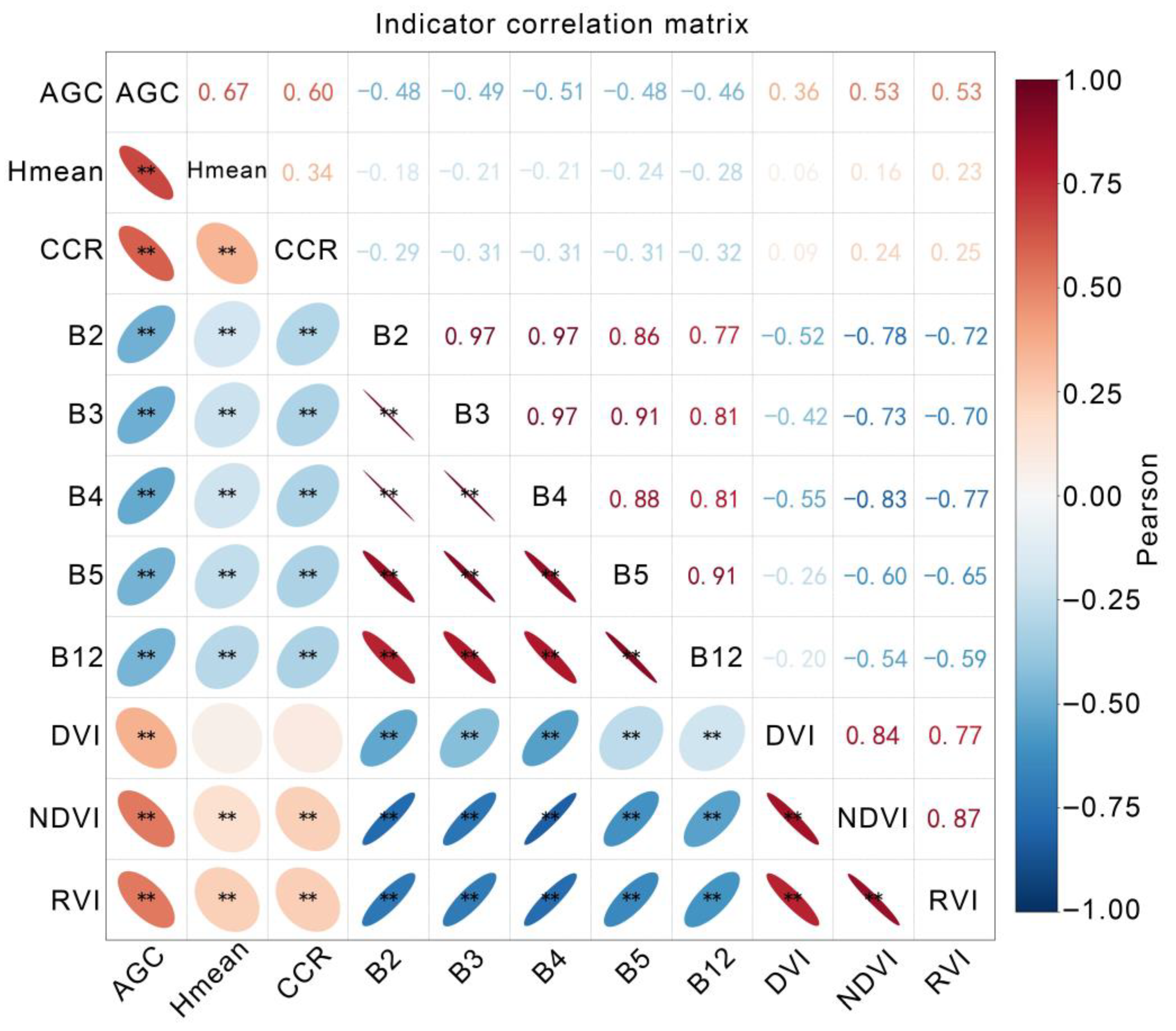
Figure 4 presents the Pearson correlation matrix for key variables, including H m e a n , CCR, Sentinel-2 bands (B2, B3, B4, B5, B12), and vegetation indices (NDVI, RVI, DVI). The ellipsoid plots visualize correlation strength and direction: elongated ellipses denote strong correlations, and color gradients represent the coefficient values (red: positive, blue: negative).
Four main patterns are observed:
(1) H m e a n , CCR, and all vegetation indices show positive correlations with AGC, with H m e a n exhibiting the strongest association. In contrast, bands B2–B5 and B12 are negatively correlated with AGC, underscoring their limited capacity to directly represent aboveground biomass;
(2) Strong inter-correlation among B2–B5 and B12 (e.g., B3–B4 > 0.90), indicating spectral redundancy;
(3) High correlation among NDVI, RVI, and DVI, due to their reliance on red and NIR bands;
(4) Weak-to-moderate correlation between H m e a n /CCR and spectral features, suggesting that structural metrics offer complementary, non-redundant information.

3.2. Model Accuracy Comparison

3.2.1. All-Variable Model

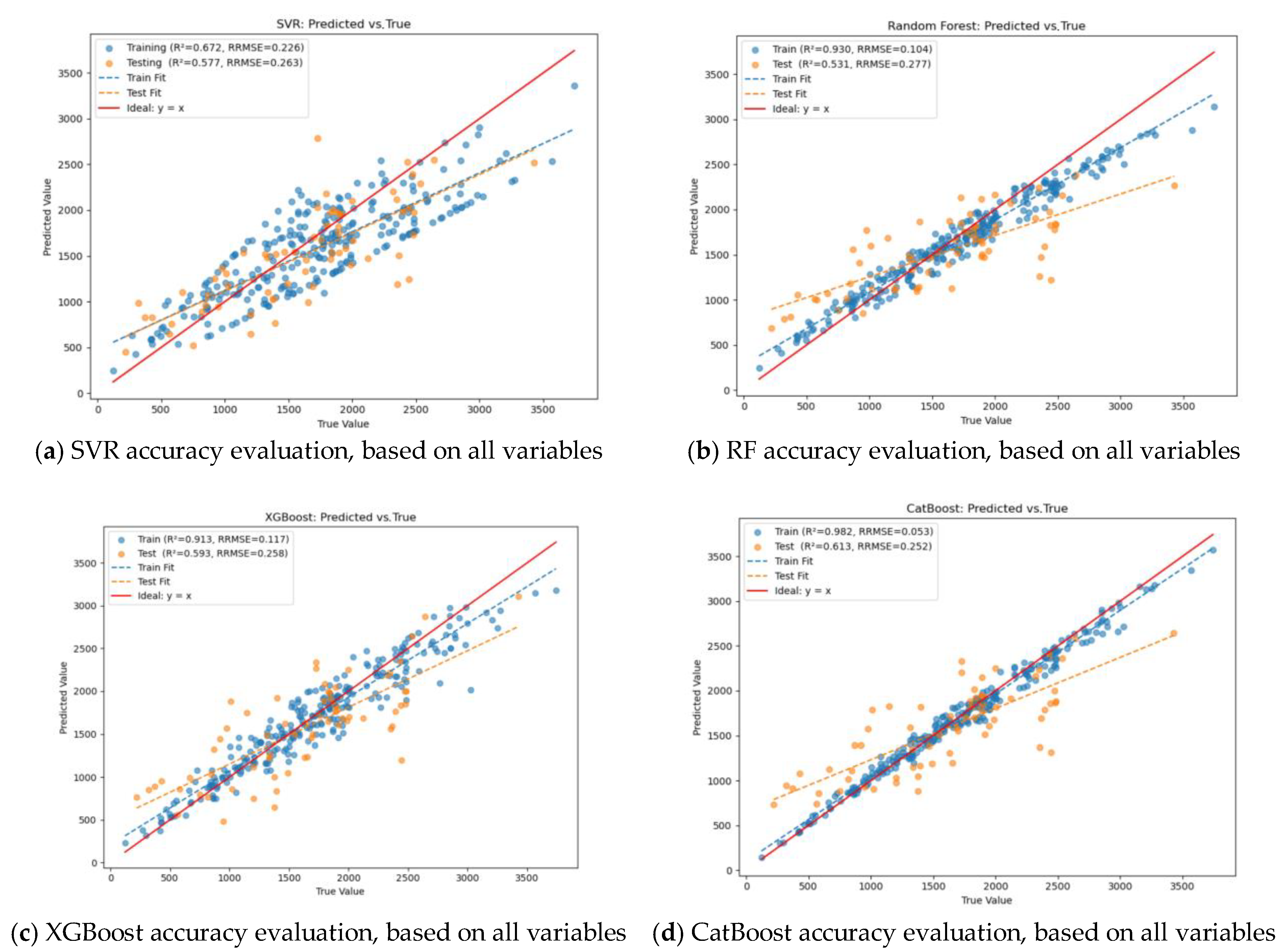
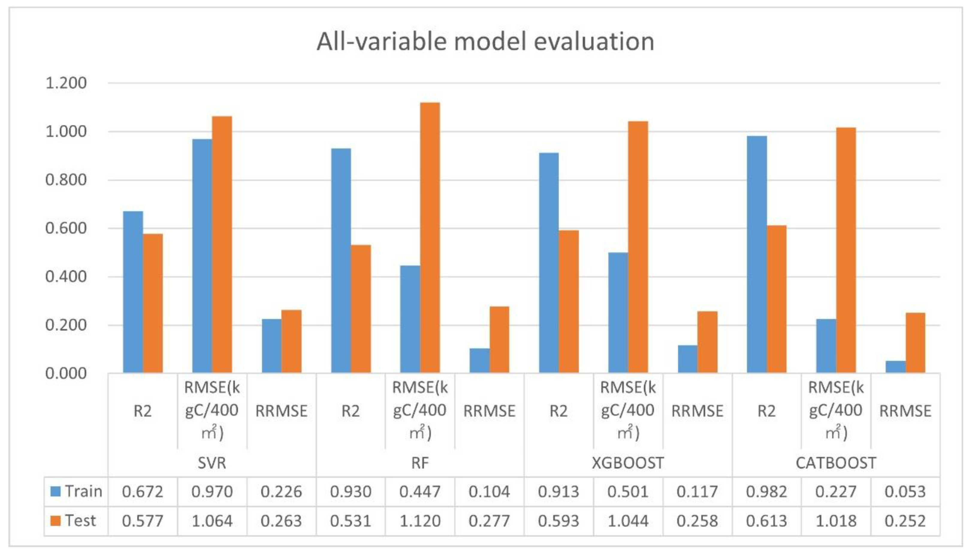
As shown in Figure 5, model performance on the training set followed the order CatBoost > RF > XGBoost > SVR (the scatter plot is shown in Figure A1). Tree-based models (CatBoost, RF, XGBoost) significantly outperformed SVR, confirming their advantage in modeling nonlinear relationships in high-dimensional feature spaces. On the test set, CatBoost achieved the highest R2 and lowest RMSE, followed by XGBoost, while RF and SVR underperformed. All models exhibited some overfitting, with RF showing the largest performance drop (ΔR2 = 0.399) and CatBoost the smallest (ΔR2 = 0.369), indicating CatBoost’s superior generalization in the all-variable scenario.

3.2.2. Spectral Variable Model

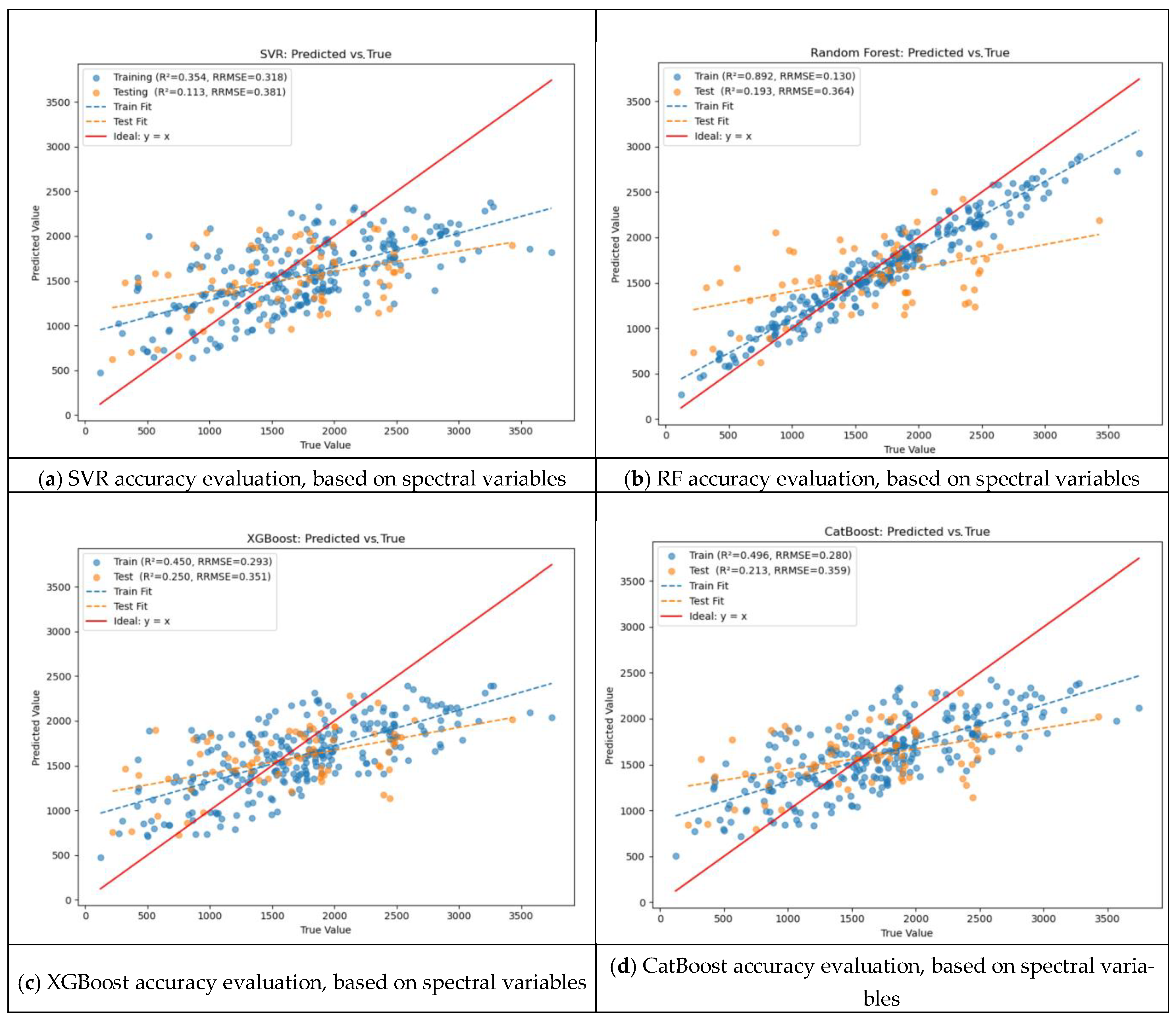
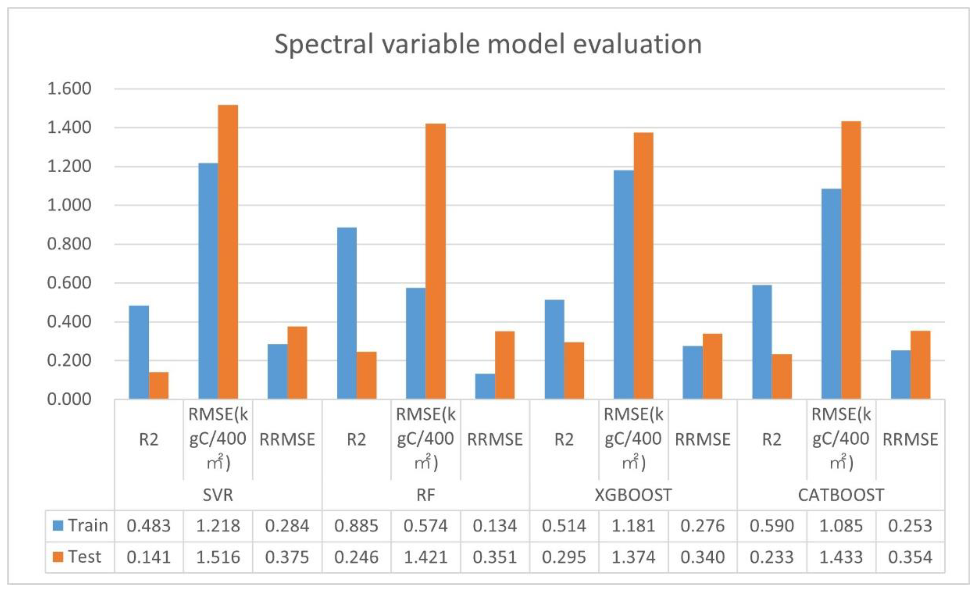
As shown in Figure 6, all models exhibited substantial performance decline when using only spectral indices (the scatter plot is shown in Figure A2). On the training set, RF outperformed others, while the remaining models had R2 values below 0.6, with SVR performing worst. On the test set, R2 dropped to 0.14–0.30, RMSE increased to 1.4–1.5 tC/400 m2, and RRMSE rose to ~35%, indicating that spectral features alone inadequately capture the spatial heterogeneity of AGC. Notably, RF maintained a clear advantage (training R2 nearly 0.31 higher than the next-best model), while XGBoost and CatBoost showed limited gains, likely due to insufficient feature dimensionality. SVR suffered the most severe degradation, highlighting its reliance on high-dimensional, redundant input.

3.2.3. Spectral + Texture Variable Model

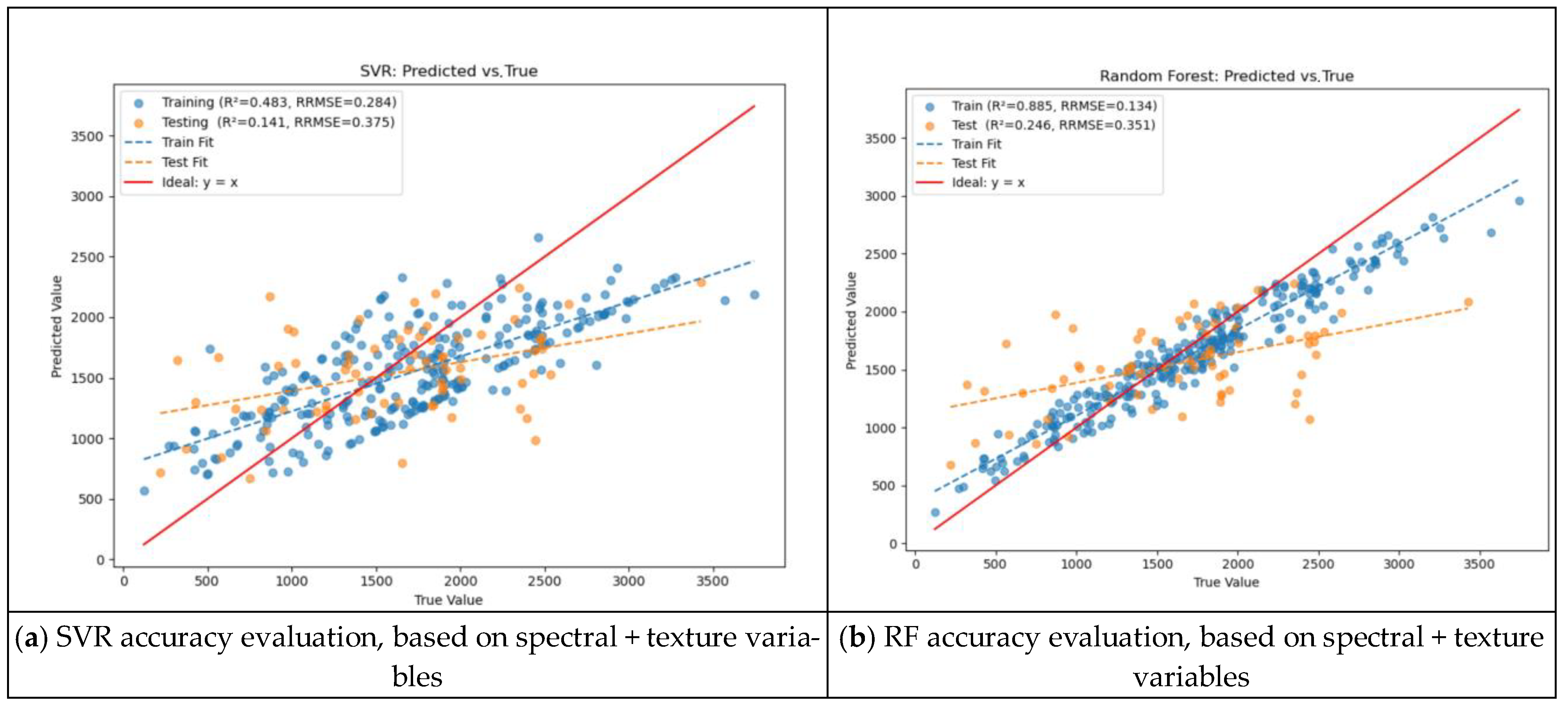
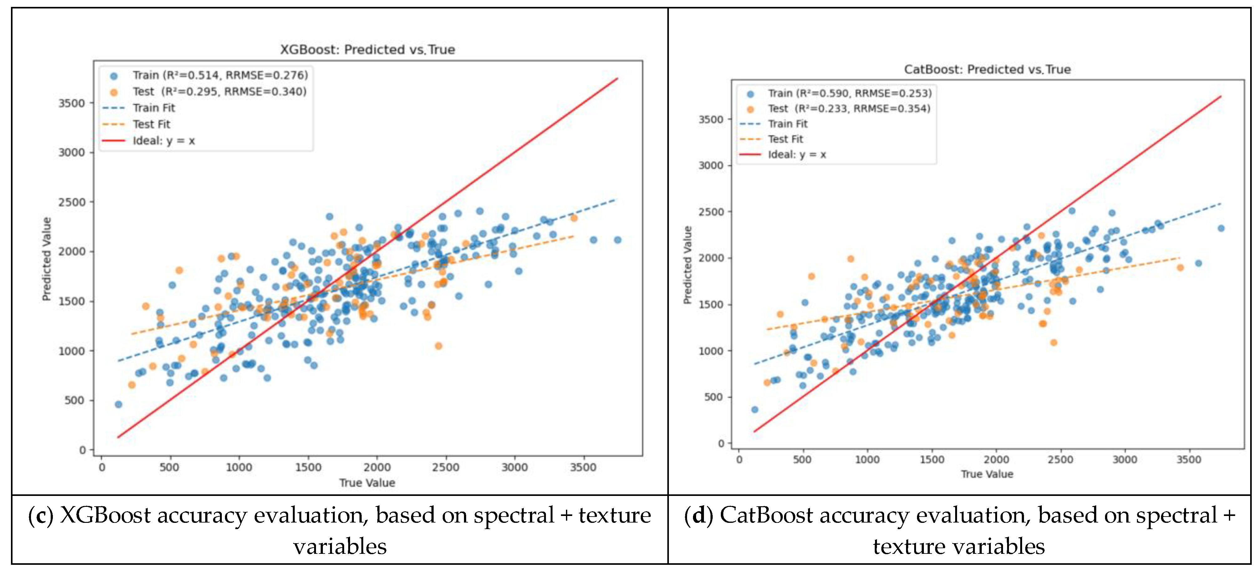
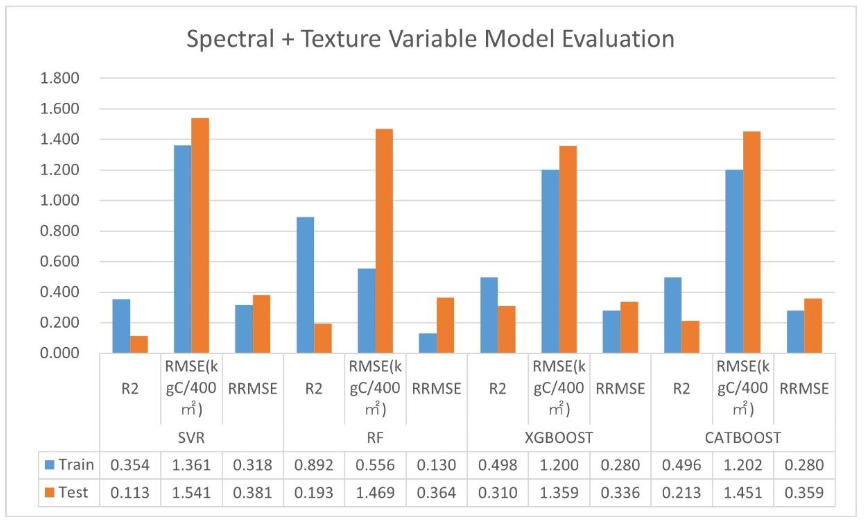
As seen in Figure 7, after adding texture feature variables, the R 2 of RF on the training set slightly improves to 0.892, but CatBoost, XGBoost, and SVR have no significant improvement, which is close to the spectral univariate model. (The scatter plot is shown in Figure A3.). On the test set, the performance of the models does not change much, with the R 2 of XGBoost slightly increasing to 0.310, CatBoost to 0.213, and RF and SVR both slightly lower than 0.20. Vertical comparison reveals that the introduction of texture features does not significantly improve the test results, and it even slightly worsens on some algorithms, suggesting that the selected texture metrics or their complementarities with the spectral model are insufficient, or the existing sample size cannot support the learning of higher-feature dimensions.

3.2.4. Boruta Screened-Variable Model

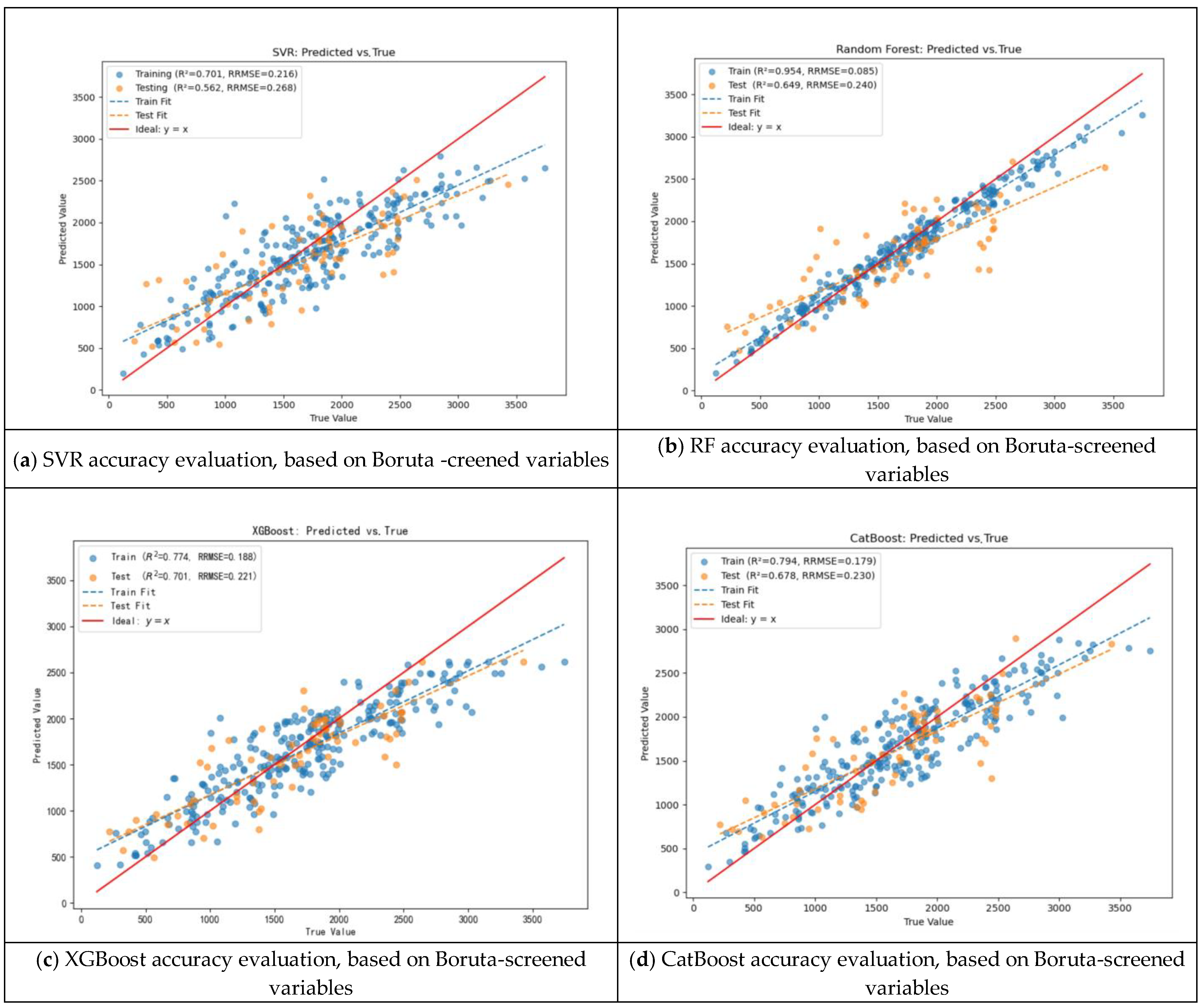
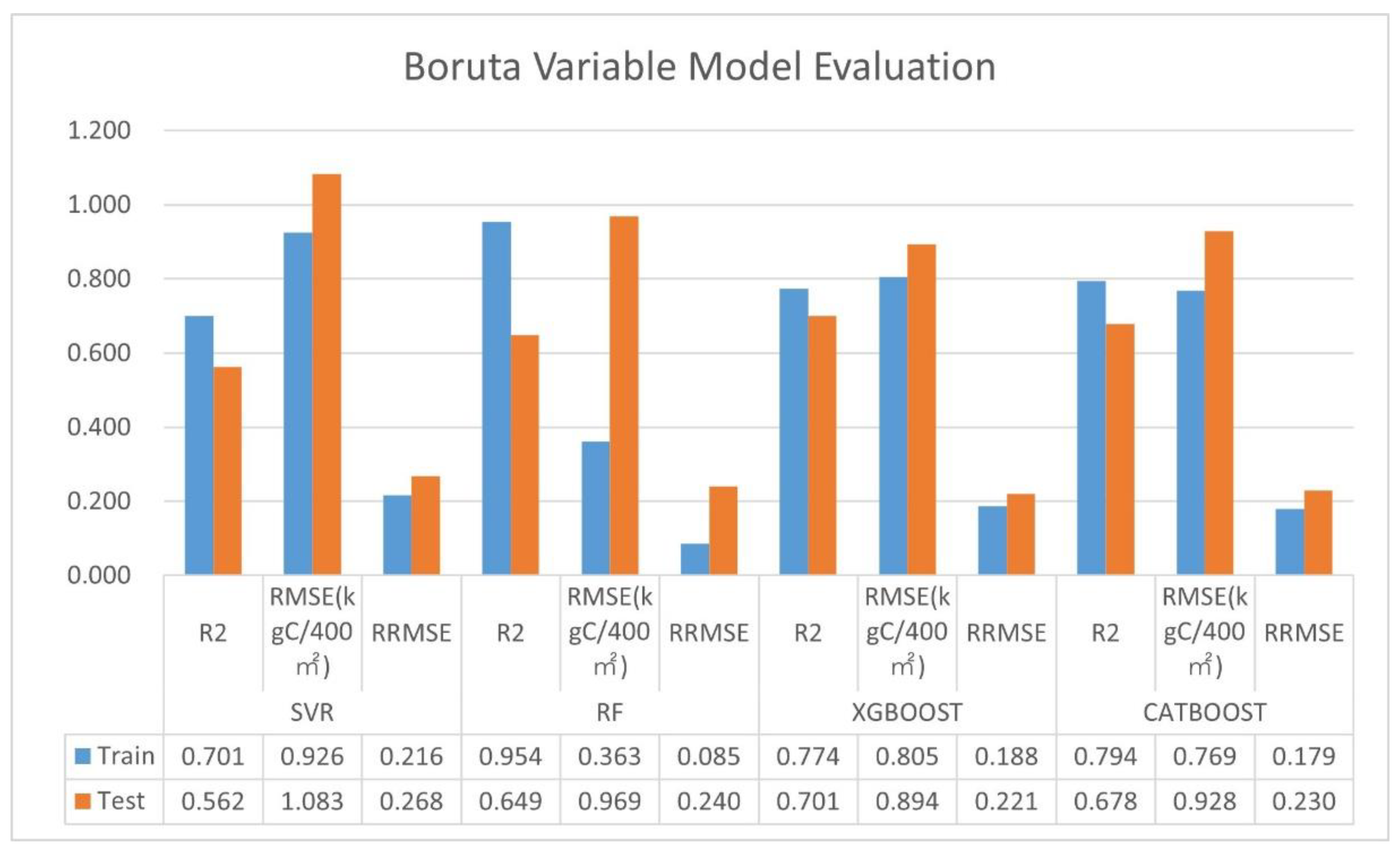
As seen in Figure 8, the subset of key features filtered by Boruta effectively improves the generalization ability of each algorithm. (The scatter plot is shown in Figure A4.) On the training set, the R 2 of RF, XGBoost, and CatBoost are all above 0.77, and, especially, XGBoost reaches 0.774. On the testing set, the R 2 of XGBoost jumps to 0.701, with RMSE = 0.894, and the R 2 of RF and CatBoost are 0.649 and 0.678, respectively, with the testing errors all below 1.1 kgC/ 400 m2. Compared to the fully variable model, the Boruta subset not only reduces overfitting in the training set, but also improves the overall performance of the test set by about 0.09–0.11, demonstrating the value of feature screening in improving model robustness and generalization ability.

3.2.5. The Optimal Model

After the above comparison, it is found that both XGBoost and CatBoost have outstanding performance in different scenarios. Especially after Boruta screening, the R 2 of XGBoost test set is as high as 0.701, which is the best overall performance. Boruta screening significantly improves the model generalization ability, indicating that reasonable feature refinement can reduce overfitting and improve prediction accuracy. Both the all-variable model and the spectral + texture model suffer from different degrees of overfitting, while the single spectrum or the combination of spectrum + texture can hardly meet the demand of high accuracy, and the 3D features and spectra complement each other, to enhance the model performance. Although there is still room for improvement in the R 2 of the best XGBoost model on the test set, this is already a more robust result, with small-sample data [68]. In contrast, the SVR and RF models are less effective in measuring carbon storage, probably due to the small sample size of the dataset and the sensitivity of the two algorithms to noise [69]. Therefore, based on the results of this study, it is recommended to use Boruta screening features to remove redundancy, and the XGBoost algorithm for prediction, to obtain a more robust and accurate carbon storage model for urban vegetation.

3.3. Assessment of the Contribution of Variables

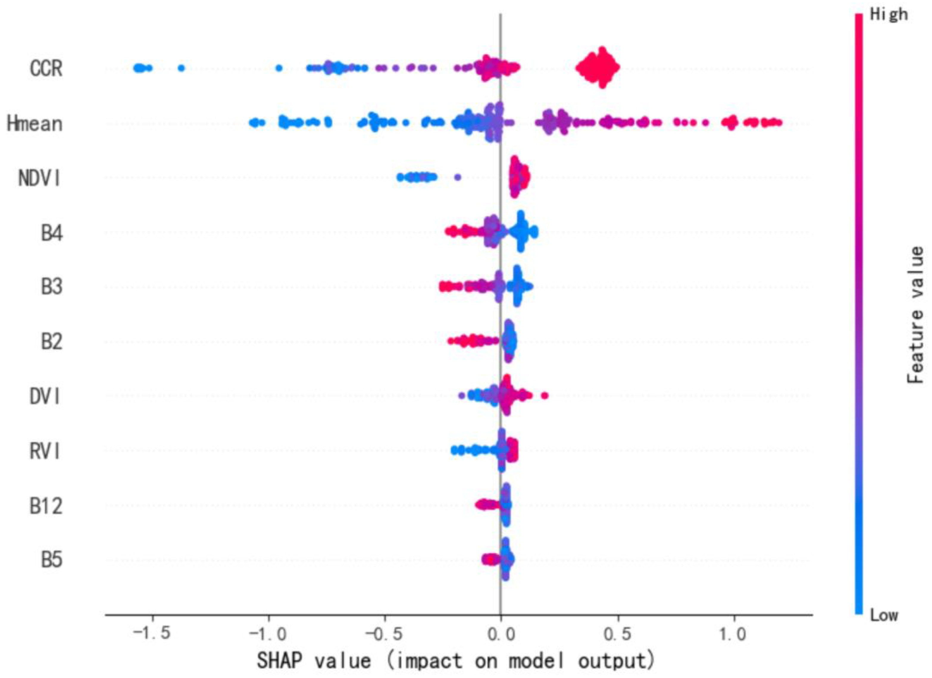
Figure 9 shows the overall contribution of each feature in the model output. As a whole, H m e a n and CCR had the widest range of SHAP values from most negative to most positive. As indicators of 3D structure, they have the most dispersed and laterally extended value points, indicating that this structure has the greatest magnitude of influence on the predicted results. And NDVI ranked third, indicating that the vegetation indices derived from the red edge are still the key spectral signals. The primitive bands (B4, B3, B2) and other indices (DVI, RVI), and SWIR bands (B12, B5) have decreasing contributions. In terms of the contribution of individual variables, a high CCR corresponds to a positive SHAP, which substantially raises the estimate, but the SAHP value is capped at around 0.5, with a threshold effect. Low CCR pulls down the prediction in a negative direction. Similarly, higher tree heights favor positive SHAP values. High NDVI points are distributed in the positive range, indicating that better vegetation growth contributes to greater carbon storage predictions. On the contrary, in the primitive bands such as B4, B3 and B2, the high reflection values are mostly concentrated in the negative SHAP region. This reflects the fact that high band reflections imply low chlorophyll concentration and low carbon storage, whereas low reflections contribute to enhanced prediction.
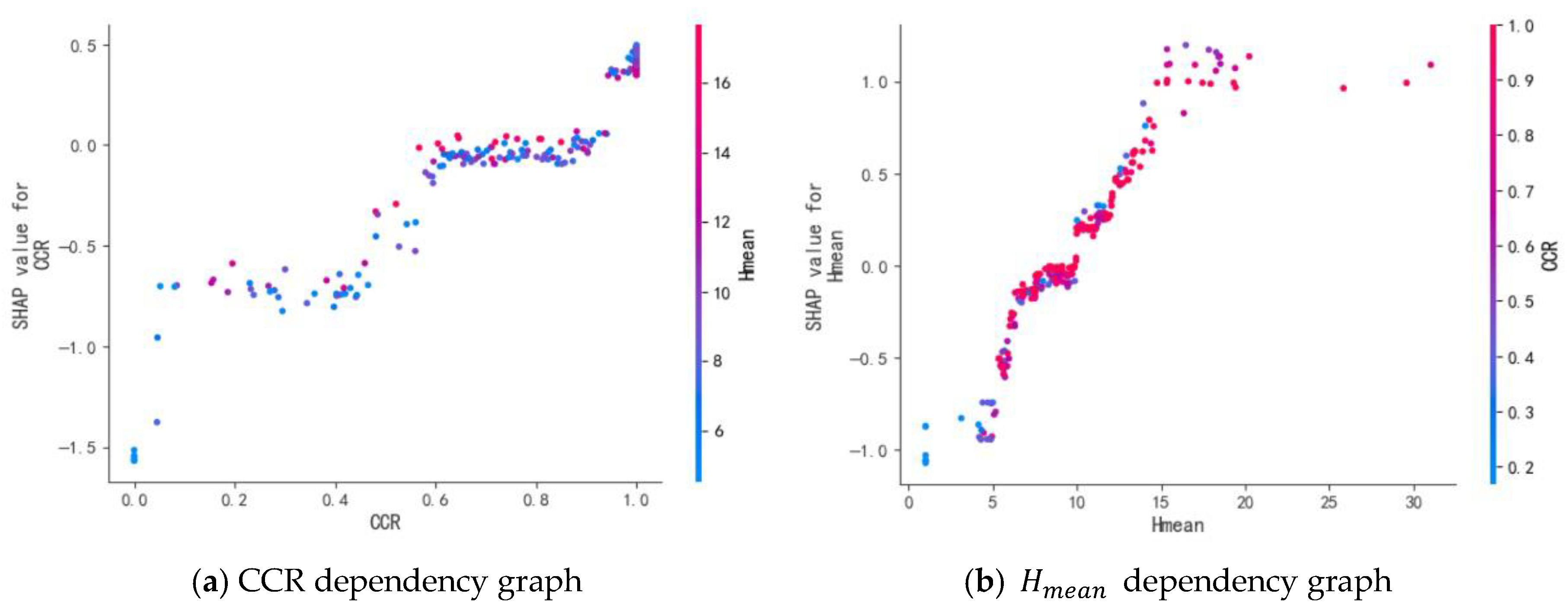
As seen in Figure 10a, the SHAP values generally show a significant upward trend from negative to positive as the CCR rises. At 0.6 ≤ CCR ≤ 0.9, the SHAP value fluctuates around 0, and above 0.9, the SHAP value jumps to 0.5. This phenomenon indicates that lower CCRs have relatively limited, or even slightly negative, contributions to model predictions. However, when the CCR exceeds 0.6, the contribution to carbon storage prediction increases significantly, and, especially when the CCR is 1, it makes a significant contribution to the positive prediction of the model.
As seen in Figure 10b, the SHAP value of H m e a n continued to increase with the growth of H m e a n , with an almost monotonically increasing trend. Especially when H m e a n exceeded 10 m, the increasing trend of SHAP value was more obvious, indicating that the contribution of higher tree communities to carbon storage was more obvious in urban green spaces. However, when H m e a n exceeded about 15 m, SHAP growth leveled off, showing a saturation effect. Thus, the marginal contribution of continued canopy height to carbon storage declined.
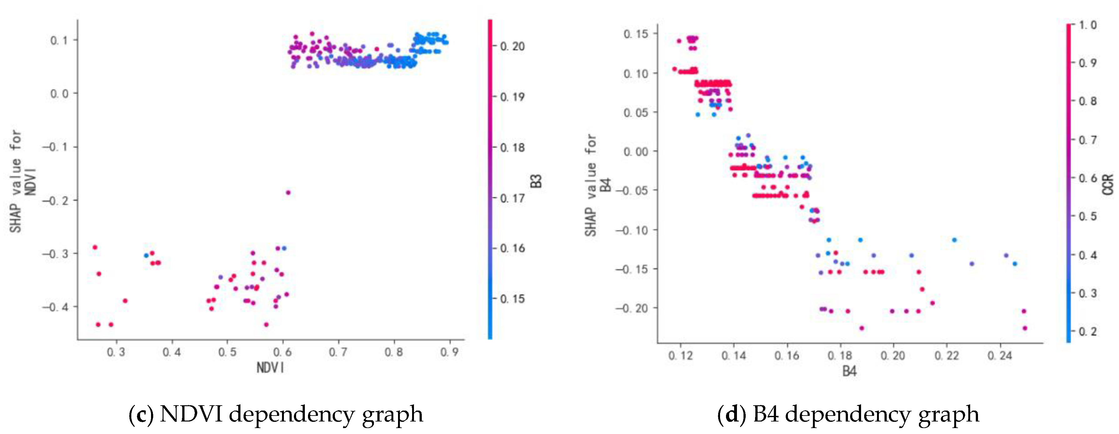
As seen in Figure 10c, SHAP values are negative at NDVI < 0.6, but SHAP jumps directly and continues to stabilize around 0.1 when NDVI exceeds 0.6. This phenomenon suggests that when NDVI exceeds ~0.6, the model begins to interpret the spectral signal as a threshold for appreciable biomass, lifting the carbon storage prediction by positive increments, but the slope slows down significantly to a saturating pattern. With respect to the interaction between NDVI and B3, SHAP is generally positive in the region of high NDVI values. Specifically, when 0.6 < NDVI < 0.8, the interaction with high B3 values is better. However, when NDVI > 0.8, the interaction with low B3 values is better.
As seen in Figure 10d, the SHAP values of B4 generally showed a stepwise decreasing trend, with three distinct phases. When 0.12 < B4 < 0.14, the SHAP value was the highest. When 0.14 < B4 < 0.15, the SHAP value was between −0.10 and 0. When B4 > 0.15, SHAP was all below −0.10. In addition, there was a significant interaction between B4 and CCR, with the highest SHAP values when B4 < 0.14 and CCR > 0.7.

3.4. Model Applications

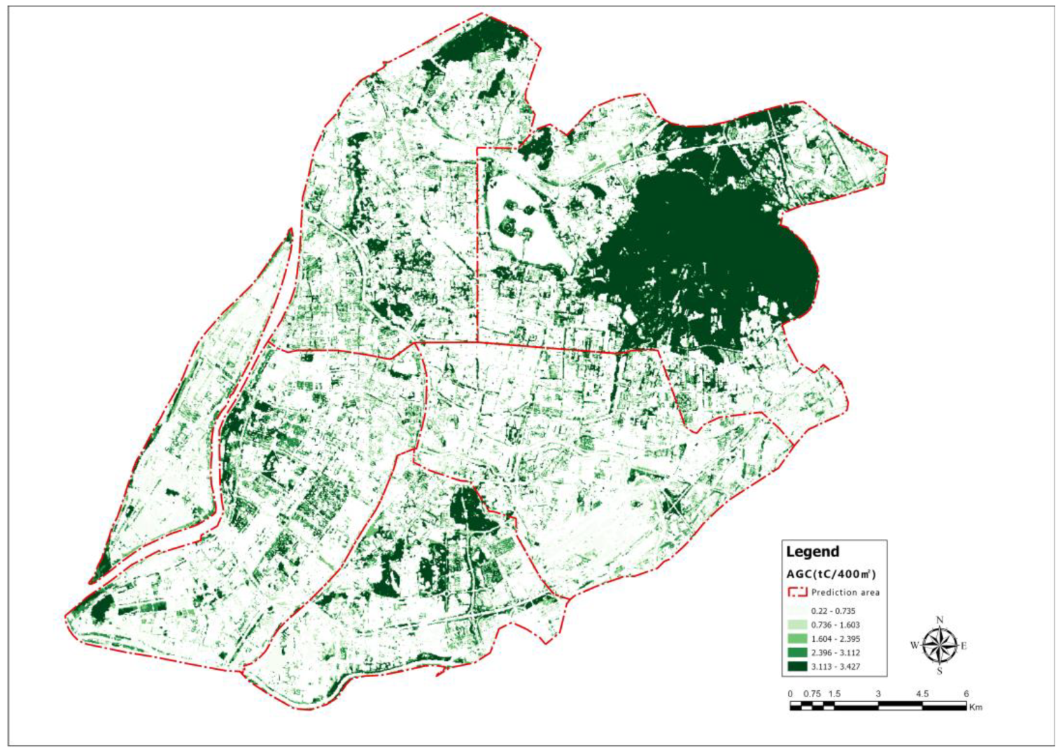
The XGBoost model incorporating Boruta-selected features and 3D structural variables demonstrated the highest predictive accuracy, and was applied to estimate vegetation carbon storage across Nanjing’s central urban area (Figure 11). To assess generalizability, model performance was further evaluated using an independent validation set comprising 40 plots. The results (R2 = 0.811, RMSE = 1.530 tC/400 m2, Bias = −1.104 tC) suggest moderate transferability. The relatively higher validation R2 compared to the test set (R2 = 0.701; RMSE = 0.894) may stem from similarities in vegetation structure, land use, and observation conditions between the training and validation samples. Compared with other urban studies, the study indicating moderate-to-high accuracy. For instance, in Jodhpur, India, XGBoost with Landsat 8 yielded R2 = 0.89, RMSE = 14.08 t/ha [70]; in Buffelsdraai, South Africa, RFR and SVR models with Landsat 8 gave R2 = 0.61, RMSE = 3.56 and R2 = 0.38, RMSE = 6.60, respectively [10]; in Shanghai, China, a Sentinel-2 and Landsat 8 fusion approach achieved R2 = 0.70, RMSE = 6.29 Mg/ha [13]. Although the model exhibits good performance on independent data, further testing is needed for its wider applicability in more diverse urban environments. On the one hand, it reflects the fact that there may be a high degree of similarity between the urban structure and vegetation structure in eastern China. On the other hand, the low-density characteristics of Jodhpur may enhance the accuracy of estimation. It reflects its high spatial heterogeneity, diverse vegetation types, complex land cover, and urban structure, making high-resolution AGC estimation more challenging.
AGC mapping revealed a “high aggregation, low dispersion” spatial pattern. High-density zones are concentrated in mountainous and parkland areas, medium-density zones in established urban neighborhoods, and low-density zones in newly developed regions, particularly Jiangxin Island. This distribution reflects the coupling of Nanjing’s ecological structure—comprising mountains, water bodies, and forest cores—with historical green space development. Areas such as Zijinshan, Mufushan, Xuanwu Lake, and Qingliang Mountain host mature, dense tree cover with high per-unit carbon stocks, whereas low-density zones are often dominated by open grasslands or sparsely vegetated shrublands with limited biomass.

4. Discussion

4.1. Interpretability of the Model

The SHAP analysis revealed a clear pattern in which 3D features—particularly H m e a n and CCR—dominated model predictions, while spectral features played a secondary, complementary role. This result aligns well with both the Pearson correlation analysis and feature importance rankings, reinforcing the model’s stability and interpretability. Notably, the correlation between H m e a n /CCR and all spectral indices was below 0.35, indicating statistical orthogonality. While spectral reflectance primarily captures leaf-level properties such as chlorophyll or water content, 3D metrics reflect canopy structure and biomass, making them critical for AGC estimation. Their complementarity enhances model performance, enabling accurate carbon mapping even under complex urban conditions.
The SHAP dependence plots further clarify individual feature effects. The shape correlation diagram further illustrates the influence of each feature. When CCR > 0.5, it shows a positive contribution, and when CCR = 1, the positive contribution is the largest, but it stops at 0.5. This reflects the common saturation effect in dense urban vegetation. High canopy coverage usually corresponds to higher aboveground biomass (AGC). However, high CCR means that understory biomass may not be recognized, so it has a positive contribution to the model. [34]. In contrast, H m e a n showed a wider and more linear SHAP value distribution. Greater tree height was consistently associated with higher AGC predictions, reinforcing its biological link to biomass accumulation. Interaction effects between CCR and H m e a n revealed a synergistic influence: plots with both high canopy cover and tall trees exhibited significantly higher predicted carbon storage, consistent with patterns reported in previous studies [71]. From a model mechanics perspective, tree-based algorithms such as XGBoost prioritize high-gain splits, and samples with large CCR or H m e a n are often selected in early tree nodes, amplifying their predictive weight [72].
The performance gap between 3D and texture features was also evident. While previous studies [13,70] reported high R2 using spectral–texture combinations in relatively homogenous green areas such as forests or agricultural fields, this study found that texture metrics alone failed to provide robust predictions in highly fragmented urban landscapes. This discrepancy likely stems from Sentinel-2′s limited spatial resolution, which restricts the utility of texture descriptors in complex urban mosaics.
In summary, 3D features serve as primary drivers of AGC estimation in urban environments, with spectral features providing additional but non-redundant support. Their joint use enables more accurate modeling of vegetation carbon storage under structurally diverse urban conditions.

4.2. Estimated Effects of Different Green Spaces

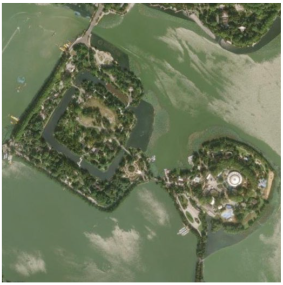
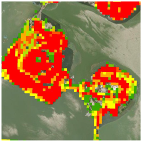
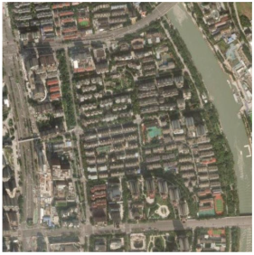
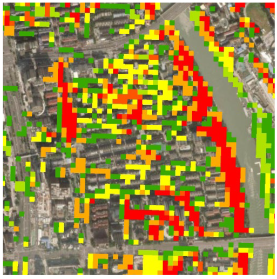
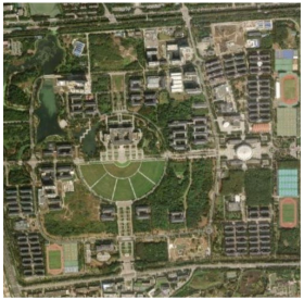
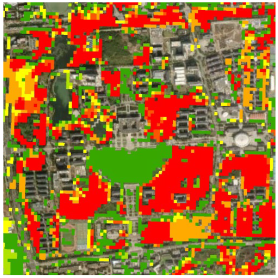
To assess model performance within different urban contexts, predicted carbon storage was visually compared with high-resolution satellite imagery (Table 1). In park green spaces, the model effectively distinguished between high, medium, and low AGC zones, demonstrating strong discrimination between tree-dominated and grass-dominated communities. However, small-scale open-water bodies were occasionally misclassified as high-carbon areas. This overestimation likely stems from their low reflectance in red and NIR bands [73], which—when combined with a flat surface—may mimic the spectral–structural profile of “high CCR + low B4,” leading to false-positive AGC contributions in SHAP interpretations.
At Sentinel-2′s 10 m resolution, mixed pixels are common, especially in fragmented green spaces [74]. Spectral and structural mixtures—such as “vegetation + pavement,” “shrubs + soil,” or “trees + water”—introduce uncertainty by blending reflectance and canopy height values, thereby biasing model outputs [75]. These effects are particularly pronounced in narrow or heterogeneous urban environments [76].
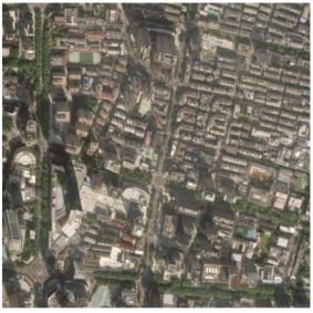
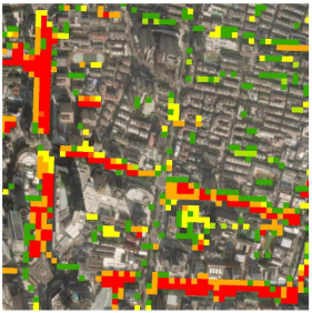
In roadside, residential, and campus green spaces, the model delineated vegetation boundaries relatively well, even in proximity to hard surfaces. However, inconsistencies were observed in predicted AGC among street trees of similar species and size. This variability can be attributed to shadow effects caused by nearby buildings, which reduce visible reflectance and NDVI, and may lower canopy height measurements from satellite LiDAR, due to diminished signal return [77,78]. Consequently, shaded trees tend to receive lower AGC estimates than those in sunlit areas, despite comparable biomass.
Overall, the model performs best in large, continuous green spaces such as parks, where vegetation stands are well-defined and less affected by mixed land cover or urban interference. Its accuracy will decline in the environment of spatial dispersion or on a small scale. These findings highlight the importance of considering context-specific urban morphology when applying AGC models.

4.3. Research Limitations and Perspectives

This study improves previous modeling efforts by integrating multi-source 3D vegetation features to enhance the representation of urban structure in carbon storage estimation [79]. However, urban-vegetation carbon dynamics are influenced by a wider range of factors—such as soil conditions, species diversity, and management intensity—that were not fully captured in this model. While the selected structural and spectral variables cover key dimensions, essential ecological attributes like vegetation stratification remain unobservable, due to current satellite 3D data limitations [80].
Although H m e a n derived from GEDI data may contain a small bias due to temporal mismatch with Sentinel-2 imagery, the expected growth of mature urban trees (0.15–0.35 m/year) over four years corresponds to only 0.60–1.40 m [81,82,83]. Given GEDI’s vertical resolution (~1 m) [84], this difference is within the measurement uncertainty. Consequently, the bias in H m e a n is unlikely to cause substantial deviation in biomass estimates, especially when combined with other structural and spectral predictors in the model.
The structural complexity commonly found in urban areas—such as shadows, obstructions, and vegetation heterogeneity—is not explicitly accounted for in the model, which may affect its accuracy [85]. Although the stratified sampling strategy ensures species-level representativeness, the model’s robustness can be improved by expanding the sample size and incorporating more complex environments (such as shaded areas or mixed-use areas). The model was trained exclusively on the central area of Nanjing, limiting its direct transferability to cities with different ecological and urban morphologies. Future studies could further address this issue by integrating shadow detection and correction techniques, to reduce underestimation in shaded vegetation areas and improve the robustness of urban AGC estimation. And, also, we will utilize SHAP interaction plots to better understand feature dependencies and enhance the model’s robustness in real-world environments [86]. Additionally, although the model relies on widely used features (e.g., canopy height, coverage, and vegetation indices), its performance may vary due to differences in species composition, climate, and landscape configuration caused by regional differences [36]. Therefore, future research will focus on cross-city validation, to assess the model’s generalization ability.

5. Conclusions

This study developed a high-accuracy urban-vegetation carbon storage model by integrating 3D structural and spectral features using the Boruta algorithm and XGBoost. Results highlight the dominant role of 3D features in reducing estimation bias and improving model performance. The research advances carbon modeling by addressing structural complexity through remote sensing fusion, and contributes a scalable tool for urban carbon assessment. The model offers practical support for green space planning and provides a methodological reference for data-driven urban carbon accounting.

Author Contributions

Conceptualization, Y.F. and Y.C. (Yuning Cheng); methodology, Y.F.; software, Y.F. and Y.C. (Yilun Cao); validation, Y.F. and Y.C. (Yilun Cao); formal analysis, Y.F.; investigation, Y.F. and Y.C. (Yilun Cao); resources, Y.F.; data curation, Y.F. and Y.C. (Yilun Cao); writing—original draft preparation, Y.F.; writing—review and editing, Y.C. (Yuning Cheng); visualization, Y.F.; supervision, Y.C. (Yuning Cheng); project administration, Y.C. (Yuning Cheng); funding acquisition, Y.C. (Yuning Cheng). All authors have read and agreed to the published version of the manuscript.

Funding

This research was funded by the Key Program of the National Natural Science Foundation of China, grant number 51838003, which provided sufficient financial support.

Data Availability Statement

Data will be made available upon request.

Conflicts of Interest

The authors declare no conflicts of interest.

Appendix A

Table A1. Sample site selection and number of communities.
Type of Green SpaceName of Green SpaceNo.Number of Communities
Park green spaceComprehensive Park
(waterfront)
Xuanwu Lake Park160
Mochou Lake Park230
Crescent Lake Park320
Xiuqiu Park420
Little Peach Park520
Comprehensive Park
(Mountain)
Qingliang mountain—Stone city Park630
Arctic Pavilion Park720
Neighborhood parkPeace Park810
Specialty parkHexi Qingao Forest Park (other specialized parks)930
Nanjing China Greening Expo Park (other specialized parks)1035
Hexi Ecological Park (other specialized parks)1130
Xi’anmen Ruins Park (Specialized ruins park)1215
Plaza green space Daxinggong Civic Plaza135
Drum Tower Plaza1410
Affiliated green spaceCampusSipalou Campus of Southeast University1515
CommercialJinling Riverside Hotel1615
ResidentialCui Ping Dong Nan1720
Regional green spaceScenicYuhuatai Scenic Area1820
WetlandsFish Mouth Wetland Park1930
Table A2. Plot community types and numbers.
No.Community TypeCanopy LevelQuantities
1pure forest community evergreen broadleafSingle layer16
2evergreen conifersSingle layer5
3deciduous broadleafSingle layer20
4deciduous conifersSingle layer5
5mixed forest communitymixed evergreen and deciduous broadleavesSingle layer11
6Multilayer200
7mixed evergreen and deciduous conifersSingle level2
8evergreen and deciduous mixed conifers and broadleavesMultilayer81
9deciduous mixed coniferMultilayer19
10evergreen mixed coniferMultilayer6
11No tree communitiesLawns, Ground Covers and ShrubsCrownless10
Total375
Table A3. The growth equations of common trees in Nanjing area with different speeds. (footer: / represents no equation available).
Species Trunk   Biomass   ( B t ) (kg)Branch Biomass ( B b r ) (kg)Leaf Biomass
( B l ) (kg)
Bark Biomass
( B b a ) (kg)
Aboveground Biomass (AGB) (kg)Modeling Area
Cupressus funebris//// A G B = 0.02479 D 2.0333 Jiangsu [87]
Pinus thunbergii//// A G B = 0.0462
( D 2 H ) 0.9446
Anhui [87]
Pinus massoniana//// B g 2 = 0.06 H 0.7934 D 1.8005  
B g 3 = 0.137708 H 1.487266
L 0.405207  
A G B = B g 2 + B g 3
Zhejiang [88]
Cunninghamia lanceolata//// B g 2 = 0.0647 H 0.8959 D 1.488  
B g 3 = 0.097 D 1.7814 L 0.0346  
A G B = B g 2 + B g 3
Zhejiang [88]
Cryptomeria fortunei B t = 0.2716
D 2 H 0.7379
B b r = 0.0326
( D 2 H ) 0.8472
B l = 0.0250
( D 2 H ) 0.7328
B b a = 0.0379
( D 2 H ) 0.7328
A G B = B t + B b r + B l + B b a Jiangsu [87]
Metasequoia glyptostroboides B t = 0.656 + 0.028 D 2 H B b r = 1.258 + 0.007 D 2 H B l = 0.004 + 0.001 D 2 H B b a = 0.135 + 0.003 D 2 H A G B = B t + B b r + B l + B b a Jiangsu [87]
Cinnamomum camphora//// A G B = 0.00751
( D 2 H ) 1.2675
Shanghai [87]
Robinia pseudoacacia B t = 0.0681
( D 2 H ) 0.9865
B b r = 12.020 + 0.009 D 2 H B l = 0.549 + 0.007 D 2 H B b a = 4.217 + 0.008 + 0.007 D 2 H A G B = B t + B b r + B l + B b a Jiangsu [87]
Elaeocarpus decipiens//// A G B = 0.00015
( D 2 H ) 1.28808
Shanghai [87]
Quercus spp. B t = 0.3108
( D 2 H ) 0.67428
B b r = 0.0293
( D 2 H ) 0.75662
B l = 0.0922
( D 2 H ) 0.39445
B b a = 0.93685
( D 2 H ) 0.614021
A G B = B t + B b r + B l + B b a Henan [87]
Ulmus spp. B t = 0.0709 D 2.42 B b r = 4.924 D 0.976 B l = 0.0922
( D 2 H ) 0.39445
B b a = 1.163 D 0.64 A G B = B t + B b r + B l + B b a Liaoning [87]
Ligustrum lucidum//// A G B = 0.08685
( D 2 H ) 0.89923
Shanghai [87]
Magnolia grandiflora//// A G B = 0.267867
( D 2 H ) 0.71442
Shanghai [87]
Hard broadleaf species//// A G B = 0.03451
( D 2 H ) 1.0037
Zhejiang [88]
Populus spp. B t = 0.0074046
( D 2 H ) 1.069
B b r = 0.0041773 ( D 2 H ) 0.9911 B l = 0.071532
( D 2 H ) 0.4489
/ A G B = B t + B b r + B l Jiangsu [87]
Paulownia spp. B t = 0.01693
( D 2 H ) 0.9234
B b r = 0.00247
( D 2 H ) 1.0977
B l = 0.145
( D 2 H ) 0.7156
B b a = 0.004105
( D 2 H ) 0.9296
A G B = B t + B b r + B l + B b a Anhui [87]
Koelreuteria bipinnata//// B g = 0.02173
( D 2 H ) 1.08777
Shanghai [87]
Liriodendron chinense//// B g = 0.00950
( D 2 H ) 1.7994
Shanghai [87]
Soft broadleaf species/Softwood broadleaves//// B g 2 = 0.044 H 0.7197
D 1.7095  
B g 3 = 0.0856 D 1.22657
L 0.3970  
A G B = B g 2 + B g 3
Zhejiang [88]
Eucommia ulmoides B t = 0.118194 D 2.047788 B b r = 0.013137 D 2.919738 B l = 0.033970 D 0.001548 / A G B = B t + B b r + B l Henan [87]
Ginkgo biloba//// B g = 0.118604
( D 2 H ) 0.8237
Shanghai [87]
Mixed broadleaf species//// B g = 0.17322 D 2.3458 Guizhou [87]
Phyllostachys edulis//// B g = 0.0712
( D 2 H ) 0.7066
Shanghai [87]
Prunus persica (D = ground diameter)//// B g = 0.18241 D 2.0558 Shanghai [87]
Shrub cluster Shrub layer//// Zhejiang [88]
Conifers//// B g = 0.0326335
( D 2 H ) 0.9472
National [87]
Broadleaves//// B g = 0.1191632
( D 2 H ) 0.8542
National [87]
Table A4. Carbon content factors (CFs) of common vegetation in Nanjing.
Tree SpeciesCFTree SpeciesCF
Pinus sylvestris var. mongolica0.486 [89]Betula platyphylla0.506 [89]
Pinus yunnanensis0.508 [89]Eucalyptus spp.0.525 [89]
Pinus kesiya var. langbianensis0.501 [89]Firmiana simplex0.423 [89]
Pinus elliottii0.474 [89]Platanus × acerifolia0.441 [89]
Pinus massoniana0.525 [89]Acer spp.0.45 [89]
Larix gmelinii0.489 [89]Ginkgo biloba0.447 [89]
Pinus hwangshanensis0.506 [89]Sapindus mukorossi0.435 [89]
Pinus taeda0.511 [89]Koelreuteria paniculata0.424 [89]
Pinus armandii0.523 [89]Celtis sinensis0.422 [89]
Pinus densata0.501 [89]Liquidambar formosana0.418 [89]
Pinus koraiensis0.511 [89]Bischofia polycarpa0.436 [89]
Pinus thunbergii0.515 [89]Schima superba0.471 [89]
Pinus tabuliformis0.517 [89]Michelia chapensis0.443 [89]
Pinus densiflora0.515 [89]Alnus trabeculosa0.45 [89]
Cedrus deodara0.454 [89]Populus tomentosa0.471 [89]
Quercus spp.0.48 [89]Populus spp.0.43 [89]
Betula spp.0.487 [89]Salix matsudana0.432 [89]
Picea spp.0.49 [89]Salix spp.0.465 [89]
Abies spp.0.496 [89]Ulmus spp.0.421 [89]
Cryptomeria fortunei0.514 [89]Sophora japonica0.444 [89]
Metasequoia glyptostroboides0.439 [89]Robinia spp.0.502 [89]
Cunninghamia lanceolata0.446 [89]Prunus salicina0.44 [89]
Sabina chinensis0.45 [89]Prunus spp.0.46 [89]
Cunninghamia lanceolata0.499 [89]Prunus armeniaca0.43 [89]
Cupressus spp.0.485 [89]Pyrus spp.0.46 [89]
Tilia spp.0.475 [89]Syringa spp.0.43 [89]
Machilus pingii0.485 [89]Malus spp.0.45 [89]
Cinnamomum spp.0.434 [89]Forsythia spp.0.43 [89]
Magnolia spp.0.434 [89]Broadleaf species0.48 [89]
Osmanthus fragrans0.434 [89]Coniferous species0.489 [89]
Fraxinus chinensis0.488 [89]
Table A5. Feature-variable types and descriptions.
TypeNameCalculation Models or DescriptionsRemarks
Spectral featureCoastalBand1
BlueBand2
GreenBand3
RedBand4
Red-edge1Band5
Red-edge2Band6
Red-edge3Band7
NIR1Band8
NIR2Band8A
Swir1Band9
Swir2Band11
Swir3Band12
DVINIR-R
NDVI N I R R / N I R + R
EVI 2.5 * N I R R / N I R + 6 × R 7.5 × B L U E + 1
RVI N I R / R
Texture featureMean i = 0 N j = 0 N p i , j × i There are five window sizes for texture feature extraction: 3 × 3, 5 × 5, 7 × 7, 9 × 9, 11 × 11
Variance i = 0 N j = 0 N p i , j × i M e a n 2
Homogeneity i = 0 N j = 0 N p i , j × 1 1 + i j 2
Contrast i = 0 N j = 0 N p i , j × i j 2
Dissimilarity i = 0 N j = 0 N p i , j i j
Entropy i = 0 N j = 0 N p i , j log p i , j
Second moment i = 0 N j = 0 N p i , j 2
Correlation i = 0 N j = 0 N M e a n × j M e a n × p i , j V a r i a n c e
3D feature H m e a n H m e a n = i = 0 n H i n Average of tree heights within a 20 m grid
CCR C C R = i = 0 n C C A A Percentage of canopy area within a 20 m grid
Figure A1. Scatter plot of predicted values and actual values for the four models under input, with all variables.
Forests 16 01381 g0a1
Figure A2. Scatter plots of predicted values and actual values for four models under input, with spectral variables.
Forests 16 01381 g0a2
Figure A3. Scatter plot of predicted values and actual values for four models under the input of spectral + texture variables.
Forests 16 01381 g0a3aForests 16 01381 g0a3b
Figure A4. Scatter plots of predicted values and actual values for four models with variables filtered by Boruta.
Forests 16 01381 g0a4

References

  1. Ge, J.; Wang, Y.; Zhou, D.; Gu, Z.; Meng, X. Effects of urban vegetation on microclimate and building energy demand in winter: An evaluation using coupled simulations. Sust. Cities Soc. 2024, 102, 105199. [Google Scholar] [CrossRef]
  2. Zheng, X.; Zhang, N.; Wang, X. Development of a modified thermal humidity index and its application to human thermal comfort of urban vegetation patches. Ecosyst. Health Sustain. 2022, 8, 2130095. [Google Scholar] [CrossRef]
  3. Diener, A.; Mudu, P. How can vegetation protect us from air pollution? A critical review on green spaces’ mitigation abilities for air-borne particles from a public health perspective-with implications for urban planning. Sci. Total Environ. 2021, 796, 148605. [Google Scholar] [CrossRef] [PubMed]
  4. Zhao, D.; Cai, J.; Xu, Y.; Liu, Y.; Yao, M. Carbon sinks in urban public green spaces under carbon neutrality: A bibliometric analysis and systematic literature review. Urban For. Urban Green. 2023, 86, 128037. [Google Scholar] [CrossRef]
  5. Stroud, S.; Peacock, J.; Hassall, C. Vegetation-based ecosystem service delivery in urban landscapes: A systematic review. Basic Appl. Ecol. 2022, 61, 82–101. [Google Scholar] [CrossRef]
  6. Ma, J.; Li, X.; Baoquan, J.; Liu, X.; Li, T.; Zhang, W.; Liu, W. Spatial variation analysis of urban forest vegetation carbon storage and sequestration in built-up areas of Beijing based on i-Tree Eco and Kriging. Urban For. Urban Green. 2021, 66, 127413. [Google Scholar] [CrossRef]
  7. Liu, C.; Liu, Z.; Xie, B.; Liang, Y.; Li, X.; Zhou, K. Decoupling the effect of climate and land-use changes on carbon sequestration of vegetation in Mideast Hunan Province, China. Forests 2021, 12, 1573. [Google Scholar] [CrossRef]
  8. Zhang, Y.; Shao, Z. Assessing of urban vegetation biomass in combination with LiDAR and high-resolution remote sensing images. Int. J. Remote Sens. 2021, 42, 964–985. [Google Scholar] [CrossRef]
  9. Sonti, N.F.; Groffman, P.M.; Nowak, D.J.; Henning, J.G.; Avolio, M.L.; Rosi, E.J. Urban net primary production: Concepts, field methods, and Baltimore, Maryland, USA case study. Ecol. Appl. 2022, 32, e2562. [Google Scholar] [CrossRef]
  10. Yang, K.; Zhou, P.; Wu, J.; Yao, Q.; Yang, Z.; Wang, X.; Wen, Y. Carbon stock inversion study of a carbon peaking pilot urban combining machine learning and Landsat images. Ecol. Indic. 2024, 159, 111657. [Google Scholar] [CrossRef]
  11. Zhao, M.; He, Z.; Du, J.; Chen, L.; Lin, P.; Fang, S. Assessing the effects of ecological engineering on carbon storage by linking the CA-Markov and InVEST models. Ecol. Indic. 2019, 98, 29–38. [Google Scholar] [CrossRef]
  12. Chen, L.; Wang, Y.; Zhu, E.; Wu, H.; Feng, D. Carbon storage estimation and strategy optimization under low carbon objectives for urban attached green spaces. Sci. Total Environ. 2024, 923, 171507. [Google Scholar] [CrossRef] [PubMed]
  13. Li, H.; Zhang, G.; Zhong, Q.; Xing, L.; Du, H. Prediction of urban forest aboveground carbon using machine learning based on landsat 8 and Sentinel-2: A case study of Shanghai, China. Remote Sens. 2023, 15, 284. [Google Scholar] [CrossRef]
  14. Pregitzer, C.C.; Hanna, C.; Charlop-Powers, S.; Bradford, M.A. Estimating carbon storage in urban forests of New York City. Urban Ecosyst. 2022, 25, 617–631. [Google Scholar] [CrossRef]
  15. Kinnunen, A.; Talvitie, I.; Ottelin, J.; Heinonen, J.; Junnila, S. Carbon sequestration and storage potential of urban residential environment—A review. Sust. Cities Soc. 2022, 84, 104027. [Google Scholar] [CrossRef]
  16. Jaman, S.; Zhang, X.; Islam, F. Carbon storage and tree diversity in the urban vegetation of Dhaka city, Bangladesh: A study based on intensive field investigation. Arboric. J. 2020, 42, 76–92. [Google Scholar] [CrossRef]
  17. Gao, X.; Huang, R.; Li, J.; Wang, C.; Lan, T.; Li, Q.; Deng, O.; Tao, Q.; Zeng, M. Temperature induces soil organic carbon mineralization in urban park green spaces, Chengdu, southwestern China: Effects of planting years and vegetation types. Urban For. Urban Green. 2020, 54, 126761. [Google Scholar] [CrossRef]
  18. Schimel, D.; Schneider, F.D.; Carbon, J.; Participants, E. Flux towers in the sky: Global ecology from space. New Phytol. 2019, 224, 570–584. [Google Scholar] [CrossRef]
  19. Amoatey, P.; Sulaiman, H.; Kwarteng, A.; Al-Reasi, H.A. Above-ground carbon dynamics in different arid urban green spaces. Environ. Earth Sci. 2018, 77, 431. [Google Scholar] [CrossRef]
  20. Myeong, S.; Nowak, D.J.; Duggin, M.J. A temporal analysis of urban forest carbon storage using remote sensing. Remote Sens. Environ. 2006, 101, 277–282. [Google Scholar] [CrossRef]
  21. Zhao, J.; Liu, D.; Cao, Y.; Zhang, L.; Peng, H.; Wang, K.; Xie, H.; Wang, C. An integrated remote sensing and model approach for assessing forest carbon fluxes in China. Sci. Total Environ. 2022, 811, 152480. [Google Scholar] [CrossRef]
  22. Thurner, M.; Beer, C.; Santoro, M.; Carvalhais, N.; Wutzler, T.; Schepaschenko, D.; Shvidenko, A.; Kompter, E.; Ahrens, B.; Levick, S.R.; et al. Carbon stock and density of northern boreal and temperate forests. Glob. Ecol. Biogeogr. 2014, 23, 297–310. [Google Scholar] [CrossRef]
  23. Liu, A.; Cheng, X.; Chen, Z. Performance evaluation of GEDI and ICESat-2 laser altimeter data for terrain and canopy height retrievals. Remote Sens. Environ. 2021, 264, 112571. [Google Scholar] [CrossRef]
  24. Zacharias, J. Addressing global climate change with big data-driven urban planning policy. Int. J. E-Plan. Res. (IJEPR) 2021, 10, 1–16. [Google Scholar] [CrossRef]
  25. Tian, H.; Xie, C.; Zhong, M.; Ye, Y.; Zhou, R.; Zhao, D. Urban tree carbon storage estimation using unmanned aerial vehicles remote sensing. Urban For. Urban Green. 2025, 107, 128755. [Google Scholar] [CrossRef]
  26. Liu, X.; Pei, F.; Wen, Y.; Li, X.; Wang, S.; Wu, C.; Cai, Y.; Wu, J.; Chen, J.; Feng, K.; et al. Global urban expansion offsets climate-driven increases in terrestrial net primary productivity. Nat. Commun. 2019, 10, 5558. [Google Scholar] [CrossRef] [PubMed]
  27. Song, Q.; Albrecht, C.M.; Xiong, Z.; Zhu, X.X. Biomass estimation and uncertainty quantification from tree height. IEEE J. Sel. Top. Appl. Earth Observ. Remote Sens. 2023, 16, 4833–4845. [Google Scholar] [CrossRef]
  28. Tanase, M.A.; Mihai, M.C.; Miguel, S.; Cantero, A.; Tijerín, J.; Ruiz-Benito, P.; Domingo, D.I.O.; García-Martín, A.; Aponte, C.; Lamelas, M.I.A.T. Long-term annual estimation of forest above ground biomass, canopy cover, and height from airborne and spaceborne sensors synergies in the Iberian Peninsula. Environ. Res. 2024, 259, 119432. [Google Scholar] [CrossRef]
  29. Kamoske, A.G.; Dahlin, K.M.; Serbin, S.P.; Stark, S.C. Leaf traits and canopy structure together explain canopy functional diversity: An airborne remote sensing approach. Ecol. Appl. 2021, 31, e02230. [Google Scholar] [CrossRef]
  30. Malambo, L.; Popescu, S.C. Assessing the agreement of ICESat-2 terrain and canopy height with airborne lidar over US ecozones. Remote Sens. Environ. 2021, 266, 112711. [Google Scholar] [CrossRef]
  31. Liu, S.; Brandt, M.; Nord-Larsen, T.; Chave, J.; Reiner, F.; Lang, N.; Tong, X.; Ciais, P.; Igel, C.; Pascual, A.; et al. The overlooked contribution of trees outside forests to tree cover and woody biomass across Europe. Sci. Adv. 2023, 9, eadh4097. [Google Scholar] [CrossRef]
  32. Dorado-Roda, I.A.N.; Pascual, A.A.N.; Godinho, S.; Silva, C.A.; Botequim, B.; Rodríguez-Gonzálvez, P.; González-Ferreiro, E.; Guerra-Hernández, J. Assessing the accuracy of GEDI data for canopy height and aboveground biomass estimates in Mediterranean forests. Remote Sens. 2021, 13, 2279. [Google Scholar] [CrossRef]
  33. Zhuang, Q.; Shao, Z.; Gong, J.; Li, D.; Huang, X.; Zhang, Y.; Xu, X.; Dang, C.; Chen, J.; Altan, O.; et al. Modeling carbon storage in urban vegetation: Progress, challenges, and opportunities. Int. J. Appl. Earth Obs. Geoinf. 2022, 114, 103058. [Google Scholar] [CrossRef]
  34. Zhao, Y.; Wu, B.; Shu, S.; Yang, L.; Wu, J.; Yu, B. Evaluation of ICESat-2 ATL03/08 surface heights in urban environments using airborne LiDAR point cloud data. IEEE Geosci. Remote Sens. Lett. 2021, 19, 7002905. [Google Scholar] [CrossRef]
  35. Shettles, M.; Hilker, T.; Temesgen, H. Examination of uncertainty in per unit area estimates of aboveground biomass using terrestrial LiDAR and ground data. Can. J. For. Res. 2016, 46, 706–715. [Google Scholar] [CrossRef]
  36. Shen, G.; Wang, Z.; Liu, C.; Han, Y. Mapping aboveground biomass and carbon in Shanghai’s urban forest using Landsat ETM+ and inventory data. Urban For. Urban Green. 2020, 51, 126655. [Google Scholar] [CrossRef]
  37. Dube, T.; Mutanga, O. Evaluating the utility of the medium-spatial resolution Landsat 8 multispectral sensor in quantifying aboveground biomass in uMgeni catchment, South Africa. ISPRS-J. Photogramm. Remote Sens. 2015, 101, 36–46. [Google Scholar] [CrossRef]
  38. Griffiths, P.; Nendel, C.; Pickert, J.U.R.; Hostert, P. Towards national-scale characterization of grassland use intensity from integrated Sentinel-2 and Landsat time series. Remote Sens. Environ. 2020, 238, 111124. [Google Scholar] [CrossRef]
  39. Dong, L.; Du, H.; Mao, F.; Han, N.; Li, X.; Zhou, G.; Zhu, D.; Zheng, J.; Zhang, M.; Xing, L.; et al. Very high resolution remote sensing imagery classification using a fusion of random forest and deep learning technique—Subtropical area for example. IEEE J. Sel. Top. Appl. Earth Observ. Remote Sens. 2019, 13, 113–128. [Google Scholar] [CrossRef]
  40. Dang, A.T.N.; Nandy, S.; Srinet, R.; Luong, N.V.; Ghosh, S.; Kumar, A.S. Forest aboveground biomass estimation using machine learning regression algorithm in Yok Don National Park, Vietnam. Ecol. Inform. 2019, 50, 24–32. [Google Scholar] [CrossRef]
  41. Ou, Q.X.; Li, H.K.; Lei, X.D.; Yang, Y. Difference analysis in estimating biomass conversion and expansion factors of masson pine in Fujian Province, China based on national forest inventory data: A comparison of three decision tree models of ensemble learning. Ying Yong Sheng Tai Xue Bao J. Appl. Ecol. 2018, 29, 2007–2016. [Google Scholar]
  42. Cheng, F.; Ou, G.; Wang, M.; Liu, C. Remote sensing estimation of forest carbon stock based on machine learning algorithms. Forests 2024, 15, 681. [Google Scholar] [CrossRef]
  43. Pham, T.D.; Yokoya, N.; Xia, J.; Ha, N.T.; Le, N.N.; Nguyen, T.T.T.; Dao, T.H.; Vu, T.T.P.; Pham, T.D.; Takeuchi, W. Comparison of machine learning methods for estimating mangrove above-ground biomass using multiple source remote sensing data in the red river delta biosphere reserve, Vietnam. Remote Sens. 2020, 12, 1334. [Google Scholar] [CrossRef]
  44. Bui, Q.; Pham, Q.; Pham, V.; Tran, V.; Nguyen, D.; Nguyen, Q.; Nguyen, H.; Do, N.T.; Vu, V. Hybrid machine learning models for aboveground biomass estimations. Ecol. Inform. 2024, 79, 102421. [Google Scholar] [CrossRef]
  45. Gašparović, M.; Dobrinić, D. Comparative assessment of machine learning methods for urban vegetation mapping using multitemporal sentinel-1 imagery. Remote Sens. 2020, 12, 1952. [Google Scholar] [CrossRef]
  46. Wei, S.; Lin, Y.; Wan, L.; Lin, G.; Zhang, Y.; Zhang, H. Developing a grid-based association rules mining approach to quantify the impacts of urbanization on the spatial extent of mangroves in China. Int. J. Appl. Earth Obs. Geoinf. 2021, 102, 102431. [Google Scholar] [CrossRef]
  47. Yu, X.; Lu, D.; Jiang, X.; Li, G.; Chen, Y.; Li, D.; Chen, E. Examining the roles of spectral, spatial, and topographic features in improving land-cover and forest classifications in a subtropical region. Remote Sens. 2020, 12, 2907. [Google Scholar] [CrossRef]
  48. Ye, Q.; Yu, S.; Liu, J.; Zhao, Q.; Zhao, Z. Aboveground biomass estimation of black locust planted forests with aspect variable using machine learning regression algorithms. Ecol. Indic. 2021, 129, 107948. [Google Scholar] [CrossRef]
  49. Nanjing Municipal Bureau of Statistics. Nanjing Statistical Yearbook; Nanjing Municipal Bureau of Statistics: Nanjing, China, 2021.
  50. Yang, K.; Sun, W.; Luo, Y.; Zhao, L. Impact of urban expansion on vegetation: The case of China (2000–2018). J. Environ. Manag. 2021, 291, 112598. [Google Scholar] [CrossRef]
  51. Nowak, D.J.; Walton, J.T.; Stevens, J.C.; Crane, D.E.; Hoehn, R.E. Effect of plot and sample size on timing and precision of urban forest assessments. Aboricult. Urban For. 2008, 34, 386–390. [Google Scholar] [CrossRef]
  52. Dai, X.; Yang, G.; Liu, D.; Wan, R. Vegetation carbon sequestration mapping in herbaceous wetlands by using a MODIS EVI time-series data set: A case in Poyang lake wetland, China. Remote Sens. 2020, 12, 3000. [Google Scholar] [CrossRef]
  53. Baniya, B.; Tang, Q.; Huang, Z.; Sun, S.; Techato, K. Spatial and temporal variation of NDVI in response to climate change and the implication for carbon dynamics in Nepal. Forests 2018, 9, 329. [Google Scholar] [CrossRef]
  54. Haralick, R.M.; Shanmugam, K. Computer classification of reservoir sandstones. IEEE Trans. Geosci. Electron. 1973, 11, 171–177. [Google Scholar] [CrossRef]
  55. Zhou, B.; Gao, S.; Yin, Y.; Zhong, Y. Enhancing active fire detection in Sentinel 2 imagery using GLCM texture features in random forest models. Sci. Rep. 2024, 14, 31076. [Google Scholar] [CrossRef]
  56. Numbisi, F.N.; Van Coillie, F.M.; De Wulf, R. Delineation of cocoa agroforests using multiseason sentinel-1 SAR images: A low grey level range reduces uncertainties in GLCM texture-based mapping. ISPRS Int. J. Geo-Inf. 2019, 8, 179. [Google Scholar] [CrossRef]
  57. Bijlsma, R.J. The characterization of natural vegetation using first-order and texture measurements in digitized, colour-infrared photography. Int. J. Remote Sens. 1993, 14, 1547–1562. [Google Scholar] [CrossRef]
  58. Lang, N.; Jetz, W.; Schindler, K.; Wegner, J.D. A high-resolution canopy height model of the Earth. Nat. Ecol. Evol. 2023, 7, 1778–1789. [Google Scholar] [CrossRef]
  59. Shi, Q.; Liu, M.; Marinoni, A.; Liu, X. UGS-1m: Fine-grained urban green space mapping of 34 major cities in China based on the deep learning framework. Earth Syst. Sci. Data Discuss. 2022, 15, 555–577. [Google Scholar] [CrossRef]
  60. Li, X.; Du, H.; Mao, F.; Zhou, G.; Chen, L.; Xing, L.; Fan, W.; Xu, X.; Liu, Y.; Cui, L.; et al. Estimating bamboo forest aboveground biomass using EnKF-assimilated MODIS LAI spatiotemporal data and machine learning algorithms. Agric. For. Meteorol. 2018, 256, 445–457. [Google Scholar] [CrossRef]
  61. Paja, W.; Wrzesień, M.; Niemiec, R.; Rudnicki, W.R. Application of all relevant feature selection for failure analysis of parameter-induced simulation crashes in climate models. Geosci. Model Dev. Discuss. 2015, 8, 5419–5435. [Google Scholar] [CrossRef]
  62. Ahady, A.B.; Kaplan, G. Classification comparison of Landsat-8 and Sentinel-2 data in Google Earth Engine, study case of the city of Kabul. Int. J. Eng. Geosci. 2022, 7, 24–31. [Google Scholar] [CrossRef]
  63. Vincenzi, S.; Zucchetta, M.; Franzoi, P.; Pellizzato, M.; Pranovi, F.; De Leo, G.A.; Torricelli, P. Application of a Random Forest algorithm to predict spatial distribution of the potential yield of Ruditapes philippinarum in the Venice lagoon, Italy. Ecol. Model. 2011, 222, 1471–1478. [Google Scholar] [CrossRef]
  64. Li, Y.; Li, C.; Li, M.; Liu, Z. Influence of variable selection and forest type on forest aboveground biomass estimation using machine learning algorithms. Forests 2019, 10, 1073. [Google Scholar] [CrossRef]
  65. Hancock, J.T.; Khoshgoftaar, T.M. CatBoost for big data: An interdisciplinary review. J. Big Data 2020, 7, 94. [Google Scholar] [CrossRef] [PubMed]
  66. Yunjiao, J.; Man, H.; Mingyang, L.; Xiangyang, Z. Remote sensing based estimation of forest aboveground biomass at county level. J. Southwest For. Univ. 2015, 35, 53–59. [Google Scholar]
  67. Lundberg, S.M.; Lee, S. A unified approach to interpreting model predictions. Adv. Neural Inf. Process. Syst. 2017, 30. [Google Scholar]
  68. Hakkal, S.; Ait Lahcen, A. XGBoost to enhance learner performance prediction. Comput. Educ. Artif. Intell. 2024, 7, 100254. [Google Scholar] [CrossRef]
  69. Tamayo-Vera, D.; Wang, X.; Mesbah, M. A review of machine learning techniques in agroclimatic studies. Agriculture 2024, 14, 481. [Google Scholar] [CrossRef]
  70. Uniyal, S.; Purohit, S.; Chaurasia, K.; Rao, S.S.; Amminedu, E. Quantification of carbon sequestration by urban forest using Landsat 8 OLI and machine learning algorithms in Jodhpur, India. Urban For. Urban Green. 2022, 67, 127445. [Google Scholar] [CrossRef]
  71. Mngadi, M.; Odindi, J.; Mutanga, O. The utility of sentinel-2 spectral data in quantifying above-ground carbon stock in an urban reforested landscape. Remote Sens. 2021, 13, 4281. [Google Scholar] [CrossRef]
  72. Sheridan, R.P.; Wang, W.M.; Liaw, A.; Ma, J.; Gifford, E.M. Extreme gradient boosting as a method for quantitative structure--activity relationships. J. Chem. Inf. Model. 2016, 56, 2353–2360. [Google Scholar] [CrossRef]
  73. Aguilar, C.; Zinnert, J.C.; Polo, M.I.A.J.; Young, D.R. NDVI as an indicator for changes in water availability to woody vegetation. Ecol. Indic. 2012, 23, 290–300. [Google Scholar] [CrossRef]
  74. Ardila, J.P.; Tolpekin, V.A.; Bijker, W.; Stein, A. Markov-random-field-based super-resolution mapping for identification of urban trees in VHR images. ISPRS-J. Photogramm. Remote Sens. 2011, 66, 762–775. [Google Scholar] [CrossRef]
  75. Lee, Y.; Son, B.; Im, J.; Zhen, Z.; Quackenbush, L.J. Two-step carbon storage estimation in urban human settlements using airborne LiDAR and Sentinel-2 data based on machine learning. Urban For. Urban Green. 2024, 94, 128239. [Google Scholar] [CrossRef]
  76. Nesbitt, L.; Meitner, M.J.; Girling, C.; Sheppard, S.R.; Lu, Y. Who has access to urban vegetation? A spatial analysis of distributional green equity in 10 US cities. Landsc. Urban Plan. 2019, 181, 51–79. [Google Scholar] [CrossRef]
  77. De La Iglesia Martinez, A.; Labib, S.M. Demystifying normalized difference vegetation index (NDVI) for greenness exposure assessments and policy interventions in urban greening. Environ. Res. 2023, 220, 115155. [Google Scholar] [CrossRef]
  78. Timilsina, S.; Aryal, J.; Kirkpatrick, J.B. Mapping urban tree cover changes using object-based convolution neural network (OB-CNN). Remote Sens. 2020, 12, 3017. [Google Scholar] [CrossRef]
  79. Tian, L.; Qu, Y.; Qi, J. Estimation of forest LAI using discrete airborne LiDAR: A review. Remote Sens. 2021, 13, 2408. [Google Scholar] [CrossRef]
  80. Jin, J.; Yang, J. Effects of sampling approaches on quantifying urban forest structure. Landsc. Urban Plan. 2020, 195, 103722. [Google Scholar] [CrossRef]
  81. Monteiro, M.V.; Levanič, T.; Doick, K.J. Growth rates of common urban trees in five cities in Great Britain: A dendrochronological evaluation with an emphasis on the impact of climate. Urban For. Urban Green. 2017, 22, 11–23. [Google Scholar] [CrossRef]
  82. Sjöman, H.; Nielsen, A.B.; Oprea, A. Trees for urban environments in northern parts of Central Europe--a dendroecological study in north-east Romania and Republic of Moldavia. Urban Ecosyst. 2012, 15, 267–281. [Google Scholar] [CrossRef]
  83. Nowak, D.J. Atmospheric carbon dioxide reduction by Chicago’s urban forest. In Chicago’S Urban Forest Ecosystem: Results of the Chicago Urban Forest Climate Project; USDA: Washington, DC, USA, 1994; pp. 83–94. [Google Scholar]
  84. Dubayah, R.; Blair, J.B.; Goetz, S.; Fatoyinbo, L.; Hansen, M.; Healey, S.; Hofton, M.; Hurtt, G.; Kellner, J.; Luthcke, S.; et al. The Global Ecosystem Dynamics Investigation: High-resolution laser ranging of the Earth’s forests and topography. Sci. Remote Sens. 2020, 1, 100002. [Google Scholar] [CrossRef]
  85. Wu, S.; Chen, B.; Song, Y.; An, J.; Lin, C.; Gong, P. Shade watch: Mapping citywide shade dynamics through ray tracing and LiDAR data in Hong Kong’s complex 3-D built environment. Sust. Cities Soc. 2025, 118, 106011. [Google Scholar] [CrossRef]
  86. Yuan, Y.; Guo, W.; Tang, S.; Zhang, J. Effects of patterns of urban green-blue landscape on carbon sequestration using XGBoost-SHAP model. J. Clean. Prod. 2024, 476, 143640. [Google Scholar] [CrossRef]
  87. LY/T 2253-2014; Guidelines for Measuring and Monitoring Afforestation Project Carbon Sinks. State Forestry Administration: Beijing, China, 2014.
  88. DB33/T 2416-2021; Technical Regulations for Carbon Sink Measurement and Monitoring of Urban Greening. Zhejiang Provincial Market Supervision Administration: Hangzhou, China, 2021.
  89. Urban Green Space Carbon Sink Measurement and Monitoring Technical Standard (Draft for Comments); Chinese Society of Landscape Architecture: Beijing, China, 2025.
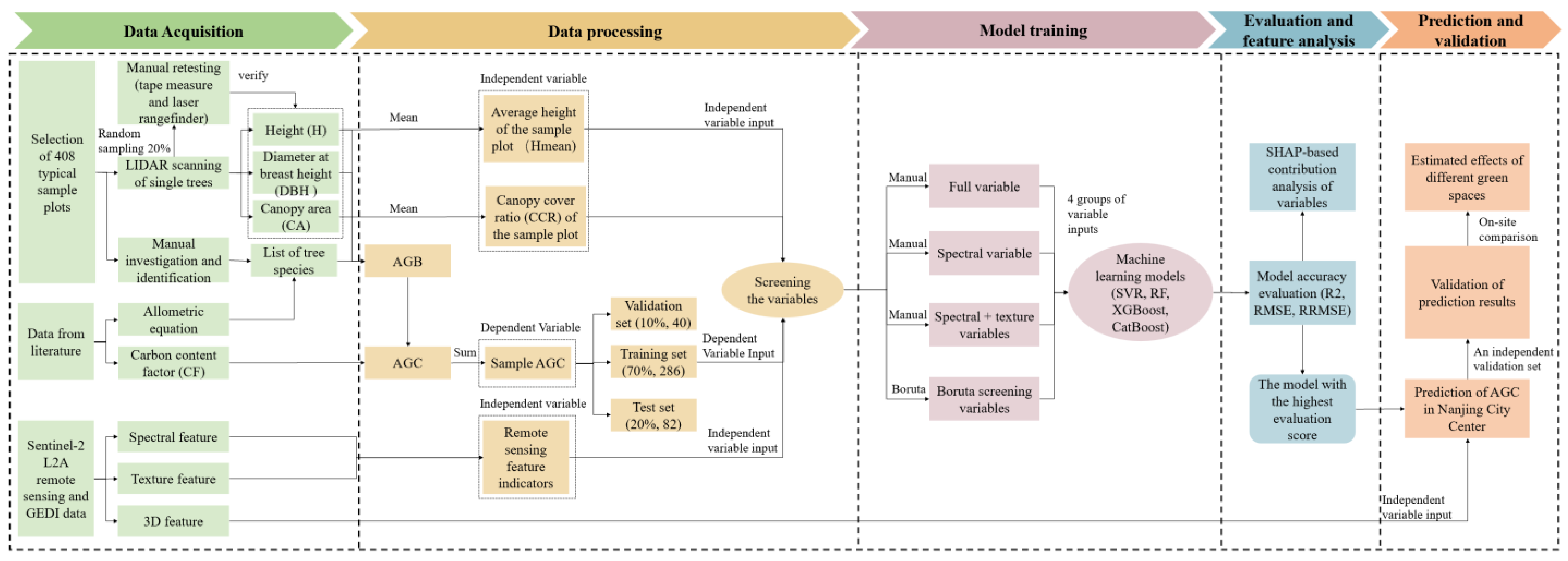
Figure 1. The research framework encompasses data acquisition, data processing, model training, model evaluation, feature analysis, prediction, and validation.
Forests 16 01381 g001
Figure 2. Study area and sampling plot distribution (The red line represents the central urban area of Nanjing and the boundaries of its districts, and the blue line represents the Yangtze River).
Forests 16 01381 g002
Figure 3. Tree-based importance (blue) reflects each feature’s contribution during model splits, while permutation importance (orange) indicates the impact on model performance when the feature is randomly permuted; features include structural (Hmean, CCR), spectral (B2–B5, B12), and vegetation indices (NDVI, RVI, DVI).
Forests 16 01381 g003
Figure 4. Correlation matrix of structural, spectral, and vegetation index features; ellipse orientation and color indicate correlation direction (left-tilted/orange = positive, right-tilted/blue = negative), while ellipse narrowness and color intensity reflect correlation strength (narrower and darker = stronger). Values without asterisks are not significant (p ≥ 0.05). ** indicate significance at 0.01 levels.
Forests 16 01381 g004
Figure 5. Comparison of evaluation indicators for four models, based on all variables.
Forests 16 01381 g005
Figure 6. Comparison of evaluation indicators for four models, based on spectral-variables.
Forests 16 01381 g006
Figure 7. Comparison of evaluation indicators for four models based on spectral + texture variables.
Forests 16 01381 g007
Figure 8. Comparison of evaluation indicators for four models based on Boruta screened variables.
Forests 16 01381 g008
Figure 9. SHAP summary chart.
Forests 16 01381 g009
Figure 10. Dependency graph of the top four variables.
Forests 16 01381 g010aForests 16 01381 g010b
Figure 11. Spatial distribution of AGC in Nanjing in 2024.
Forests 16 01381 g011
Table 1. Estimated effects of different green spaces.
Type of Green Space(a) Satellite RGB Imagery(b) Estimated Results
ParksForests 16 01381 i001Forests 16 01381 i002
RoadsForests 16 01381 i003Forests 16 01381 i004
ResidentialForests 16 01381 i005Forests 16 01381 i006
CampusForests 16 01381 i007Forests 16 01381 i008
LegendForests 16 01381 i009
Disclaimer/Publisher’s Note: The statements, opinions and data contained in all publications are solely those of the individual author(s) and contributor(s) and not of MDPI and/or the editor(s). MDPI and/or the editor(s) disclaim responsibility for any injury to people or property resulting from any ideas, methods, instructions or products referred to in the content.