Author Contributions
Conceptualization, Y.-X.L. and W.-X.Z.; methodology, Y.-X.L. and W.-X.Z.; software, Y.-X.L. and P.H.; validation, Y.-X.L.; formal analysis, Y.-X.L.; investigation, Y.-X.L.; resources, W.-X.Z.; data curation, Y.-X.L.; writing—original draft preparation, Y.-X.L.; writing—review and editing, W.M., W.-X.Z. and Y.-X.L.; visualization, Y.-X.L.; supervision, W.-X.Z.; project administration, W.-X.Z.; funding acquisition, W.-X.Z. All authors have read and agreed to the published version of the manuscript.
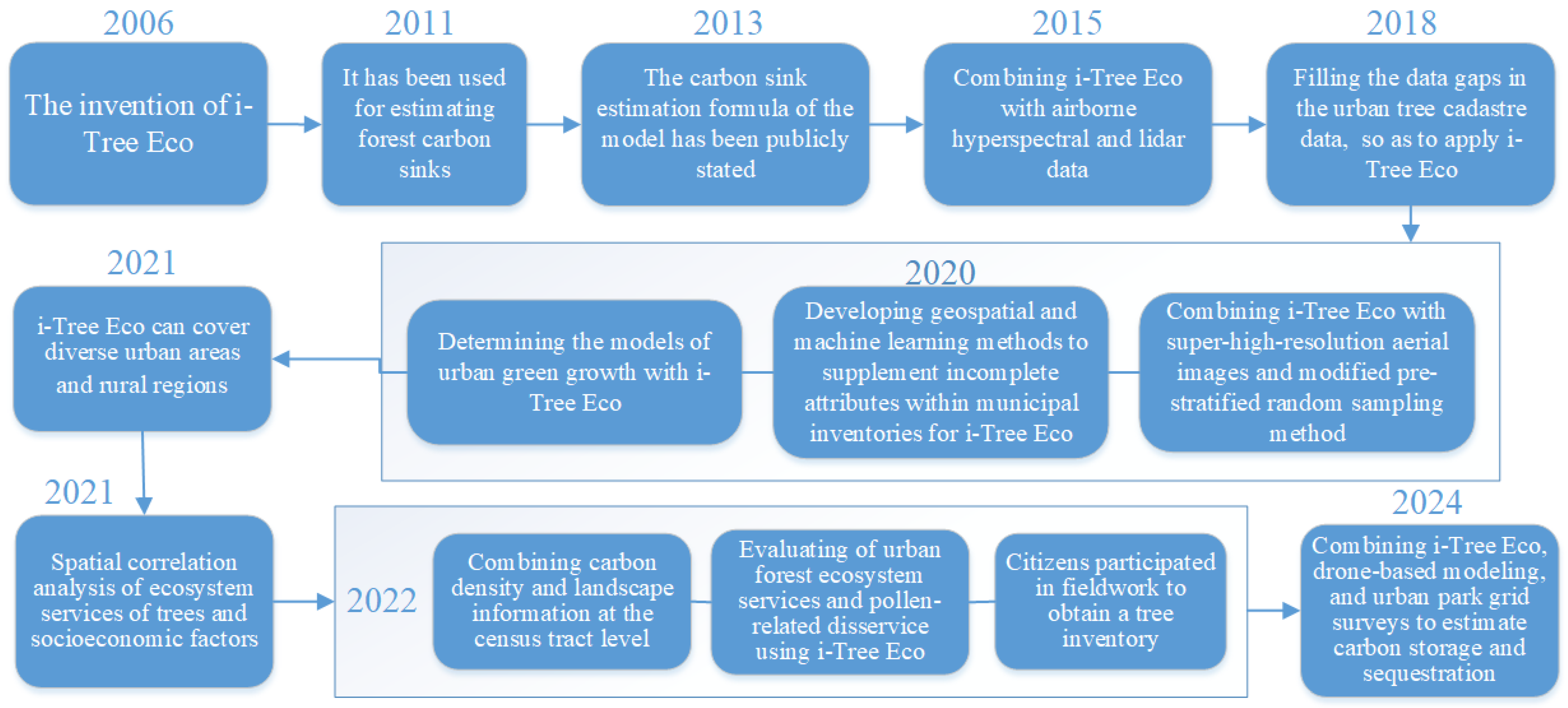
Figure 1.
Timeline of the development of i-Tree Eco for carbon sink estimation [
8,
20,
21,
22,
26,
28,
30,
34,
35,
36,
37,
38,
39].
Figure 1.
Timeline of the development of i-Tree Eco for carbon sink estimation [
8,
20,
21,
22,
26,
28,
30,
34,
35,
36,
37,
38,
39].
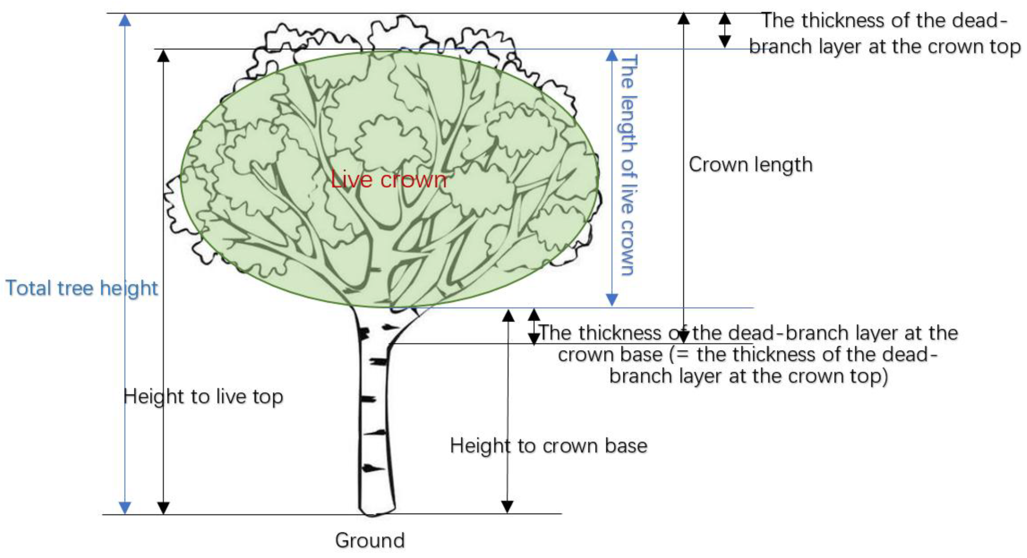
Figure 2.
Side view of a tree (with relevant indicators).
Figure 2.
Side view of a tree (with relevant indicators).
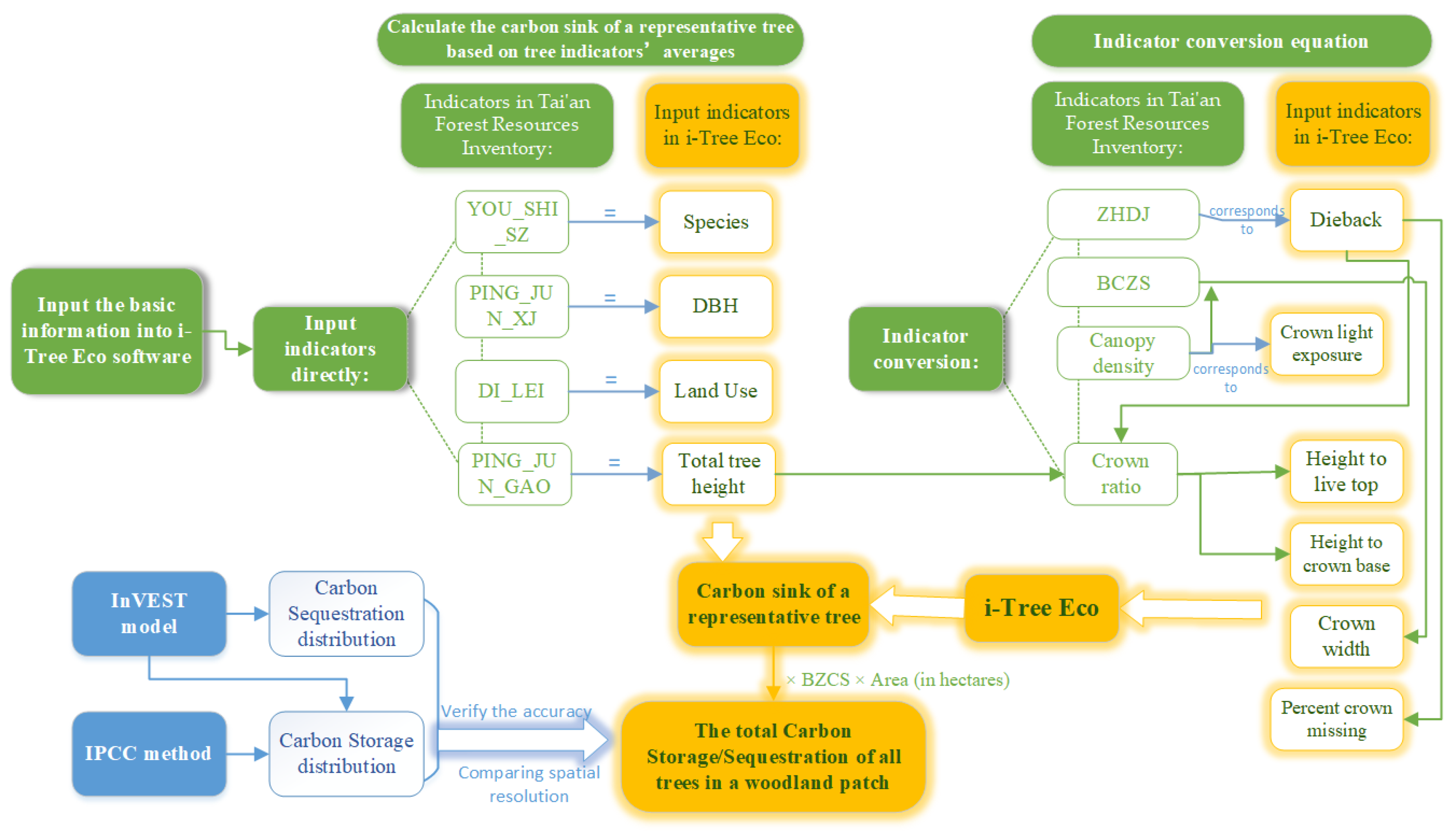
Figure 3.
Flowchart integrating the Tai’an Forest Resources Inventory data with i-Tree Eco in this study.
Figure 3.
Flowchart integrating the Tai’an Forest Resources Inventory data with i-Tree Eco in this study.
Figure 4.
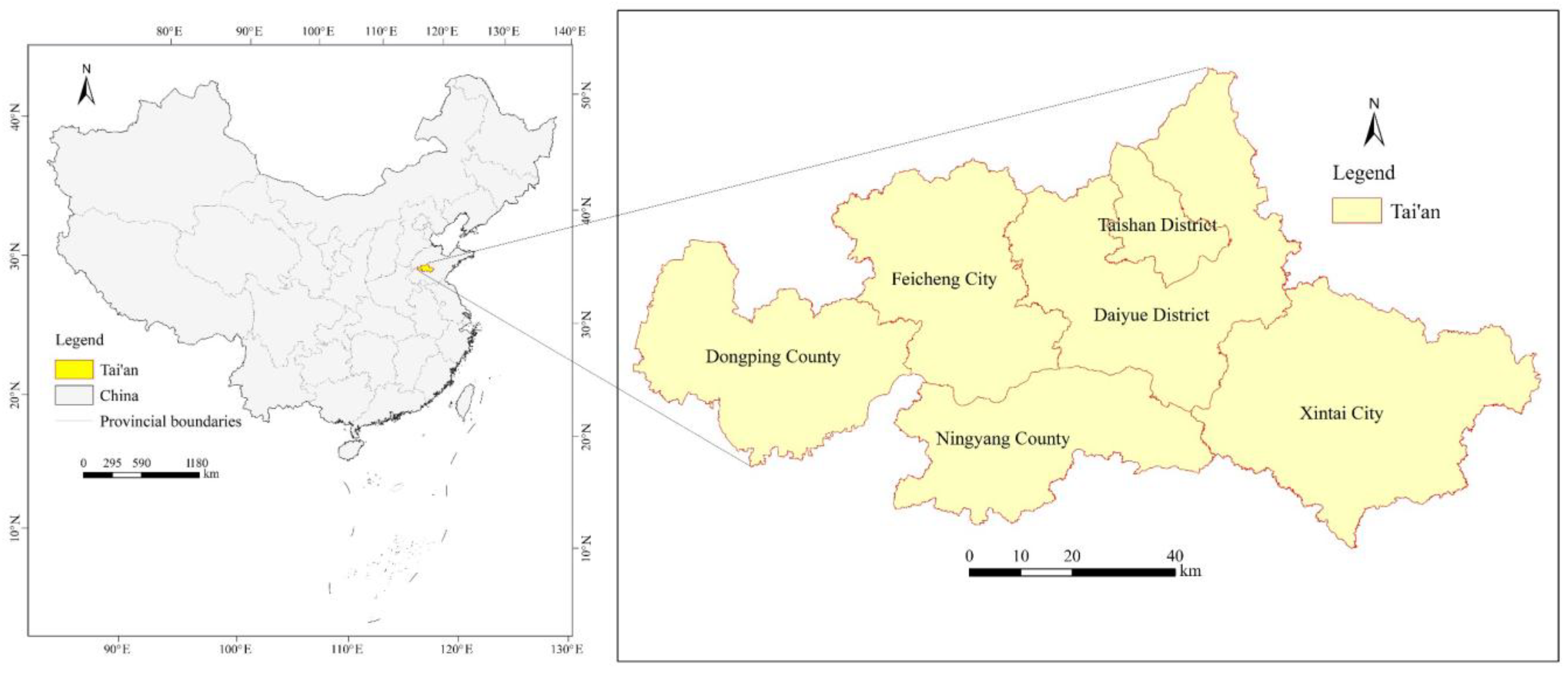
Location of Tai’an.
Figure 4.
Location of Tai’an.
Figure 5.
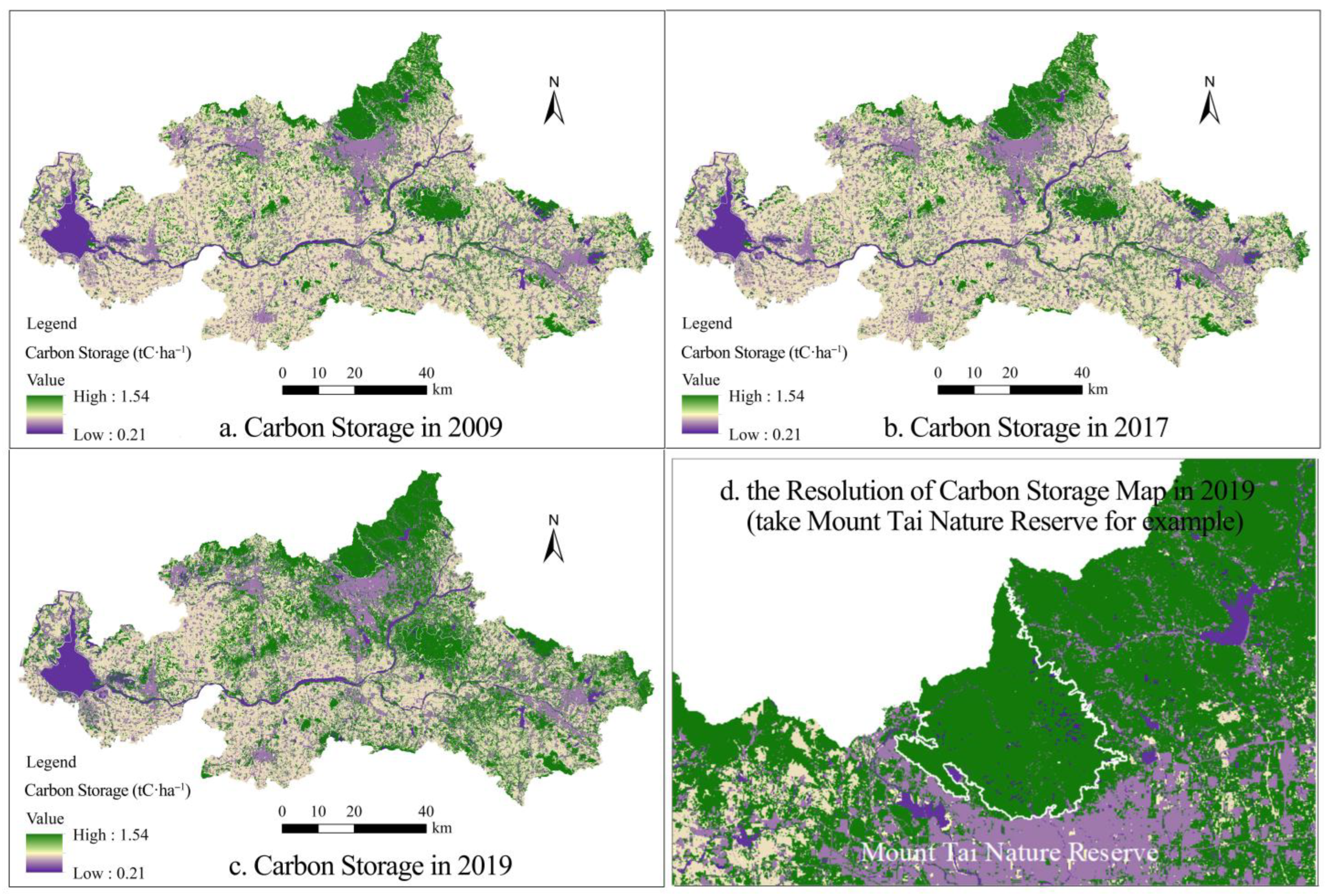
InVEST: Tai’an carbon storage. Notes: (a–d) show the carbon storage distribution obtained using the InVEST model. (a–c) are based on Tai’an’s Second National Land Survey data (2009), Tai’an’s Second National Land Survey—Change Survey data (2017), and Tai’an’s Third National Land Survey data (end of 2019), respectively. The figures demonstrate the distribution and changes in carbon storage throughout Tai’an in 2009, 2017, and 2019. (d) shows a localized, enlarged, and detailed view of (c) in order to illustrate the distribution of carbon storage in and around Mount Tai Nature Reserve. (d) highlights the clarity of the carbon storage distribution maps obtained by combining land use data with the carbon sink estimation method of the InVEST model, allowing the resolution of the InVEST method for estimating carbon sinks to be visualized.
Figure 6.
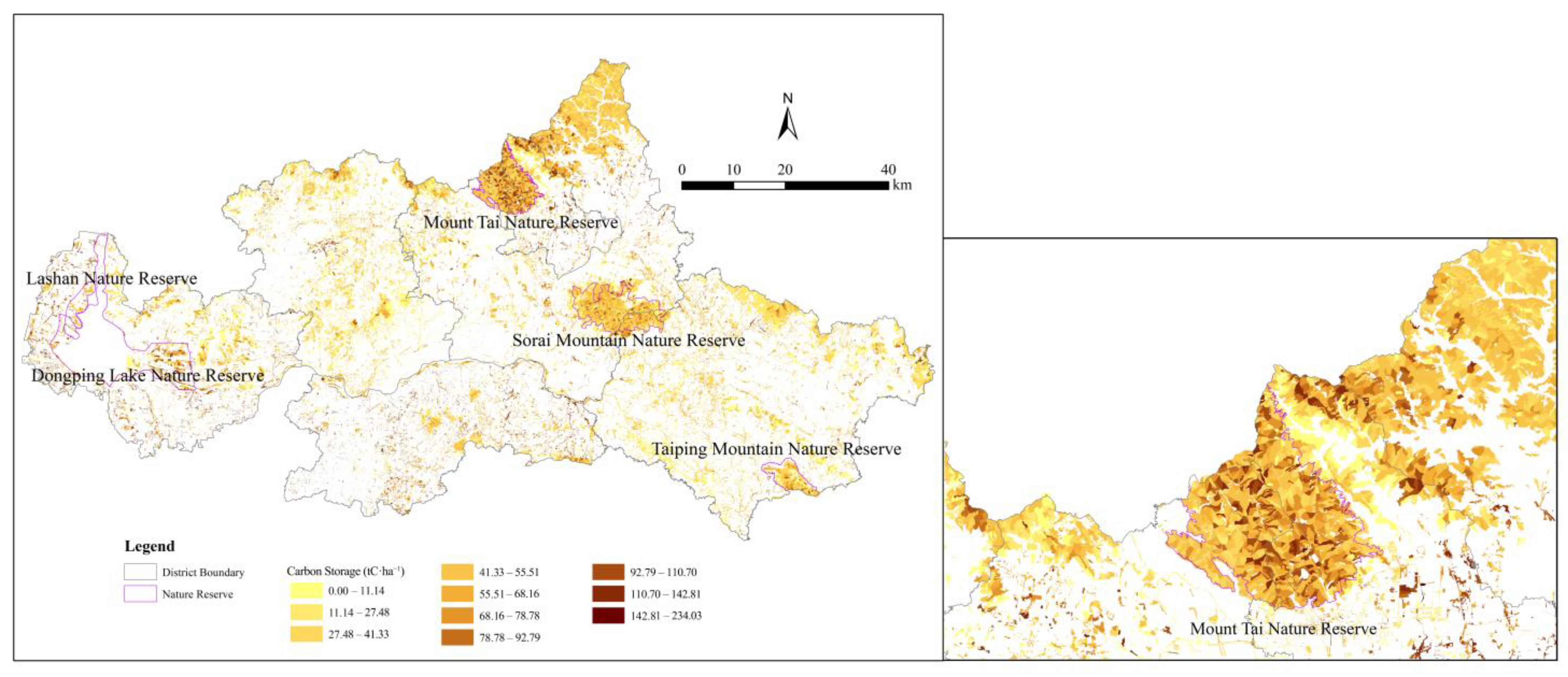
IPCC method: forest carbon storage in Tai’an in 2019 (unit: tC·ha−1). Note: This Figure shows the distribution of carbon storage in Tai’an City in 2019 obtained using the IPCC method, based on the Tai’an Forest Resources Inventory Geographic Information Database (2019). It demonstrates the distribution of carbon storage within the city’s woodlands. The figure on the right is a localized, enlarged, and detailed view of the figure on the left, showing the distribution of carbon storage in and around Mount Tai Nature Reserve. The figure on the right highlights the clarity of the carbon storage map obtained by combining the forest resources inventory with the IPCC method of estimating carbon sinks, allowing the resolution of the IPCC method for estimating carbon sinks to be visualized.
Figure 7.
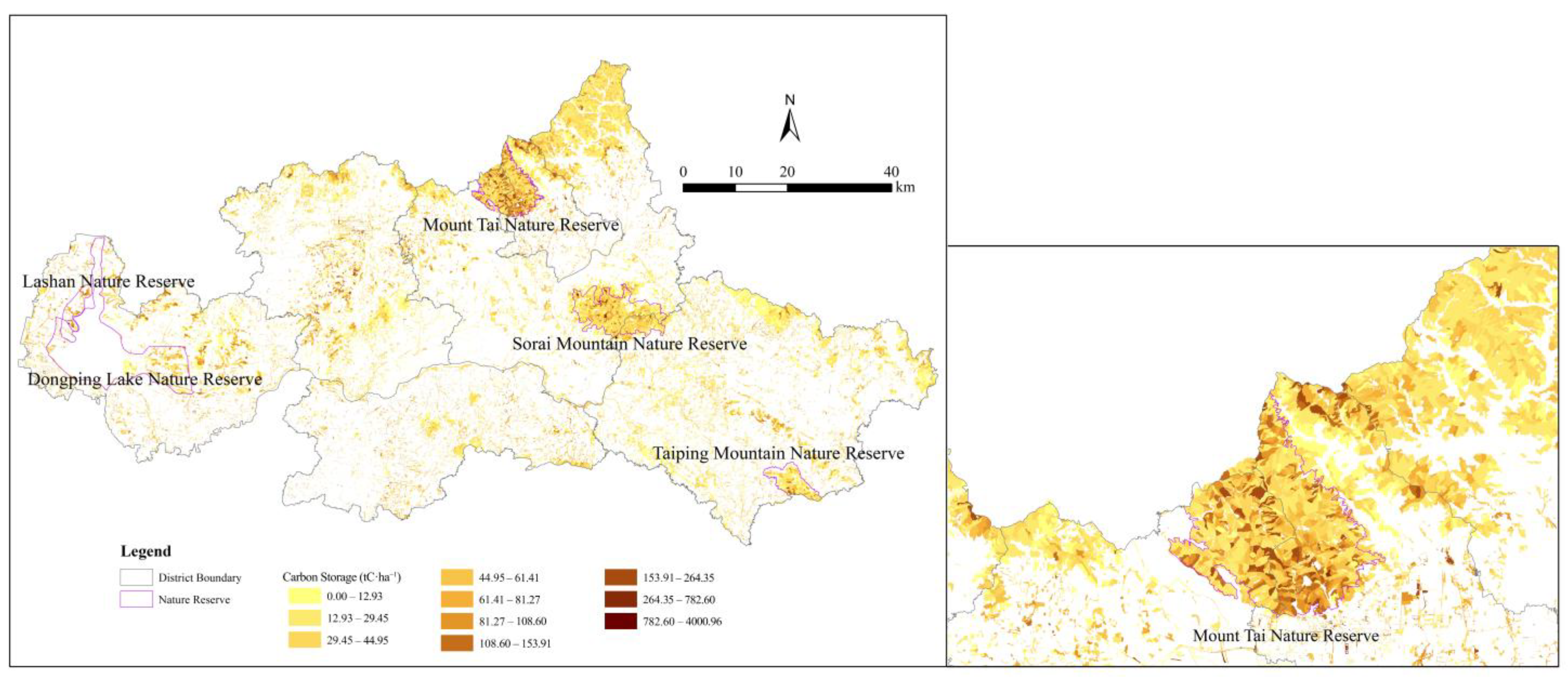
i-Tree Eco: forest carbon storage in Tai’an in 2019 (unit: tC·ha−1). Note: This Figure shows the distribution of carbon storage in Tai’an City in 2019 obtained using the i-Tree Eco method. It is based on the Tai’an Forest Resources Inventory Geographic Information Database (2019) and demonstrates the distribution of carbon storage within the city’s woodlands. The figure on the right is a localized, enlarged, and detailed view of the figure on the left, showing details of the distribution of carbon storage in and around Mount Tai Nature Reserve. The figure on the right shows the clarity of the carbon storage map obtained by combining the forest resources inventory with the i-Tree Eco model for carbon sink estimation, which allows the resolution of the i-Tree Eco model to estimate carbon sinks to be visualized.
Figure 8.
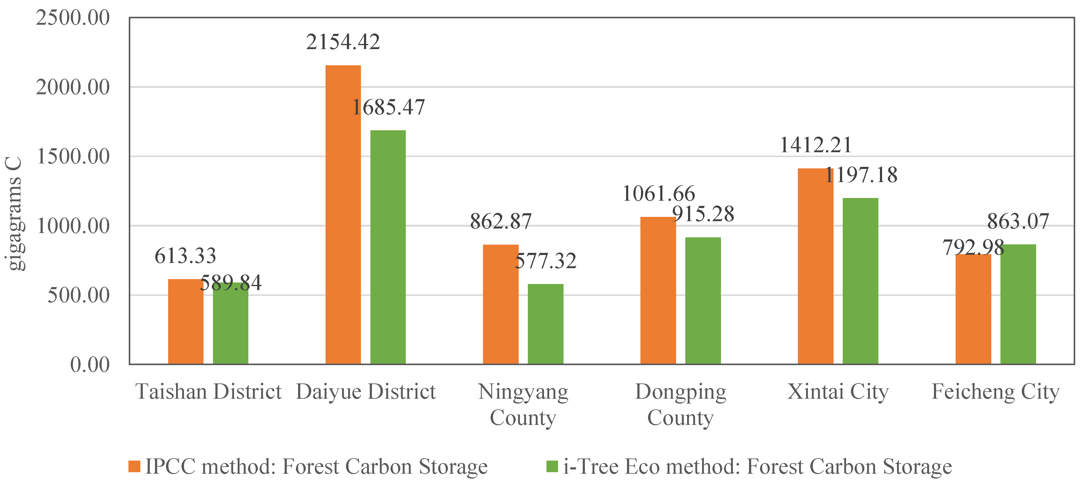
Forest carbon storage in Tai‘an’s districts and counties in 2019 using the IPCC method and the i-Tree Eco method.
Figure 8.
Forest carbon storage in Tai‘an’s districts and counties in 2019 using the IPCC method and the i-Tree Eco method.
Figure 9.
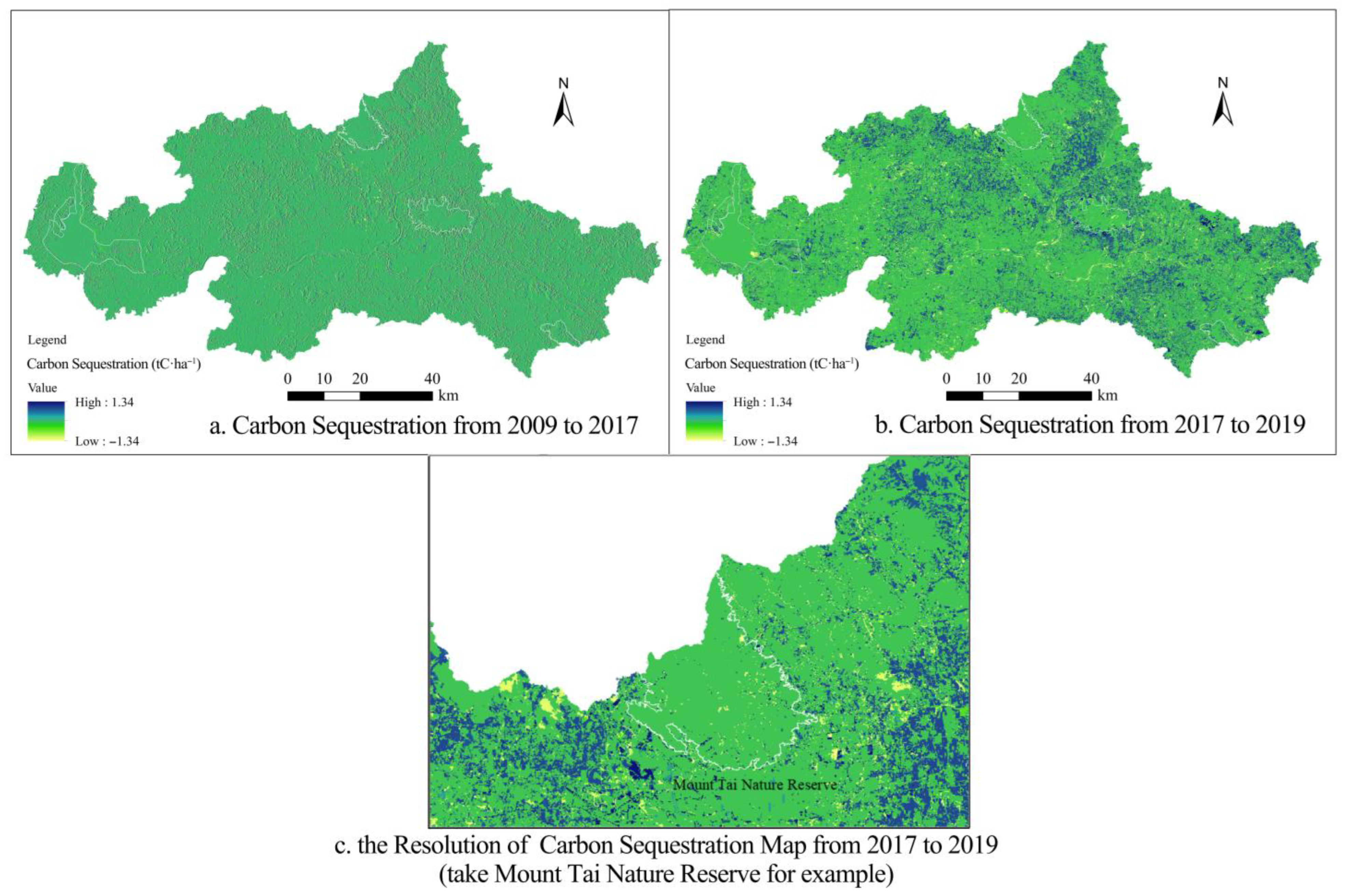
InVEST: carbon sequestration in Tai’an. Note: (a–c)show the distribution of carbon sequestration obtained using the InVEST model. (a,b) are based on the land use change between Tai’an’s Second National Land Survey data (2009) and Tai’an’s Second National Land Survey—Change Survey data (2017), as well as between Tai’an’s Second National Land Survey—Change Survey data (2017) and Tai’an’s Third National Land Survey data (end of 2019). (a,b) show the distribution of carbon sequestration in Tai’an for the years 2009–2017 and 2017–2019, respectively, showing the distribution of carbon sequestration throughout the city during the two periods. This part of the carbon sequestration is caused by land use change. (c) shows a localized, enlarged, and detailed view of (b) to demonstrate the details of the distribution of carbon sequestration in and around Mount Tai Nature Reserve. (c) shows the clarity of the carbon sequestration maps obtained by combining land use change data with the carbon sink estimation method of the InVEST model, allowing the resolution of the InVEST method for estimating carbon sinks to be visualized.
![Forests 16 01363 g009 Forests 16 01363 g009]()
Figure 10.
i-Tree Eco: annual carbon sequestration of forests in Tai’an in 2019. Note: This Figure shows the distribution of carbon sequestration in Tai’an City in 2019 obtained using the i-Tree Eco method. It is based on the Tai’an Forest Resources Inventory Geographic Information Database (2019), demonstrating the distribution of carbon sequestration across the city’s forests. This part of carbon sequestration is caused by CO2 uptake by existing tree growth. The figure on the right is a localized, enlarged, and detailed view of the figure on the left, showing details of the distribution of carbon sequestration in and around Mount Tai Nature Reserve. The figure on the right highlights the clarity of the carbon sequestration map obtained by combining forest resources inventory data with the i-Tree Eco model. The resolution of the i-Tree Eco model for estimating carbon sinks can be visualized.
Figure 11.
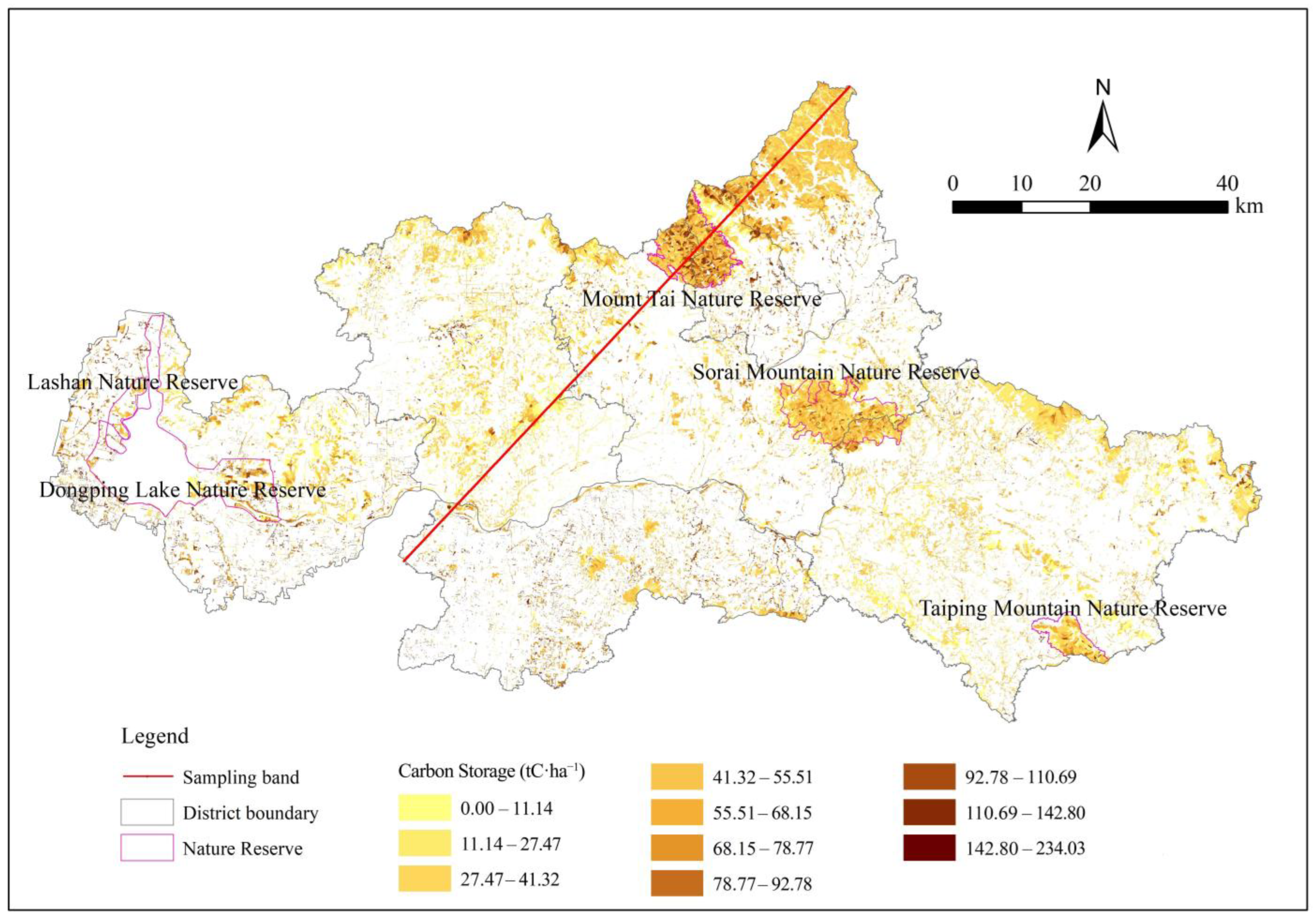
Schematic diagram of the sampling band location.
Figure 11.
Schematic diagram of the sampling band location.
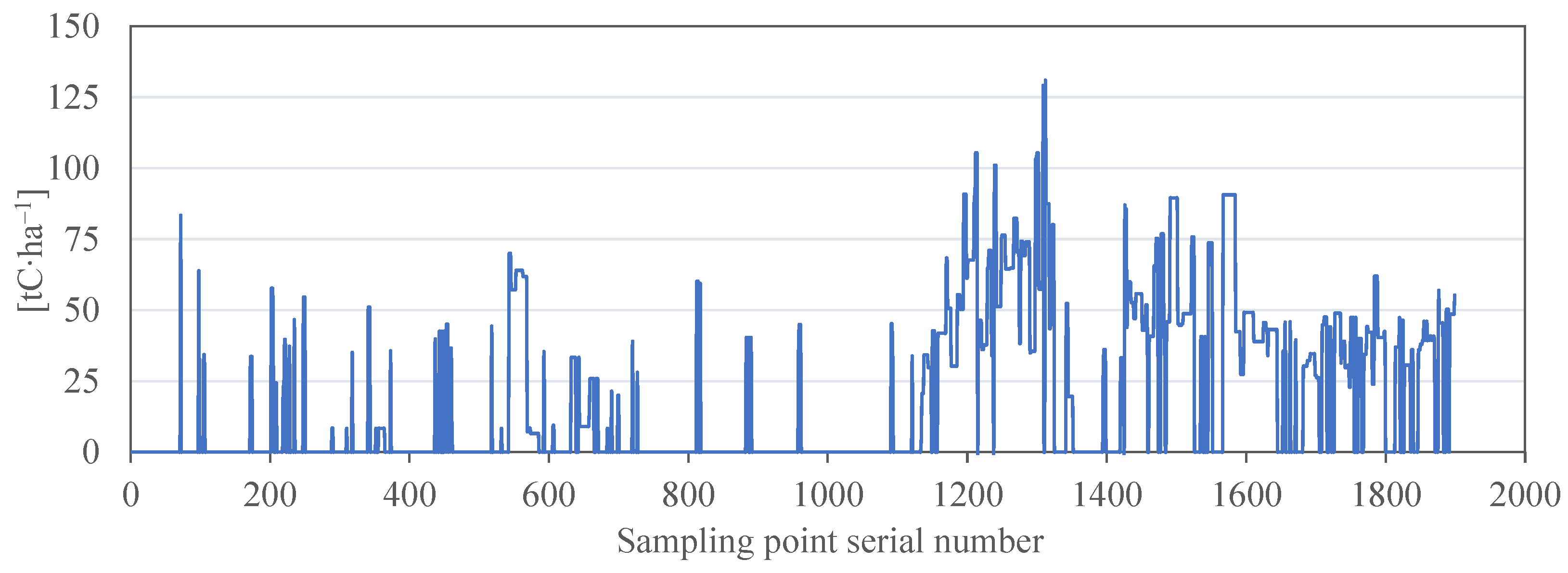
Figure 12.
InVEST calculation of carbon storage density sampling band values of 2019. Note: The figure shows the series of values taken from the intersection of the sampling band with the distribution map of carbon storage density in Tai’an City in 2019, which were obtained using the InVEST method.
Figure 12.
InVEST calculation of carbon storage density sampling band values of 2019. Note: The figure shows the series of values taken from the intersection of the sampling band with the distribution map of carbon storage density in Tai’an City in 2019, which were obtained using the InVEST method.
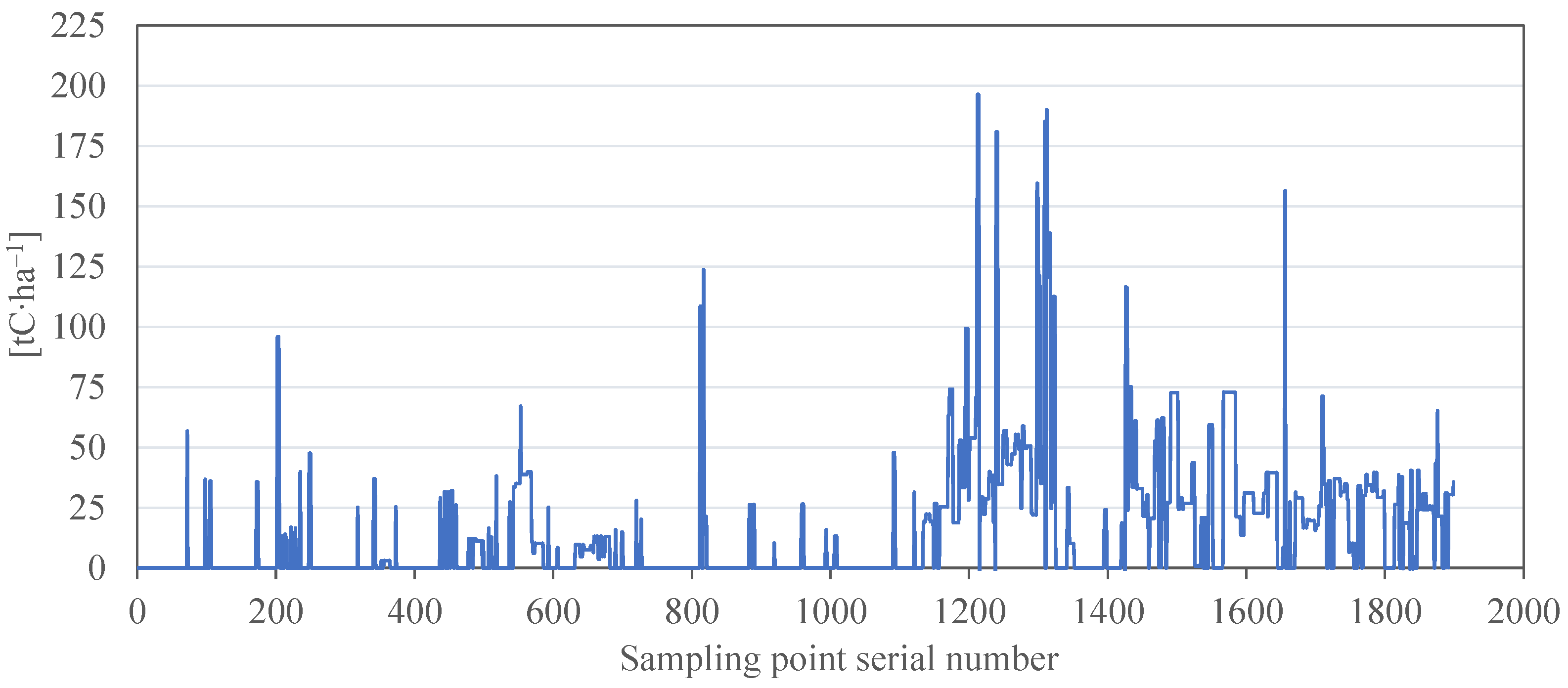
Figure 13.
IPCC method calculation of carbon storage density sampling band values of 2019. Note: The figure shows the series of values taken from the intersection of the sampling band with the distribution map of carbon storage density in Tai’an City in 2019, which were obtained using the IPCC method.
Figure 14.
i-Tree Eco calculation of carbon storage density sampling band values for 2019. Note: The figure shows the series of values taken from the intersection of the sampling band with the distribution map of carbon storage density in Tai’an City in 2019, which were obtained using the i-Tree Eco method.
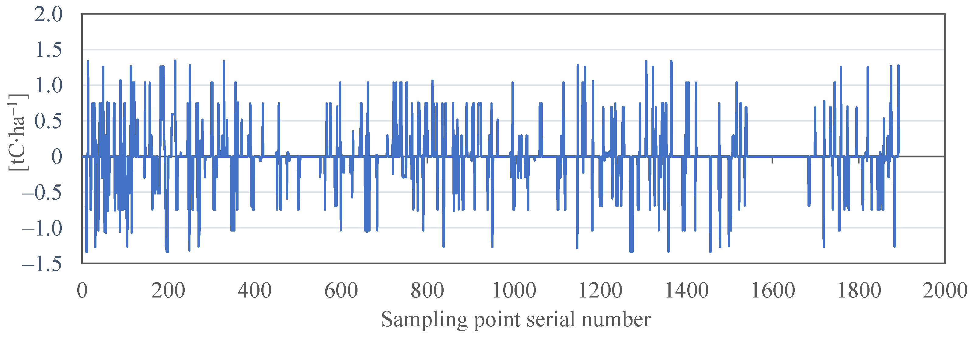
Figure 15.
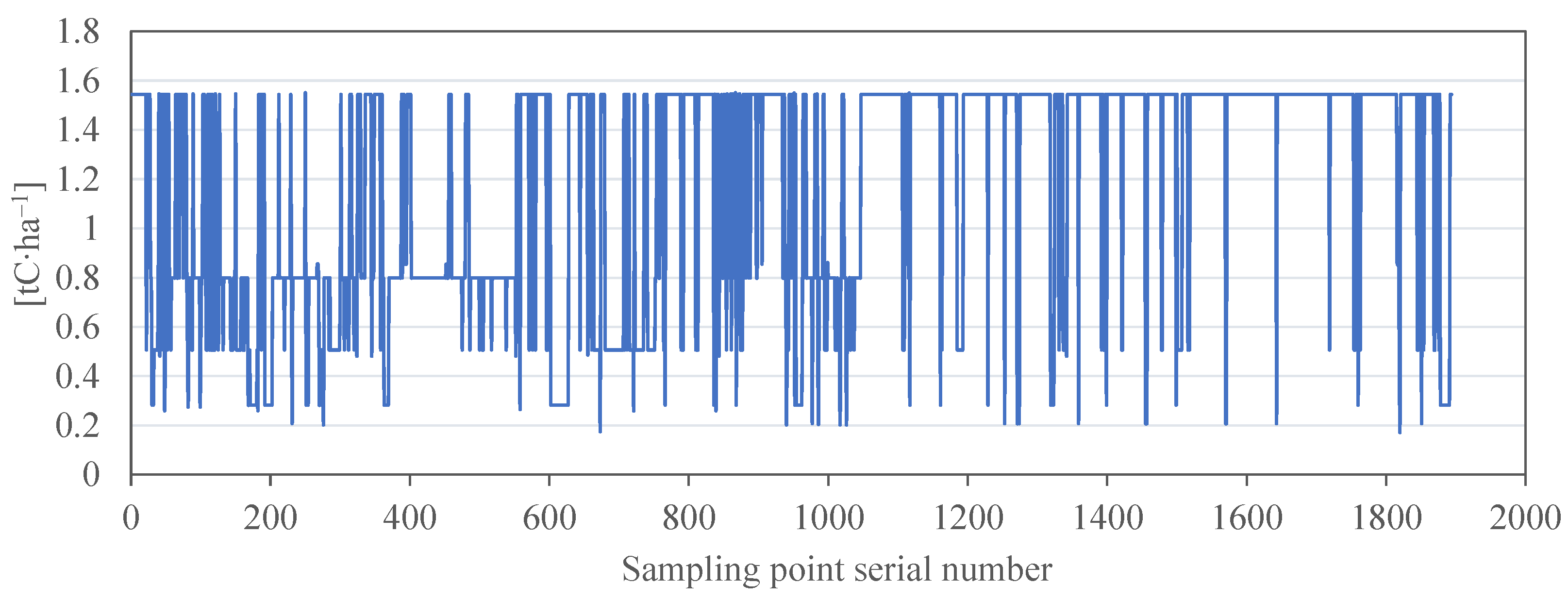
Values of the sampling band calculated using InVEST for the carbon sequestration density from 2009 to 2017. Note: The figure shows the series of values taken from the intersection of the sampling band with the distribution map of carbon sequestration density in Tai’an City between 2009 and 2017, which were obtained using the InVEST method.
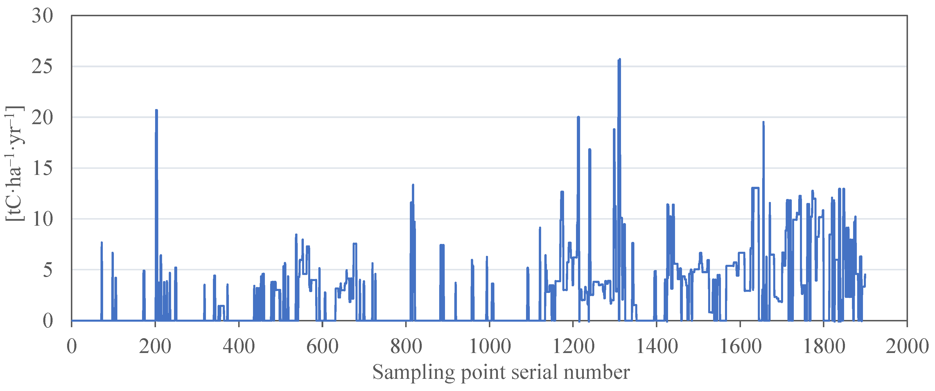
Figure 16.
Values of the sampling band calculated using i-Tree Eco for the carbon sequestration density in 2019. Note: The figure shows the series of values taken from the intersection of the sampling band with the distribution map of carbon sequestration density in Tai’an City in 2019, which were obtained using the i-Tree Eco method.
Table 1.
Advantages and disadvantages of current carbon sink estimation models.
Table 1.
Advantages and disadvantages of current carbon sink estimation models.
| Models | Applicable Scale | Advantages | Shortcomings of Carbon Sink Estimation Models at the Small Scale and for Green Space Planning and Management |
|---|
| ➀ Sample plot inventory–sample marking tree analysis | Individual plant scale [10] | The method is clear and technology is simple [11], directly measures biomass, and is accurate [10]. | The inventory investigating workload is heavy; does not take all types of terrestrial ecosystem into account; carbon sinks are calculated based on the annual change in carbon storage, making the carbon sink estimation error larger [11]. |
| Empirical model simulation method |
| ➁ Tree allometric growth equation (i-Tree Eco model) | Individual plant scale and regional scale | Calculations with the tree allometric growth equation method are quick [10]. i-Tree Eco estimates carbon sequestration and carbon storage of forests based on the different growth rates of different tree species, DBH (diameter at breast height), and total heights. | Direct calculation using the allometric growth equation requires a large amount of measured data and the growth stages and regional differences in tree species must be considered [10]. i-Tree Eco also requires a large amount of inventory investigation work. Therefore, it can generally only be used for small-scale research. It does not consider other ecosystem types. |
| ➂ CITYgreen | City and regional scale/park and community scale [12] | Regional-scale analysis is quick. Park- and community-scale analysis can be used to estimate individual trees without requiring remote sensing images [12]. | Regional-scale analysis requires image pre-classification; there is uncertainty in the estimation results [13,14]. Park- and community-scale analyses are small in scope, require digitization, and are time-consuming [12]; the input attributes require sample plot inventory [15]; it is mainly used in artificial forests [15]. |
| ➃ InVEST | Regional scale | The operation is simple, input data are easy to obtain, and it can cover various ecosystem types. | The internal heterogeneity of forest carbon density is not considered; attribute modifications are needed based on local conditions [10]; does not consider the carbon sequestration effect of the natural growth of trees. |
| Mechanism model simulation methods |
| ➄ CENTURY model (belongs to the static model class) | Regional scale [17] | It is a carbon element simulation model based on the structure and function of soil [17]. | Lack of refined simulation of the photosynthesis process [17]. |
| ➅ IBIS model (belongs to the dynamic model class) | Regional scale [17] | It comprehensively considers geochemical, geophysical, and vegetation dynamic processes. It is often used to simulate complex carbon cycle processes [17]. | The large number of different types of attributes required limits its wider application [17]. |
| ➆ LPJ-GUESS model (belongs to the dynamic model class) | From species to global scales [17] | It can simulate the structure and function of forest ecosystems at multiple scales including individual species [17,23,24]. | The model code is complex; vegetation and soil type data with high spatial resolution must be input; to obtain regional data, extensive field plot surveys or interpolations based on flux site data are needed; attribute adjustment takes a long time [16]. |
Table 2.
Innovative applications and method optimizations of i-Tree Eco in urban studies.
Table 2.
Innovative applications and method optimizations of i-Tree Eco in urban studies.
| Number | Research Area | Research Topic | Data Prepared in Advance | Analysis Method |
|---|
| 1 [21] | Santa Barbara, California, United States | Urban forest ecosystem services | Fusion of hyperspectral imagery; waveform radar data | Discriminant analysis method for the tree crown scale—fusion airborne visible light and infrared imaging spectroscopy; laser radar structure measurement; estimating leaf area index using laser penetration and allometric measurement methods |
| 2 [8] | New York, United States | Urbanization and the relationship between canopy coverage morphology and carbon density | High-resolution land cover map; laser radar-derived tree index; fieldwork data | Radar measurement; aggregate carbon density and landscape information at the census tract level; R statistical analysis |
| 3 [19] | A park in Munich, Germany | i-Tree Eco model’s simulation of light sensitivity and tree species classification; development of a remote sensing observation method for crown light exposure (CLE) | Detailed inventory data of the forest | An automated method combined with remote sensing to calculate the CLE based on tree and crown morphology; assesses how ecosystem services and disservices are altered when the degree of species and CLE detail diminishes |
| 4 [38] | Chicopee and Fall River, Massachusetts, United States | Value and distribution of energy savings provided by saplings; value changes in the future | The inventory of 2271 saplings on the streets or in residential areas planted from 2014 to 2015 | Spatial correlation analysis of ecosystem services of saplings and socioeconomic factors in census tracts; spatial correlation analysis of forest ecological characteristics and the ecosystem services they provide |
| 5 [40] | Adama City, Ethiopia | Urban forest ecosystem services—effect on climate change mitigation | Investigation data from 214 sample plots | Leaf area/biomass of trees and shrubs, pollution removal, volatile organic compound emissions, hydrological function, forest ecosystem value, and carbon storage and sequestration were estimated; the structure and makeup of urban forests were investigated and analyzed |
| 6 [20] | Royal Forest of Capodimonte, Naples, Italy | Urban forest ecosystem services (ES) and pollen-related disservice assessment (ED) | Plant community survey and biodiversity value assessment | Analysis of ecosystem services and pollen disservices provided by urban forests through data spatialization; evaluation of ES and ED using i-Tree Eco and Index of Urban Green Zones Allergenicity (IUGZA) |
| 7 [22] | Oslo’s built-up areas, Norway | Filling in the missing and incomplete attributes for i-Tree Eco in current urban forest inventories, thereby enabling quick and low-cost estimation of urban ecosystems | Manual measurement, airborne laser scanning crown images, land use map, and land resource map | Using geospatial analytics and machine learning methods; manual measurement was correlated with airborne laser scanning crown images to complete the tree measurements, employing an ancillary spatial dataset to obtain the missing attributes of trees’ spatial background; machine learning with Bayesian networks was used to deduce the output of i-Tree Eco and infer the ecological value of citywide forest inventories |
| 8 [26] | Perugia, Italy | Citizens participated in fieldwork to obtain a tree inventory, assessing the ecosystem services offered by urban trees | Italian Urban Forest Inventory Dataset; public datasets on weather data, pollutant concentrations and urban morphology; urban greening data collected by citizens | A tool was designed to aid decision-making and management for tree planting; four ecosystem services offered by urban trees were assessed by i-Tree Eco |
Table 3.
Correspondence between the “disaster level” ZHDJ indicator and the dieback indicator, as derived from [
43]. NAFT refers to the number of affected forest trees. The dieback indicator is set to be equal to the average tree damage severity.
Table 3.
Correspondence between the “disaster level” ZHDJ indicator and the dieback indicator, as derived from [
43]. NAFT refers to the number of affected forest trees. The dieback indicator is set to be equal to the average tree damage severity.
| “Disaster Level” ZHDJ Indicator [43] | Disaster Types: Forest Pests and Diseases | Disaster Types: Forest Fire | Disaster Types: Climate Damage and Others |
|---|
| Evaluation Standard [43] | Average Tree Damage Severity | Evaluation Standard [43] | Average Tree Damage Severity | Evaluation Standard [43] | Average Tree Damage Severity |
|---|
| 0 (approximate to zero) | NAFT is less than 10% | 10% | No notable damage | 5% | No notable damage | 5% |
| 1. Light | NAFT is 10–29% | 20% | NAFT is less than 20%; still able to resume growth | 10% | NAFT is less than 20% | 10% |
| 2. Medium | NAFT is 30–59% | 44% | NAFT is 20–49%; growth is significantly inhibited | 40% | NAFT is 20–59% | 44% |
| 3. Severe | NAFT is more than 60% | 80% | NAFT is more than 50%, comprising mainly dying and dead wood | 80% | NAFT is more than 60% | 80% |
Table 4.
Correspondence between the “canopy density” indicator and the crown light exposure indicator, as derived from [
45].
Table 4.
Correspondence between the “canopy density” indicator and the crown light exposure indicator, as derived from [
45].
| Canopy Density | Crown light Exposure |
|---|
| ≥0.80 | 1 |
| 0.6–0.8 (including 0.6) | 2 |
| 0.34–0.6 (including 0.3) | 3 |
| 0.1–0.3 (including 0.1) | 4 |
| 0–0.1 (not including 0.1) | 5 |
Table 5.
Key variables of the i-Tree Eco model.
Table 5.
Key variables of the i-Tree Eco model.
| Indicator Name | Corresponding to Tai’an Forest Resources Inventory Attribute Table Code or Indicator Conversion Equation | Quantity Unit | Interpretation (i-Tree Software Interface Notes) [25] |
|---|
| Species | YOU_SHI_SZ (means dominant tree species) | | The names of the species and genus of each tree were identified and documented |
| DBH | PING_JUN_XJ (means the average of DBH) | cm | Precise measurement or categories of the DBH of the stem for each individual tree |
| Land Use | DI_LEI (means land type) | | The land use type where the tree is situated |
| Total tree height | PING_JUN_GAO (means the average of tree height) | m | The height from the ground to the uppermost part (whether alive or dead) of the tree |
| Crown size | Height to live top | Height to live top = Total tree height-Total tree height × CR ×(Dieback/100) | m | The height from the ground to the living top of the tree |
| Height to crown base | Height to crown base = Total tree height − Total tree height × CR × (1 –Dieback/100) | m | The height from the ground to the bottom of the living crown of the tree |
| Crown width | 2 × SQRT ((1 hectare × canopy density/BCZS)/π) | m | The crown width in two directions, namely north–south and east–west |
| Percent crown missing | Percent crown missing = 39.6 × (1 + Dieback/100) | Percentage of the crown volume that is unoccupied by branches and leaves |
| Crown health | Dieback | ZHDJ corresponds to the percentage of disease, as shown in Table 3 [43] | % | An estimation of the percentage of the crown that consists of dead branches |
| Crown light exposure | Enter crown light exposure according to canopy density; correspondence is shown in Table 4 [45] | | The number of tree sides that receive sunlight from above (maximum of 5) |
Table 6.
Input carbon pool values (tC·ha−1).
Table 6.
Input carbon pool values (tC·ha−1).
| Lucode | LULC_Name | C_above | C_below | C_soil | C_dead |
|---|
| 112 | Cropland | 7.05 | 6.64 | 65.76 | 0.43 |
| 222 | Woodland | 31.38 | 17.28 | 101.89 | 3.81 |
| 333 | Grassland | 7.44 | 11.56 | 63.93 | 2.57 |
| 444 | Water area | 0.74 | 0.37 | 26.81 | 0.32 |
| 555 | Built-up land | 2.88 | 1.58 | 45.96 | 0.21 |
| 666 | Unused land | 1.56 | 2.66 | 16.34 | 0.18 |
Table 7.
Forest carbon sequestration in Tai ‘an’s districts and counties in 2019 using the i-Tree Eco method.
Table 7.
Forest carbon sequestration in Tai ‘an’s districts and counties in 2019 using the i-Tree Eco method.
| District and County | i-Tree Eco Method: Forest Carbon Sequestration (tC·yr−1) |
|---|
| Taishan District | 68,556.02 |
| Daiyue District | 290,100.30 |
| Ningyang County | 91,263.49 |
| Dongping County | 124,533.00 |
| Xintai City | 214,052.74 |
| Feicheng City | 148,283.49 |
| Sum | 936,789.03 |
Table 8.
Regression model coefficients a,b.
Table 8.
Regression model coefficients a,b.
| Model | Non-Standardized Coefficient | Standardized Coefficient | t | Significance |
|---|
| B | Standard Error | Beta |
|---|
| i-Tree Eco method Carbon Storage | 1.002 | 0.003 | 0.905 | 400.254 | 0.000 |
Table 9.
Model summary c,d.
Table 9.
Model summary c,d.
| R | R2 b | Adjusted R2 | Error of Standard Estimation |
|---|
| 0.905 a | 0.820 | 0.820 | 147.099 |
