Acknowledgments
The authors gratefully acknowledge the following contributors for providing the images used in this study: Elisabeth Wheeler (North Carolina State University) for images from specimens BWCw 8556, BWCw 8332, BWCw 8618, BWCw 8516, PACw En.cyl, USw PR19, Hw 23557, BWCw 8058, FHOw 19992, and PACw 4673 (permission granted on 5 August 2025); Hans Beeckman (Royal Museum for Central Africa) for images from specimens Tw 17698, Tw 425, Tw 609, Tw 724, Tw 5225, Tw 6987, Tw 26885, Tw 52896, and Tw 5016 (permission granted on 12 August 2025); Peter Gasson (Royal Botanic Gardens, Kew) for images from specimens Kw Per.ela.Trade.1951, Kw Swi.mac, Kw 4353, Kw 70560, and FHOw 4291 (permission granted on 6 August 2025).
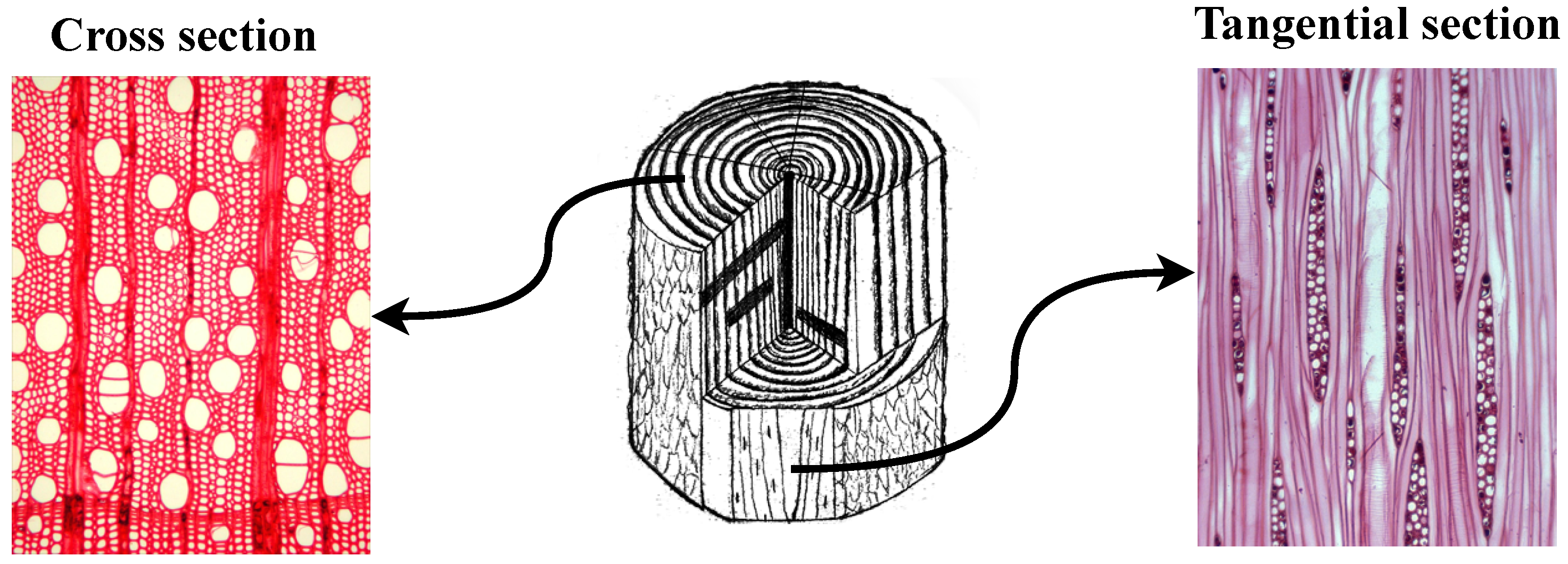
Figure 1.
Anatomical image positions in wood samples using Acer rubrum as an example. The left image (specimen BWCw 8556) shows the cross section (perpendicular to the growth rings), where vessels and parenchyma are visible; the right image (specimen BWCw 8332) shows the tangential section (parallel to the growth rings), where wood rays can be seen.
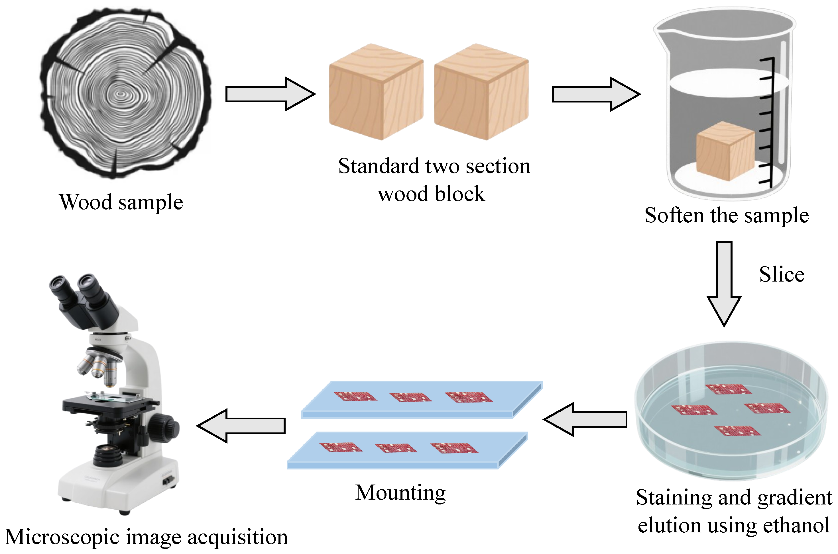
Figure 2.
Workflow of wood microscopic image acquisition. The steps of wood microscopic image acquisition include softening, slicing, staining, and mounting, then image capture using a Leica DM2000 LED microscope.
Figure 2.
Workflow of wood microscopic image acquisition. The steps of wood microscopic image acquisition include softening, slicing, staining, and mounting, then image capture using a Leica DM2000 LED microscope.
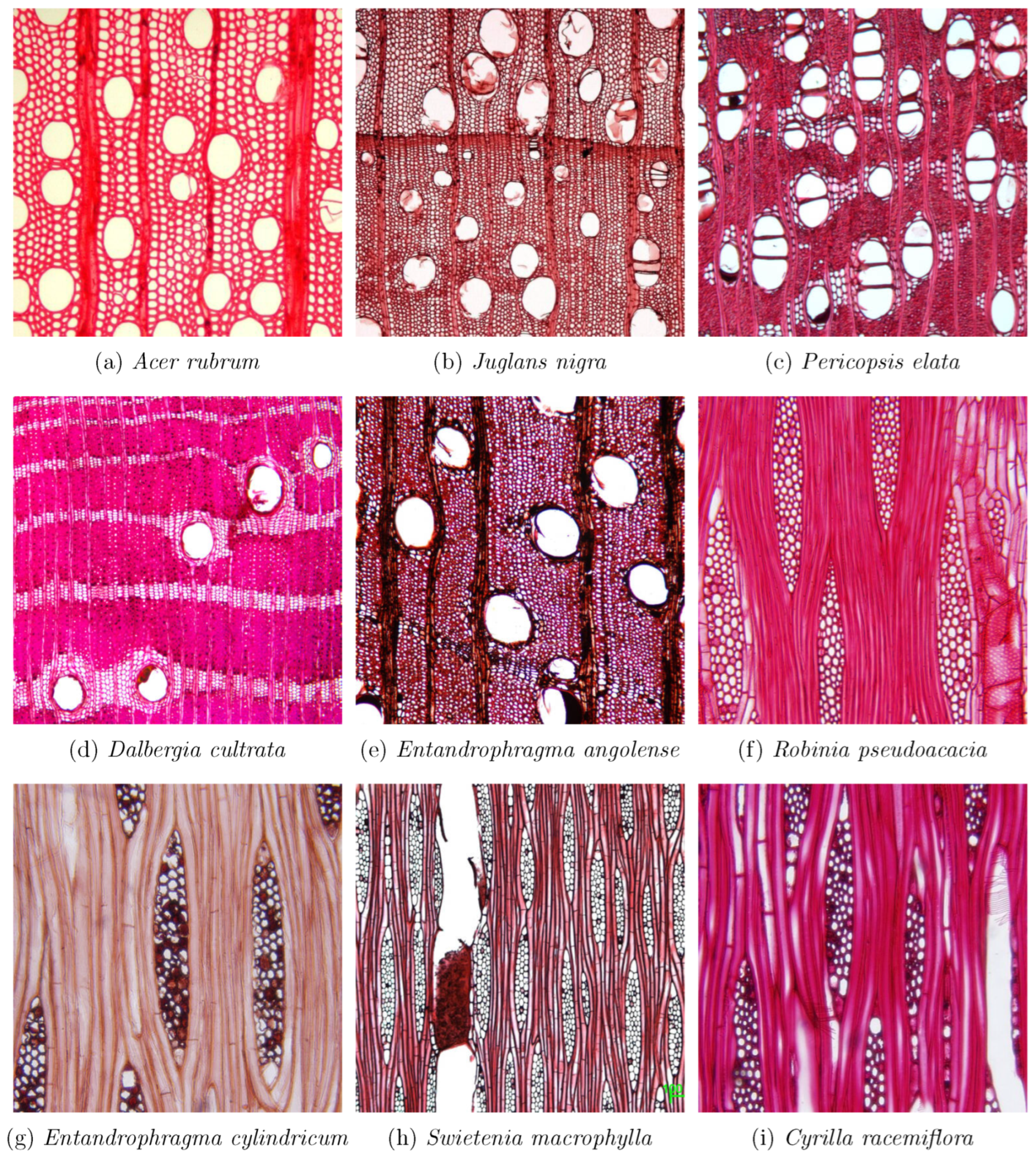
Figure 3.
Example images in the wood sections dataset. Subfigures (a–e) show cross-section images, where vessels and parenchyma are visible; Subfigures (f–i) show tangential section images, where wood rays are visible. Images from specimens: (a) specimen BWCw 8556, (b) specimen BWCw 8618, (c) specimen Kw Per.ela.Trade.1951, (e) specimen PACw 4673, (f) specimen BWCw 8516, (g) specimen PACw En.cyl, (h) specimen Kw Swi.mac, (i) specimen USw PR19.
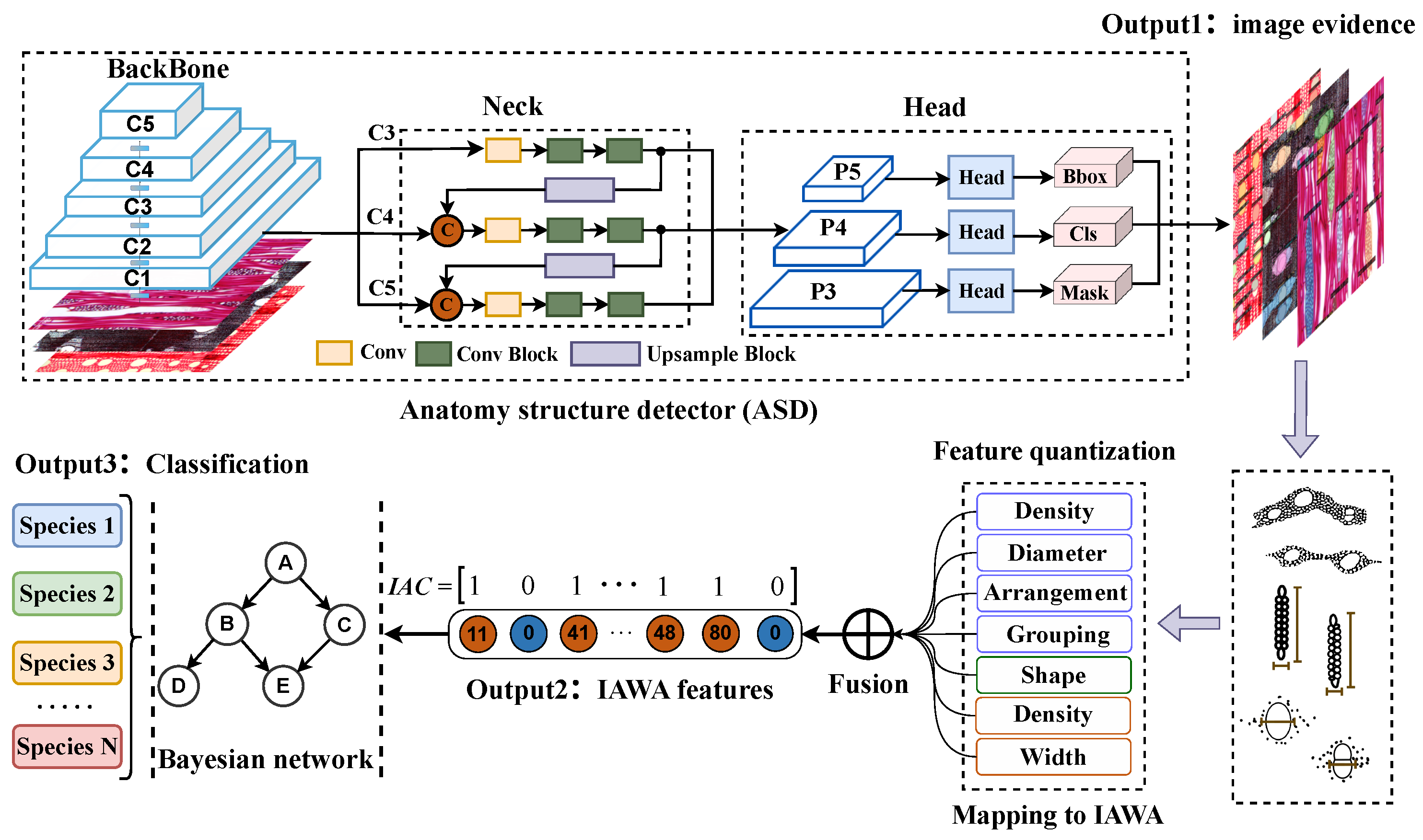
Figure 4.
Interpretable wood recognition process. The wood recognition method involves three steps: anatomical feature detection using an anatomy structure detector, quantifying features and mapping them to IAWA codes, and wood species identification using a Bayesian network. Example images from specimens: BWCw 8556, Kw 70560, and USw PR19.
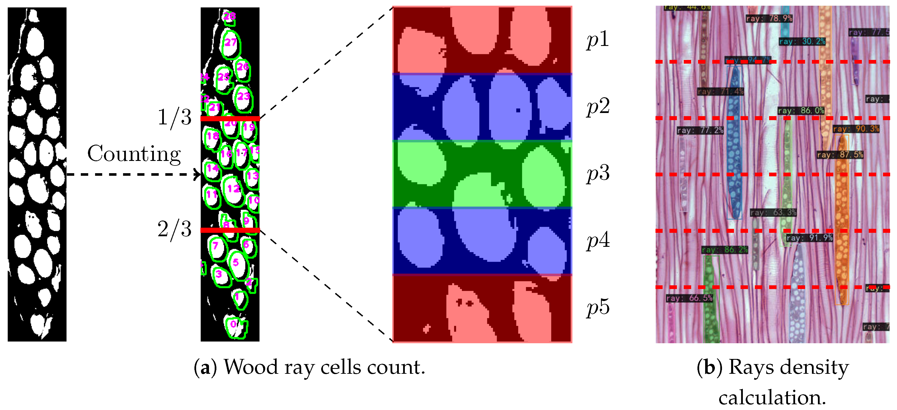
Figure 5.
Principle of the wood ray cells count and rays density calculation. (a) The middle area of the ray is divided into multiple parts. Count the number of cells in each part and calculate the average. (b) Divide the image (specimen BWCw 8332) into n equal horizontal sections and count the wood rays intersected by each horizontal line.
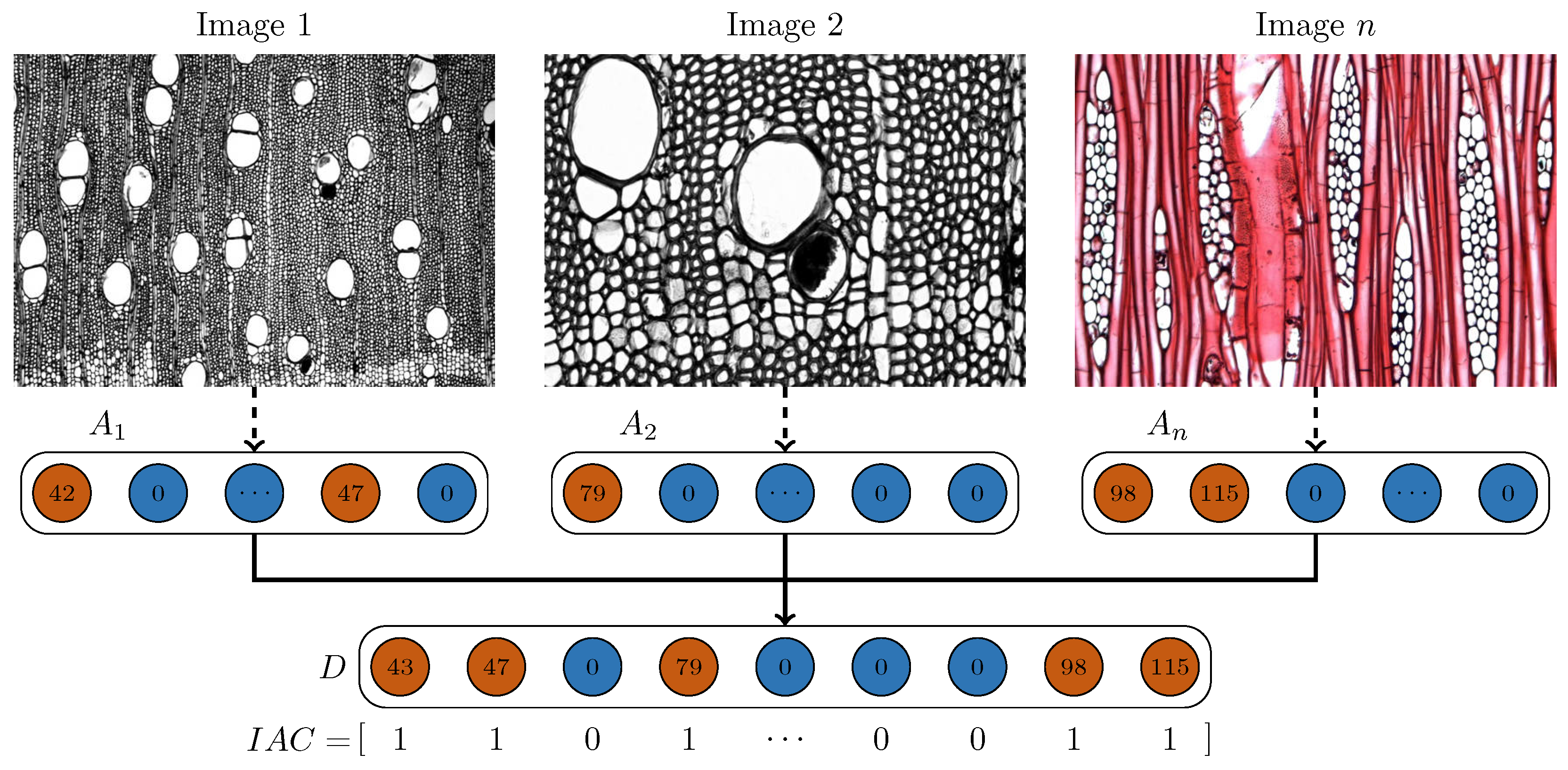
Figure 6.
Multi-image IAWA feature fusion process. Image 1 (specimen Kw 4353) yields IAWA feature codes 42 and 47; Image 2 (specimen Kw 4353) yields code 79; Image n (specimen Kw Swi.mac) yields codes 98 and 115. The codes are fused into a combined feature code set D, which is then binarized to generate the final feature vector IAC.
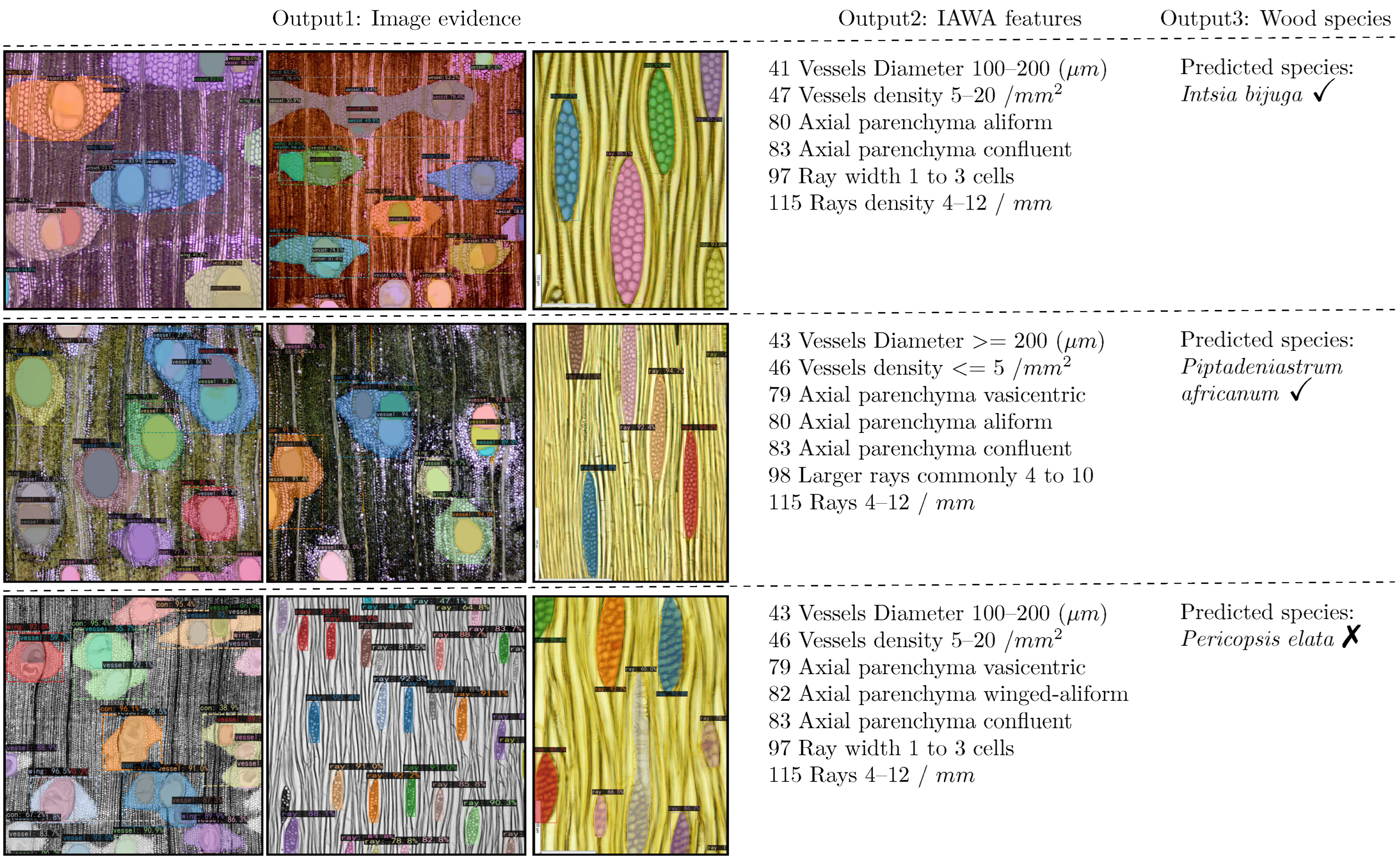
Figure 7.
Interpretable recognition results: Output1 provides image evidence, Output2 corresponds to the IAWA feature codes. Output3 represents the wood classification result. The first (specimen Tw 52896) and the second (specimens Tw 5225, Tw 6987) predictions are correct; the last one (specimens Tw 609, Tw 724) is incorrect—the correct species is Albizia ferruginea.
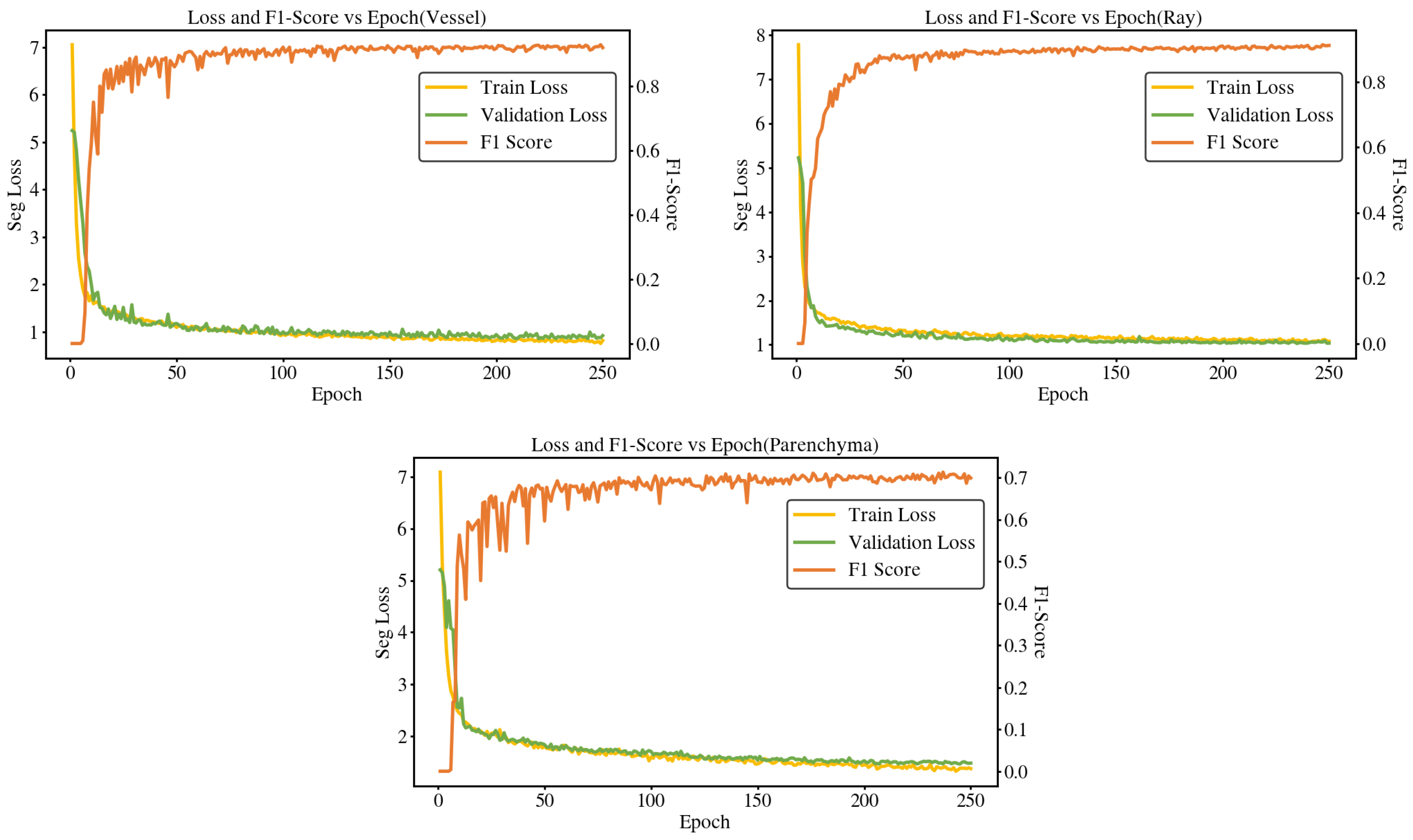
Figure 8.
Training loss and F1-score across epochs for different anatomical structures. The three plots correspond to vessel, ray, and parenchyma, respectively, showing training loss (left axis) and F1-score (right axis) over epochs.
Figure 8.
Training loss and F1-score across epochs for different anatomical structures. The three plots correspond to vessel, ray, and parenchyma, respectively, showing training loss (left axis) and F1-score (right axis) over epochs.
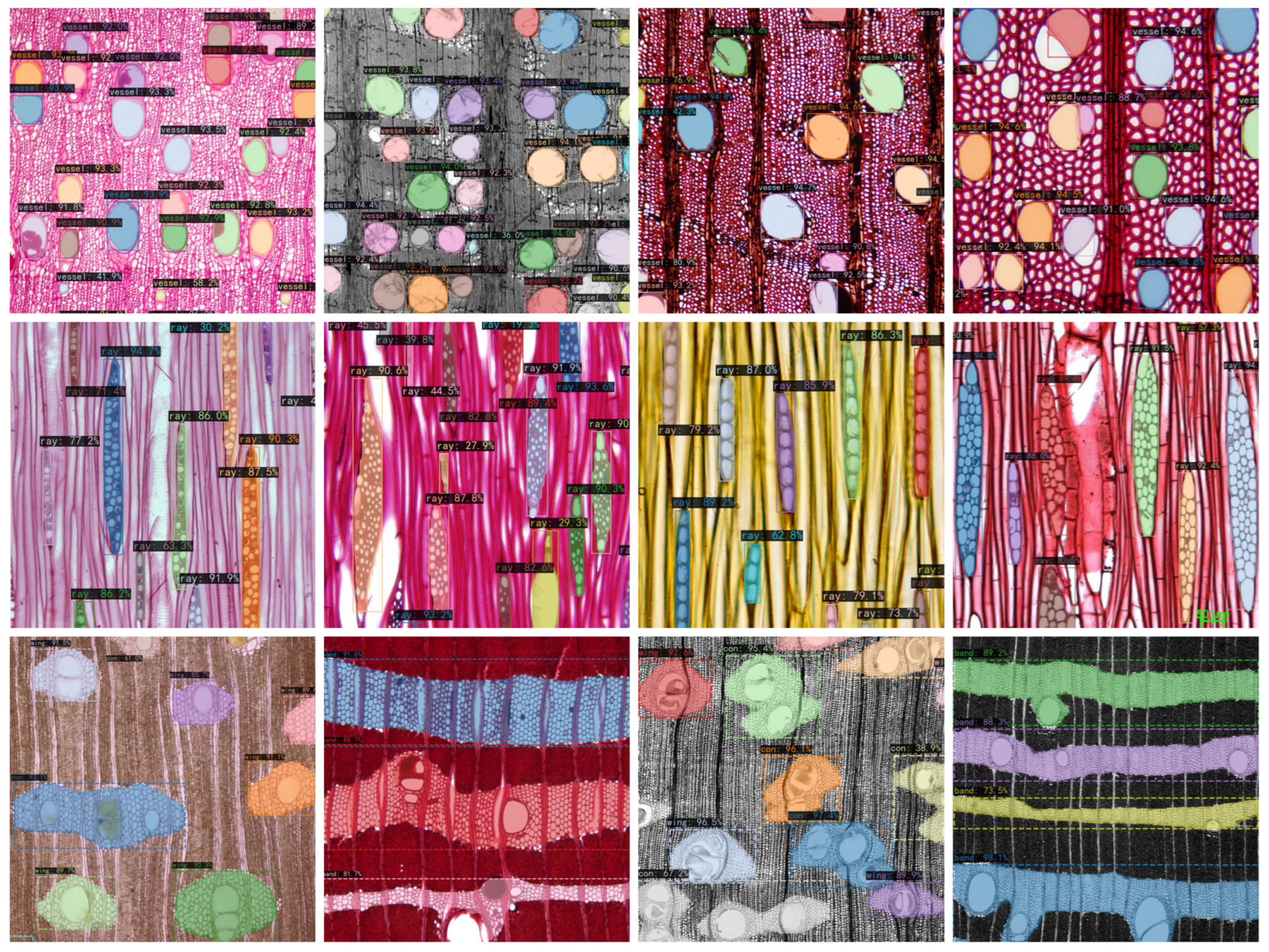
Figure 9.
Anatomy structure detection results. The first row (specimens Hw 23557, BWCw 8058, PACw 4673, and USw PR19) represents the vessel detection result, the second row (specimens BWCw 8332, USw PR19, Tw 5016, and Kw Swi.mac) represents the wood rays detection result, and the third row (specimens Tw 26885, Tw 609, and Tw 425) represents the parenchyma detection result.
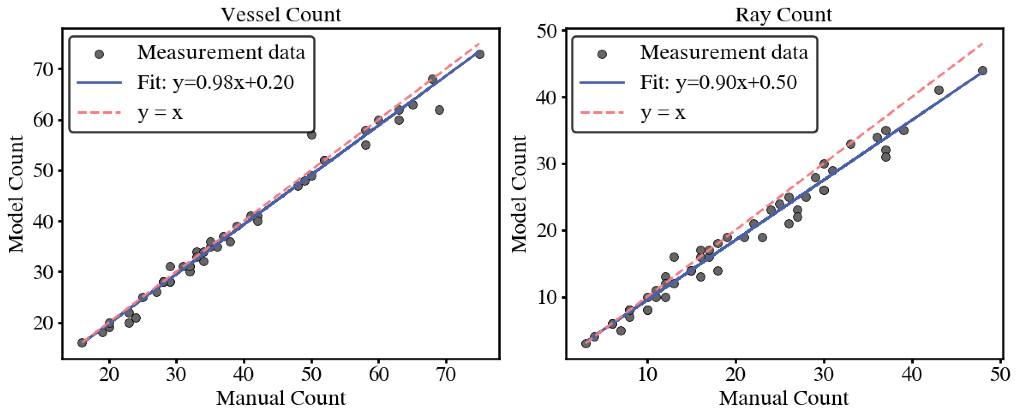
Figure 10.
Counting errors of vessels and wood rays between the proposed method and manual method.
Figure 10.
Counting errors of vessels and wood rays between the proposed method and manual method.
Figure 11.
Detection results of different models: The first column displays the original images, while the subsequent columns show the model-predicted images. The colors represent different anatomical structures. The first row (specimen FHOw 19992) correspond to vessel images, the second row (specimen FHOw 4291) is wood ray images, and the last row (specimen Tw 17698) represent parenchyma images.
Figure 12.
Impact of combining cross section and tangential section images on classification performance.
Figure 12.
Impact of combining cross section and tangential section images on classification performance.
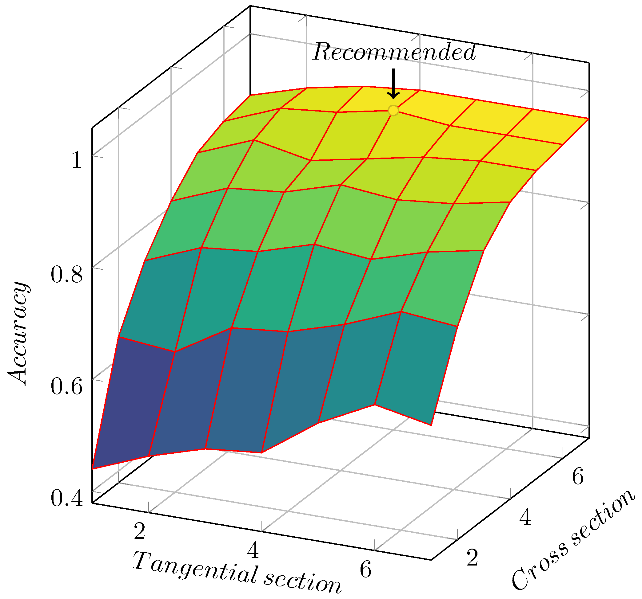
Figure 13.
Accuracy of image combinations with different quantities. The accuracy reaches its highest when there are 6 cross section images and 4 tangential section images.
Figure 13.
Accuracy of image combinations with different quantities. The accuracy reaches its highest when there are 6 cross section images and 4 tangential section images.
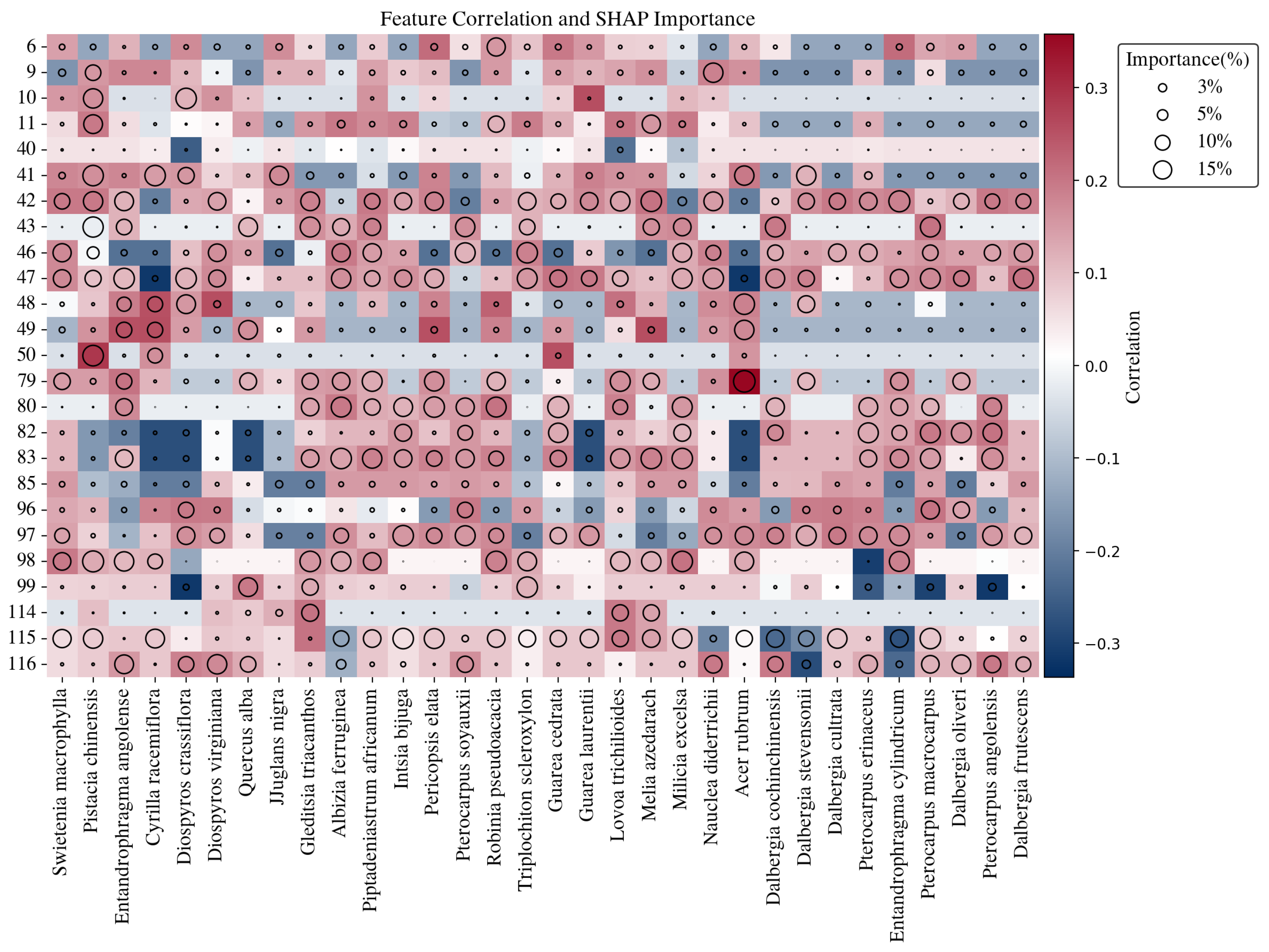
Figure 14.
Visualization of feature correlation and SHAP importance for IAWA features (y-axis) across wood species (x-axis). SHAP: a model-agnostic interpretability method based on cooperative game theory. It assigns each feature an importance value by quantifying its marginal contribution to the prediction across all possible feature combinations. Higher SHAP values indicate features that play a more decisive role in distinguishing between classes.
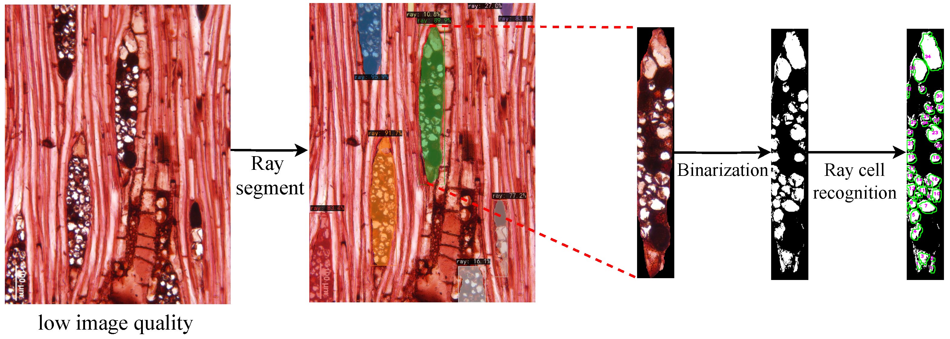
Figure 15.
Ray cell recognition under low image quality. The image (specimen PACw 4673) shows ray cells recognition results after segmentation and binarization under low image quality conditions.
Figure 15.
Ray cell recognition under low image quality. The image (specimen PACw 4673) shows ray cells recognition results after segmentation and binarization under low image quality conditions.
Table 2.
Wood species information in the dataset. The information includes Family, Species, WOCI (IAWA code 192: Wood of Commercial Importance) status, CITES listing, and Geographic Origin.
Table 2.
Wood species information in the dataset. The information includes Family, Species, WOCI (IAWA code 192: Wood of Commercial Importance) status, CITES listing, and Geographic Origin.
| ID | Family | Species | WOCI | CITES Listed | Geographic Origin |
|---|
| 1 | MELIACEAE | Swietenia macrophylla | ✓ | ✓ | (183, 184) |
| 2 | ANACARDIACEAE | Pistacia chinensis | | | (164, 167, 171, 173) |
| 3 | MELIACEAE | Entandrophragma angolense | ✓ | | (178, 179) |
| 4 | EBENACEAE | Cyrilla racemiflora | | | (182) |
| 5 | EBENACEAE | Diospyros crassiflora | ✓ | ✓ | (178, 179) |
| 6 | EBENACEAE | Diospyros virginiana | ✓ | | (184) |
| 7 | FAGACEAE | Quercus alba | ✓ | | (184) |
| 8 | JUGLANDACEAE | Juglans nigra | ✓ | | (182) |
| 9 | LEGUMINOSAE CAESALPINIOIDEAE | Gleditsia triacanthos | ✓ | | (182) |
| 10 | LEGUMINOSAE CAESALPINIOIDEAE | Albizia ferruginea | ✓ | | (178, 179) |
| 11 | LEGUMINOSAE CAESALPINIOIDEAE | Piptadeniastrum africanum | ✓ | | (178, 179) |
| 12 | LEGUMINOSAE DETARIOIDEAE | Intsia bijuga | ✓ | | (168, 169) |
| 13 | LEGUMINOSAE PAPILIONOIDEAE | Pericopsis elata | | ✓ | (178, 179) |
| 14 | LEGUMINOSAE PAPILIONOIDEAE | Pterocarpus soyauxii | ✓ | ✓ | (178, 179) |
| 15 | LEGUMINOSAE PAPILIONOIDEAE | Robinia pseudoacacia | ✓ | | (182) |
| 16 | MALVACEAE HELICTEROIDEAE | Triplochiton scleroxylon | ✓ | | (178, 179) |
| 17 | MELIACEAE | Guarea cedrata | ✓ | | (178, 179) |
| 18 | MELIACEAE | Guarea laurentii | ✓ | | (178, 179) |
| 19 | MELIACEAE | Lovoa trichilioides | ✓ | | (178, 179) |
| 20 | MELIACEAE | Melia azedarach | ✓ | | (164, 166) |
| 21 | MORACEAE | Milicia excelsa | ✓ | | (178, 179) |
| 22 | RUBIACEAE | Nauclea diderrichii | ✓ | | (178, 179) |
| 23 | SAPINDACEAE | Acer rubrum | | | (182) |
| 24 | FABACEAE | Dalbergia cochinchinensis | ✓ | ✓ | (171, 172) |
| 25 | FABACEAE | Dalbergia stevensonii | | ✓ | (184) |
| 26 | FABACEAE | Dalbergia cultrata | ✓ | ✓ | (171, 172) |
| 27 | FABACEAE | Pterocarpus erinaceus | ✓ | ✓ | (178, 179) |
| 28 | MELIACEAE | Entandrophragma cylindricum | ✓ | | (178, 179) |
| 29 | FABACEAE | Pterocarpus macrocarpus | ✓ | | (171, 172) |
| 30 | FABACEAE | Dalbergia oliveri | | ✓ | (171, 172) |
| 31 | FABACEAE | Pterocarpus angolensis | ✓ | ✓ | (178, 179) |
| 32 | FABACEAE | Dalbergia frutescens | ✓ | ✓ | (183) |
Table 3.
Selected IAWA feature codes and the descriptions.
Table 3.
Selected IAWA feature codes and the descriptions.
| IAWA Code | Description |
|---|
| Vessel arrangement and groupings |
| 6 | Vessels in longitudinal bands |
| 9 | Vessels exclusively solitary (90% or more) |
| 10 | Vessels in radial multiples of 4 or more common |
| 11 | Vessel clusters common |
| Tangential diameter of vessel lumina |
| 40 | <=50 μm |
| 41 | 50–100 μm |
| 42 | 100–200 μm |
| 43 | >=200 μm |
| Vessels per square millimetre |
| 46 | <=5 vessels per square millimetre |
| 47 | 5–20 vessels per square millimetre |
| 48 | 20–40 vessels per square millimetre |
| 49 | 40–100 vessels per square millimetre |
| 50 | >=100 vessels per square millimetre |
| Paratracheal axial parenchyma |
| 79 | Axial parenchyma vasicentric |
| 80 | Axial parenchyma aliform |
| 82 | Axial parenchyma winged-aliform |
| 83 | Axial parenchyma confluent |
| 85 | Axial parenchyma bands more than three cells wide |
| Ray width |
| 96 | Rays exclusively uniseriate |
| 97 | Ray width 1 to 3 cells |
| 98 | Larger rays commonly 4- to 10 seriate |
| 99 | Larger rays commonly > 10-seriate |
| Rays per millimetre |
| 114 | <=4/mm |
| 115 | 4–12/mm |
| 116 | >=12/mm |
Table 4.
Wood species classification results. The table presents the precision, recall, and F1-score for each species, along with the overall accuracy and weighted average metrics across all species. The weighted average accounts for the number of samples per species, giving more influence to species with more samples.
| Species | Precision | Recall | F1-Score |
|---|
| Swietenia macrophylla | 0.960 | 1.000 | 0.980 |
| Pistacia chinensis | 0.935 | 1.000 | 0.967 |
| Entandrophragma angolense | 1.000 | 0.962 | 0.980 |
| Cyrilla racemiflora | 0.895 | 1.000 | 0.944 |
| Diospyros crassiflora | 0.980 | 0.970 | 0.980 |
| Diospyros virginiana | 0.975 | 0.985 | 0.980 |
| Quercus alba | 0.944 | 1.000 | 0.971 |
| Juglans nigra | 0.980 | 0.990 | 0.985 |
| Gleditsia triacanthos | 0.909 | 0.833 | 0.870 |
| Albizia ferruginea | 0.692 | 0.818 | 0.750 |
| Piptadeniastrum africanum | 0.957 | 0.917 | 0.936 |
| Intsia bijuga | 0.867 | 0.929 | 0.897 |
| Pericopsis elata | 0.688 | 0.647 | 0.667 |
| Pterocarpus soyauxii | 1.000 | 0.950 | 0.974 |
| Robinia pseudoacacia | 0.885 | 1.000 | 0.939 |
| Triplochiton scleroxylon | 0.905 | 1.000 | 0.950 |
| Guarea cedrata | 0.941 | 0.889 | 0.914 |
| Guarea laurentii | 0.970 | 0.980 | 0.975 |
| Lovoa trichilioides | 0.895 | 0.773 | 0.829 |
| Melia azedarach | 0.737 | 0.778 | 0.757 |
| Milicia excelsa | 0.824 | 1.000 | 0.903 |
| Nauclea diderrichii | 0.938 | 0.833 | 0.882 |
| Acer rubrum | 1.000 | 0.900 | 0.947 |
| Dalbergia cochinchinensis | 1.000 | 0.950 | 0.974 |
| Dalbergia stevensonii | 0.933 | 1.000 | 0.966 |
| Dalbergia cultrata | 0.960 | 1.000 | 0.980 |
| Pterocarpus erinaceus | 1.000 | 0.857 | 0.923 |
| Entandrophragma cylindricum | 0.965 | 0.975 | 0.970 |
| Pterocarpus macrocarpus | 1.000 | 0.913 | 0.955 |
| Dalbergia oliveri | 0.970 | 0.985 | 0.977 |
| Pterocarpus angolensis | 0.975 | 0.980 | 0.978 |
| Dalbergia frutescens | 0.960 | 0.970 | 0.965 |
| Accuracy | | | 0.941 |
| Weighted Average | 0.926 | 0.933 | 0.927 |
Table 5.
Hyperparameter settings used for YOLO-seg model training.
Table 5.
Hyperparameter settings used for YOLO-seg model training.
| Hyperparameter | Value | Description |
|---|
| epochs | 250 | Number of training epochs |
| batch | 16 | Batch size per iteration |
| imgsz | 640 | Input image size |
| learning_rate | 0.01 | Initial learning rate |
| optimizer | SGD | Type of optimizer |
| weight_decay | 0.0005 | Weight decay for regularization |
| momentum | 0.937 | Momentum factor for SGD |
Table 6.
Detection performance comparison of different models for anatomical structures. Metrics reported include Average Precision (AP) at IoU thresholds 0.50 (AP50) and 0.75 (AP75), and the mean Average Precision (mAP) across different IoU thresholds evaluated for vessel, ray, and parenchyma.
Table 6.
Detection performance comparison of different models for anatomical structures. Metrics reported include Average Precision (AP) at IoU thresholds 0.50 (AP50) and 0.75 (AP75), and the mean Average Precision (mAP) across different IoU thresholds evaluated for vessel, ray, and parenchyma.
| Model | Vessel | Ray | Parenchyma |
|---|
|
AP50
|
AP75
|
mAP
|
AP50
|
AP75
|
mAP
|
AP50
|
AP75
|
mAP
|
|---|
| Mask-RCNN | 0.770 | 0.747 | 0.646 | 0.948
| 0.811 | 0.674 | 0.760 | 0.582 | 0.494 |
| PointRend | 0.741 | 0.705 | 0.596 | 0.930 | 0.806 | 0.674 | 0.531 | 0.501 | 0.457 |
| CondInst | 0.764 | 0.660 | 0.544 | 0.903 | 0.613 | 0.551 | 0.533 | 0.496 | 0.471 |
| YOLOv8-seg | 0.912 | 0.864 | 0.715 | 0.935 | 0.834 | 0.716 | 0.730 | 0.623 | 0.572 |
Table 7.
Recognition accuracy of five classification models evaluated on the train set and test set.
Table 7.
Recognition accuracy of five classification models evaluated on the train set and test set.
| Model | Accuracy of Test Set | Accuracy of Train Set |
|---|
| SVM | 0.939 | 0.946 |
| Naive Bayes | 0.941
| 0.945 |
| Decision Tree | 0.900 | 0.973 |
| Random Forest | 0.937 | 0.942 |
| KNN | 0.921 | 0.940 |
