Article

Genetic Variation Associated with Leaf Phenology in Pedunculate Oak (Quercus robur L.) Implicates Pathogens, Herbivores, and Heat Stress as Selective Drivers

1
Center for Ecology and Evolution in Microbial Model Systems EEMiS, Department of Biology and Environmental Science, Linnaeus University, SE-391 82 Kalmar, Sweden
2
Department of Physics, Chemistry and Biology (IFM), Linköping University, SE-581 83 Linköping, Sweden
3
Department of Forestry and Wood Technology, Linnaeus University, SE-351 95 Växjö, Sweden
*
Authors to whom correspondence should be addressed.
These authors contributed equally, should be considered joint senior authors and have the right to place their name last in the CV.
Forests 2025, 16(8), 1233; https://doi.org/10.3390/f16081233 (registering DOI)
Submission received: 23 June 2025 / Revised: 15 July 2025 / Accepted: 22 July 2025 / Published: 26 July 2025
(This article belongs to the Special Issue Woody Plant Phenology in a Changing Climate, 2nd Edition)

Abstract

Leaf phenology of trees responds to temperature and photoperiod cues, mediated by underlying genes and plasticity. However, uncertainties remain regarding how smaller-scale phenological variation in cold-limited regions has been affected by modified selection pressures from herbivores, pathogens, and climate conditions, and whether this leaves genetic signatures allowing for projections of future responses. We investigated environmental correlates and genetic variation putatively associated with spring and autumn leaf phenology in northern range margin oak (Quercus robur L.) populations in Sweden (55.6° N–60.8° N). Results suggested that budburst occurred later at higher latitudes and in locations with colder spring (April) temperatures, whereas leaf senescence occurred earlier at higher latitudes. Several candidate loci associated with phenology were identified (n = 40 for budburst and 47 for leaf senescence), and significant associations between these loci and latitude were detected. Functions associated with some of the candidate loci, as identified in previous studies, included host defence and heat stress tolerance. The proportion of polymorphic candidate loci associated with budburst decreased with increasing latitude, towards the range margin. Overall, the Swedish oak population seems to comprise genetic diversity in phenology-related traits that may provide resilience to a rapidly changing climate.

1. Introduction

Leaves are the part of the tree that is responsible for photosynthesis and thereby a necessary component for the uptake of carbon and assimilation into growth. The period of the year when photosynthesis takes place, as indicated by visible changes to the leaves during the year, may be termed the ‘phenological growing season’ [1]. For deciduous trees, these changes include the emergence of leaves in spring and the loss of greenness and often leaf abscission in the autumn. Because this cycle is a response to seasonally varying conditions, it is generally annual in temperate deciduous species [1]. For deciduous trees that persist in temperate regions where they experience temperatures that are harmful to their leaves during large parts of the year, a key adaptation is the timing of the phenological growing season [2]. Further, the ability to regulate the start and end of this season has been cited as a determinant of the range limits of deciduous species ([3]; but see also [4], who argue against the direct role of temperature).
In a larger perspective, understanding how leaf phenology responds to temperature is relevant to understanding the potential short-term adaptive response of forests to climate change [5]. Earth systems models predict that the Swedish climate will become warmer, which is likely to be associated with phenological shifts, including advancements and postponements of spring phenology and autumn phenology, respectively [6]. This will likely result in longer growing seasons, with the direction and magnitude of these trends varying between species and according to location [7]. Climate change is expected to result in modified selection pressures and concomitant changes in the alleles that are beneficial in a given part of the species range [8]. Southern and mid Sweden are of particular interest, as these regions include the northern range margin of Quercus robur (L.), and because the variability and magnitude of temperature increase are expected to be higher at high-latitude regions [9]. Therefore, describing allelic variation in the loci putatively associated with leaf phenology may help identify potentially vulnerable parts of the population and inform future conservation efforts [10].

1.1. Background

The response of budburst timing to temperature and photoperiod may be complementary. Experimental evidence based on cuttings from Q. robur and the sessile oak (Quercus petraea (Matt.) Liebl.) suggests that a longer photoperiod accelerates budburst, and that the effect of photoperiod may be dampened by chilling [11,12]. This may indicate that sensitivity to photoperiod diminishes past a certain stage of bud development [12]. Additional factors that may affect the timing of budburst in trees include precipitation (Kuster et al. [13] (but see Morin et al. [14], who find no effect)), humidity [15], soil nutrients [16], and CO2 concentration [17]. However, these factors are only expected to explain a minor share of the total regional variation in budburst [13,18,19].
For leaf senescence, photoperiod has been identified as the primary source of latitudinal variation, with temperature being less important [20]. However, there is less research on the drivers of variation in leaf senescence compared with budburst, and these are more poorly understood [21]. Besides insolation, leaf senescence is influenced by soil moisture, precipitation, and temperature in the month preceding senescence [22], as well as the pathogen load [23]. Similar to budburst, the drivers of leaf senescence seem to vary between species [19]. Several authors also report a positive association between the timing of budburst and leaf senescence within populations on scales up to European-wide [24,25,26], but it should be noted that this pattern has been found to vary depending on the timing of spring warming, possibly due to an interaction with photoperiod [27].
The timing of budburst and leaf senescence onset has consequences for the growth of the tree [28]. Mistiming budburst in spring with respect to the occurrence of frost can be devastating due to the severe cost of shooting reserve buds [29]. Such mistiming will likely become more frequent in the impending climate because of advancing budburst, more variable spring temperatures [30], and increased risk of frost during the early stages of leaf emergence when the leaves are less freeze-tolerant [31]. Biotic stressors such as herbivory and fungal infection have also been identified as sources of leaf damage with negative implications for tree growth [32], as well as fecundity [33]. The extent of defoliation and fungal infection endured may also depend on the phenological synchrony between the tree and the biotic stressors, something that is predicted to change due to differing phenological responses to future temperature changes [34]. In autumn, mistiming leaf senescence may also induce frost damage and a lost opportunity to reabsorb nutrients [20]. However, the body of the literature investigating frost damage in spring is much larger than that which is concerned with autumn mismatch, possibly because the consequences of frost damage for the tree are assumed to be more severe in spring [35].
Multiple studies in which seeds of varying provenance have been reared in common gardens report significant heritability in budburst in Q. robur and Q. petraea [36,37]. Heritability is the potential for future responses of a trait to selection, as well as that of genetically correlated traits [38], and it has been suggested that defences to biotic stressors have a genetic basis [39,40]. Additionally, it has been found that variation in the relative timing of budburst and leaf senescence among individuals within stands is largely consistent between years [24,25], which may reflect genetic differences [25]. It has further been suggested that among the adaptive responses to herbivory and fungal infection are shifts in leaf phenology that induce mismatch [41].
Evidence is also accumulating that a sizable share of the regional variation in leaf phenology has an underlying genetic basis. Using targeted sequencing of genes associated with leaf phenology by differential gene expression [42,43,44], it has been possible to test for associations of these genes with spatial patterns and environmental drivers [45]. After finding associations between a subset of these genes and timing among the sampled individuals, Alberto et al. [45] also report significant associations with latitude and temperature, interpreted as signatures of adaptation in genes associated with leaf phenology. The distribution of Q. robur in Sweden spans a substantial latitudinal gradient in seasonality and the length of the growing season, and the range edge occurs in the transition between the boreo-nemoral and the boreal zones (dominated by conifers) [46]. Therefore, the Swedish Q. robur population represents an important part of the species range for investigating adaptations in leaf phenology.

1.2. Aims and Hypotheses

The overarching aim of this study was to increase the understanding of the drivers of genetic variation associated with leaf phenology by identifying genetic signatures associated with phenological traits and investigating geographic patterns across the species’ distribution range in Sweden. The aim was broken down into the following sub-aims: (i) temperature and latitude are cues of leaf phenology, and leaf senescence has been found to covary with budburst, so these were investigated for the Swedish range; (ii) functions related to leaf phenology and its drivers were identified among the loci associated with relative leaf phenology; and (iii) signatures of selection were explored among the candidate loci, as spatial heterogeneity in temperature and other suggested drivers exists in the Swedish range.

2. Materials and Methods

2.1. Study Species, Sampling Locations, and Data Collection

Quercus robur is a monoecious tree that disperses its pollen by wind and seeds by animals and gravity [47]. Previous studies suggest that they are predominantly outcrossing, and the share of paternity from trees within the stand may depend on the topography [48,49]. The species is found throughout most of Europe, its distribution extending from the Iberian Peninsula, Italy, and the northern Balkans in the south to the United Kingdom, southern to mid Sweden, and the Baltic in the north [50].
The study was conducted in oak forest stands situated in the south central region of Sweden, an area covering 130,000 km2 and comprising various ecological zones and a mosaic dominated by forests, farmland and lakes, and spanning >5 degrees latitude (55.6° N–60.8° N) extending up to Gävle, the current northern range margin for naturally occurring Q. robur in Sweden (Figure 1). Southern Sweden is in the temperate climate zone, characterised by relatively warm summers and mild winters. Temperatures can drop well below freezing, and snowfall is not uncommon, but the length and severity of winter differ between regions, with longer and colder winters naturally occurring in the north. During the past 120 years, the climate in Sweden has moved northward at an alarming rate, with the temperature increase being most pronounced in the northern regions (see Figure 2 in Sunde et al. [51]). As a result of climate change, maximum air temperatures in the study area are projected to increase well above current temperatures within the next 50 years (see Figure 2 in Forsman et al. [52]).
The study integrates three types of data: on the tree level, estimates of phenological progress made during the spring and autumn of 2023 and reference aligned restriction-site associated DNA sequencing (RADseq) data, and on the stand level hourly temperature data (used to assess the accuracy of interpolated data obtained from the Swedish Meteorological and Hydrological institute (SMHI) (see Section 2.1.2) with varying coverage. The sampling of spring and autumn phenological progress (see Section 2.1.1.) was carried out for 10 oak trees in each of 10 stands, distributed along a latitudinal gradient in southern Sweden (Figure 1). The mean distance between trees within stands was 65 m (SD = 36 m). The sampled trees were healthy and dominant (when considering crown development and height relative to neighboring trees). Due to sequencing failures (n = 4) and the identification of trees as being either Q. petraea or Q. robur × Q. petraea hybrids based on genetic clustering and leaf morphology (n = 15) [53], all stands did not contribute data for all 10 sampled individuals as we only included trees assigned “pure” Q. robur in the subsequent analyses. The final data set comprised 81 Q. robur from 9 stands, with the number of individuals per stand varying between 6 and 10 (Figure 1). One stand (Bellinga) was a plantation consisting of trees planted in 1995, with acorns from various locations in southern Sweden [54]. Information on the size of study areas, landscape context, soil type, species composition of bushes and trees, and age of sampled oaks is available elsewhere (see Table S1 in Johansson et al. [55]).

2.1.1. Leaf Phenology Scoring Method

To quantify the phenological progress (leaf development) of the oaks in the spring, weekly (mean ± SD: 7.3 ± 0.8 days) observations were performed between 23 April and 5 June 2023, with the leaf development stage being determined using binoculars. To this end, each tree was observed on three to five occasions, depending on when the leaves reached full emergence. For each tree and on each occasion, leaf development stage was scored from the four cardinal directions. The scoring classification system used largely follows Faticov et al. [56]. Briefly, we used a categorical system where 1 represents small and dormant buds, 2 larger buds with a hint of green, 3 elongated buds with leaves starting to emerge (i.e., bud burst), 4 leaves emerging but still close together, 5 leaves separated but not yet fully expanded, and 6 leaves fully expanded and with a darker green colour (see Figure 1B).
To measure the onset of leaf senescence in the autumn, each tree was observed four to six times (mean interval of 14.1 ± 2.3 days) between 11 September and 27 November. On each sampling occasion, the proportion of green, yellow, and brown foliage was scored for each tree. For the following analyses, we used the proportion of green leaves as a proxy for the processes associated with the end of the photosynthetic period, from here on referred to as leaf senescence [57]. There were five instances among four trees where observations made later than the previous observation showed lower phenological progress. These observations were excluded from the dataset. All scoring was performed by the same person (J. Lundqvist).
We then used the observations to fit a sigmoidal curve from which the date of budburst was estimated for each tree. Leaf senescence onset dates were obtained in a similar way, by fitting a curve based on weekly observations (from 11 September to 27 November 2023) on the progress of leaf colouration (percentage of green leaves remaining on the tree). This method is described in greater detail in Appendix A.1.

2.1.2. Temperature Data

Temperature data were collected to investigate associations with phenology and genetic diversity. To this end, variables representing spring and autumn temperatures in 2023 at each stand were calculated as daily means of temperatures in April and August, respectively. The months of April and August were chosen because these months represented temperatures before most budburst or leaf senescence onset dates, respectively, occurred. To obtain temperature estimates for each stand, publicly available interpolated grid data with a resolution of 4 km from SMHI were used (available at: https://www.smhi.se/data/ladda-ner-data/griddade-nederbord-och-temperaturdata-pthbv, accessed on 10 July 2025; the interpolation method is described in Johansson [58]). The accuracy of these data was assessed by comparing them with temperature data collected in situ, as well as from additional stands using HOBO loggers (Onset Computer Co., Bourne, MA, USA) (Appendix A.2). The assessment strategy was to compare data specific to the periods where temperature data were used. Overall, the accuracy was high (mean absolute errors for April and August: 0.41 and 1.18; R2 values: 0.93 and 0.91). The decision against using data collected with temperature loggers was justified by the fact that temporal coverage varied between stands, which would have implied a severe loss of data (each stand representing ~11% of the total observations). Long-term monthly minimum temperature means for April and August from 1961–2023 were also obtained for each stand using the SMHI dataset. These data were used to evaluate associations between local climatic temperatures and temperature requirements (see Section 2.2), as well as genetic diversity indices.

2.2. Statistical Testing for Associations of Temperature and Latitude with Phenology

To test if temperature and latitude were associated with phenology, individual timings for each tree were used as dependent variables in linear mixed models with temperature variables and latitude as fixed effects with a random intercept for repeated measures on the “stand” group. Covariance between budburst and leaf senescence was tested by also including budburst date as a fixed effect in the models predicting leaf senescence. Linear mixed models were fitted using the glmmTMB function in the package glmmTMB (v1.1.9; [59]). To determine if significant associations may have been due to effects on the variance of the dependent variable, dispersion was modelled against the significant variables as well. All associations were tested for significance using a Type 2 Wald test in the Anova function in the car package (v3.1-2; [60]). Additionally, the variation explained in the model with and without random components was calculated as the marginal R2 (R2M) from the conditional R2 (R2C), as implemented in the r.squaredGLMM function in the MuMIn package (v1.48.11; [61]).
Variation in heating requirements was also investigated, but these results proved inconclusive and did not add qualitatively to the analysis. However, they are included in the Supplementary Materials (Supplement S1).

2.3. Acquisition of RADseq Data

2.3.1. DNA Extraction and Sequencing

Leaves from 10 trees per stand for which leaf phenology was observed in 2023 were collected and stored in −20 °C. About 70 mg of plant material was homogenised with stainless steel beads (Next Advance, Troy, NY, USA). After homogenisation, DNA was extracted using the DNeasy Plant Pro kits (Qiagen, Valencia, CA, USA) following a slightly modified version (longer homogenization time for tough leaves) of the protocol provided by the manufacturer. DNA quality and quantity checks were done using a Qubit 2.0 fluorometer (absorption value ratio 260/320 nm) and a NanoDrop 2000 spectrophotometer (absorption value ratios 260/280 and 260/320 nm) (Thermo Fisher Scientific, Waltham, MA, USA). Samples were digested with HF EcoRI enzyme (New England Biolabs, Ipswich, MA, USA) for two hours at 37 °C, followed by 15 min of enzyme inactivation at 65 °C. Following digestion, Qubit was again used to quantify the amount of DNA, and gel electrophoresis was used to confirm successful digestion. Library preparation and sequencing were done by SciLifeLab (Uppsala, Sweden) on an S4 lane using the Illumina NovaSeq6000 (Paired-end, 2 × 150 bp setup). Sequences were demultiplexed before delivery.

2.3.2. Bioinformatics

The Stacks pipeline [62] was used to obtain the SNP genotype matrix used in the genotype–phenotype association. The first step of the pipeline was process_radtags, which corrected restriction sites and then removed reads unless they met the following criteria: (i) there were no uncalled bases; (ii) when running a sliding window of the size 15% of the read length along it, the bases in each length needed to have an average probability of a correctly called base of 99%. Further quality checks were done using FastQC (v0.11.9; [63]) and MultiQC [64]. In the next step, the sequences were mapped to a reference genome (NCBI accession: GCF_932294415.1) using the Burrows-Wheeler Alignment tool [65]. SAMtools (v1.20; [66]) was used with default settings to convert the output to the binary alignment map format (.bam) and sort the reads by coordinates.
These sorted reads were subsequently used as input in the gstacks module to produce a catalogue of SNP genotypes for each individual. Then, the populations module was run, filtering out loci which did not meet the following criteria: (i) the locus had to occur in 80% of individuals within each stand; (ii) the locus had to have a minor allele frequency of 5% across all individuals; (iii) the observed heterozygosity was not allowed to exceed 70%. These requirements were set to ensure that loci were well replicated throughout the stands and to avoid including alleles that were genotyping errors [67]. In this filtration step, 876,331 loci were filtered out from an initial 928,319. To reduce biases associated with linkage, it was further specified that one randomly selected SNP be chosen to represent the locus. The number of variant sites resulting from this was 17,934. The output was specified to be in pedigree format (.ped) with an accompanying variant information file (.map) for input in Plink (v1.90b4.9; [68]). This was necessary because duplicate loci (which were identified after examining the file in variant calling format (.vcf) of the output) existed that needed to be excluded before imputation. This was also done in Plink using the --exclude flag, leaving 16,903 loci. Finally, imputation of missing loci was done using the genotype imputation algorithm implemented in Beagle (v5.4; [69]) with default settings.

2.4. Analysis of Genetic Variation Associated with Phenology

To identify loci that were statistically associated with relative budburst or leaf senescence, the timing of each individual was first standardised with respect to timings within each stand to obtain stand-relative timings. Thus, the earliest individual within each stand would have the same value, and each stand has the same mean and variance. This was done to account for variation in timings due to the effects of local temperatures on temperature requirements that may arise during each individual’s lifetime (see [18,70]). However, there was a lack of variance in budburst in two of the stands, Testeboån and Vårgårda, so a subset was created, excluding these stands from the genotype–phenotype association analysis for relative budburst (n = 64).

2.4.1. Investigating Population Structure

When performing genotype–phenotype associations, it is not uncommon that population structure leads to spurious associations, because divergence is also in the neutral parts of the genome [71]. Therefore, it is common practice to statistically control for population structure. By standardising means and variances of the budburst and leaf senescence dates within stands, associations due to stand-level variation are mitigated, and the study design, as such, partly controls for population structure. However, if population structuring is weak and gene flow is ample, with paternity often coming from trees outside the stand [47], structure could overlap across stands and might have manifested on spatial scales that differed from the groupings of the sampling locations. Furthermore, one of the included stands, Bellinga, contains trees of allochthonous provenance. Additionally, in stands where the distribution of timings was heavily skewed and the underlying variation likely poorly represented (Lin et al. [72], for example, report normally distributed timings), it was feared that while the few individuals with timings that differed from the majority of other individuals in the stand may have had different alleles in the loci that were truly associated with timing, they may also have had different alleles at putatively neutral loci, due to population structuring. Therefore, correlations between population structure and relative timings were investigated to evaluate whether population structuring seemed to drive potential patterns and needed to be accounted for further. For this, Pearson’s correlation coefficients between eigenvectors obtained in a principal coordinates analysis (PCoA) of Manhattan distances between individuals and their relative timings were calculated. The number of ordination axes to consider was determined using a broken stick criterion ([73] cited in [74]) and Cattell’s rule [75]. The broken stick criterion compares the variance explained by each principal component to the variance explained if the total variance were randomly distributed among them, where those components that explain less variance than that obtained from the random data are deemed uninteresting ([73], cited in [74]). Cattell’s rule instead states that only principal components to the left of the “elbow” where the variance explained by each axis starts to plateau out should be considered for interpretation [75]. Lastly, the number of ancestral populations was estimated using fastStructure (v1.0, [76]) (after producing a valid input file in browser extensible format (.bed) in Plink) to determine how many components in the genetic data to control for in the association methods.

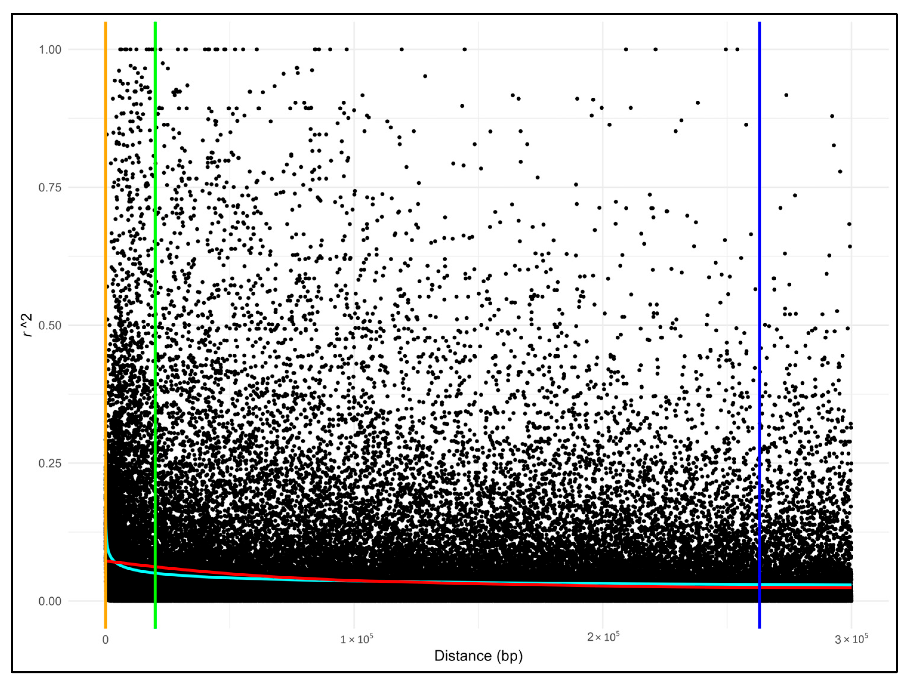
2.4.2. Linkage Decay

Because of linkage, the specific positions of the outlier SNPs identified do not necessarily have to be located within the genomic region coding for a trait; they may be inherited together with coding loci due to their proximity on the chromosome ([77], pp. 44–45). When comparing with regions associated with a certain function in the annotated genome, it is therefore useful to consider if the locus exists within a certain number of basepairs either side of the candidate locus instead of only checking if the candidate locus falls within the region. To estimate the distance from the candidate locus to look in, squared correlation coefficients (r2) between loci of various distances up to 300 kbp were calculated using the programme PopLDdecay (v3.42; [78]). The linkage disequilibrium decay pattern was then estimated by fitting a LOESS regression and a power curve, with mean r2 as response variable and distance as independent variable. Different cut-offs for the number of basepairs from the candidate locus to look in when comparing candidate loci against the annotated genome are given in the literature. Some rely on an arbitrary low value (e.g., Otyama et al. [79] use 0.2), while others go by the distance at which the r2 value falls below half (e.g., Pang et al. [80]). In this dataset, the linkage disequilibrium decay fell below half at 263,035 bp using LOESS regression and 24 bp using a power curve (Appendix A.3). As neither seemed reasonable, the candidate loci were compared with the annotated genome within an arbitrary search distance of 20 kbp on either side of the locus (as a more conservative alternative to that obtained with the LOESS regression), while reporting the distance together with the genes identified in the results for transparency.

2.4.3. Genotype–Phenotype Association

Distance-based redundancy analysis (dbRDA) was used to identify candidate loci. It is a constrained ordination that allows the user to directly compare structures in a response matrix with explanatory variables ([81], p. 630). This multivariate approach considers multiple loci at once, allowing for the association of loci with a phenotype where genic variance is low, but the covariance of allelic effects is high [82,83]. Small allelic effect sizes have been observed for several tree species, and analytical evidence for the build-up of adaptive differentiation through covariance has been given as an explanation for the great phenotypic variation in other oak populations [45,84]. Two dbRDAs were carried out with a Manhattan distance matrix calculated from the full SNP genotype matrix as the dependent variable and the relative phenologies as explanatory variables (one analysis for budburst and one for leaf senescence). To test if the constrained axes represented structured and not random variation, permutation tests were carried out with 9999 permutations. The adjusted R2 (R2a) was also calculated for these axes. The dbRDAs and permutation tests were performed using the capscale and anova.cca functions, respectively, in the R package vegan (v2.6-4; [85]).
The loadings of loci obtained in the dbRDAs were converted to z-scores, which were used to calculate p-values [82]. To adjust for multiple hypothesis testing, q-values were calculated from the p-values using the R package qvalue (v2.34.0; [86]). The q-values were visualised in Manhattan plots produced using the R package ggplot2 (v3.5.1; [87]). The loci that had a q-value below 0.05 were included in the candidate loci and were compared with the annotated reference genome (from the same entry in NCBI as the genome used for alignment), as well as loci described by Bodénès et al. [88] who used a shotgun sequencing approach on chromosome 7, to determine if they could be found in regions previously associated with functions.

2.5. Regional Genetic Variation in Loci Putatively Associated with Leaf Phenology and the Neutral Dataset

To understand how genetic diversity among candidate loci identified in the genotype–phenotype association varied in the Swedish range, the following statistics were calculated for each stand: private alleles (PAs), the proportion of polymorphic loci (P), and the mean distance from the centroid in principal coordinate space. These were also calculated for the full dataset for comparison. To test if a significant share of the variation existed between stands, AMOVAs [89] were carried out for the sets of candidate loci identified as associated with budburst and leaf senescence, as well as the full dataset. Significance was determined using a permutation test with 9999 grouping permutations. AMOVAs were carried out using the amova function in the pegas package in R (v1.3; [90]). Additionally, pairwise FST were calculated between all stands to quantify the share of genetic diversity due to differences in allele frequency between stands [91] as well as to visualise genetic differentiation between different stand combinations according to latitude. To test if latitude was associated with genetic variation among candidate loci putatively associated with phenology, dbRDAs were carried out for the candidate loci in the same way as described for the genotype–phenotype associations (see Section 2.4.3) with latitude as an independent variable. The same permutation test was used with 9999 permutations to test for significance.

3. Results

3.1. Patterns and Associations of Budburst and Senescence

The dates of budburst and leaf senescence were estimated for individuals from each stand (Figure 1C,D). The total variance was lower for budburst dates (σ2 = 19.77) than for leaf senescence dates (σ2 = 150.44). Almost all budburst dates in Tånnö, Vårgårda, and Testeboån were shared within stands (shown as compressed boxplots in Figure 1B). Timings differed significantly between stands (budburst: F = 4.14, d.f. = 8, p < 0.0001; leaf senescence: F = 5.93, d.f. = 8, p < 0.0001). Mean April temperatures decreased significantly with latitude (Bellinga: 6.24 °C, Testeboån: 5.53 °C; r = −0.85, d.f. = 7, p = 0.003), while mean August temperatures did not (Bellinga: 16.28 °C, Testeboån: 15.52 °C; r = −0.40, d.f. = 7, p = 0.29). The date of budburst was positively associated with latitude (Bellinga mean = 127.42, Testeboån mean = 133.64; Testeboån: 5.53 °C; β = 1.30, χ2 = 3.90, d.f. = 1, p = 0.048) and negatively associated with mean April temperature (β = −2.89, χ2 = 7.55, d.f. = 1, p = 0.001) (Table 1). The onset of leaf senescence occurred earlier at northern latitudes (Bellinga mean = 292.33, Testeboån mean = 275.00; β = −3.42, χ2 = 10.73, d.f. = 1, p = 0.001) and tended to occur later in stands with warmer August temperatures (β = 10.38, χ2 = 3.60, d.f. = 1, p = 0.06) (Table 1). In contrast with previous findings, budburst and leaf senescence onset were not associated (β = 0.21, χ2 = 0.18, d.f. = 1, p = 0.67).

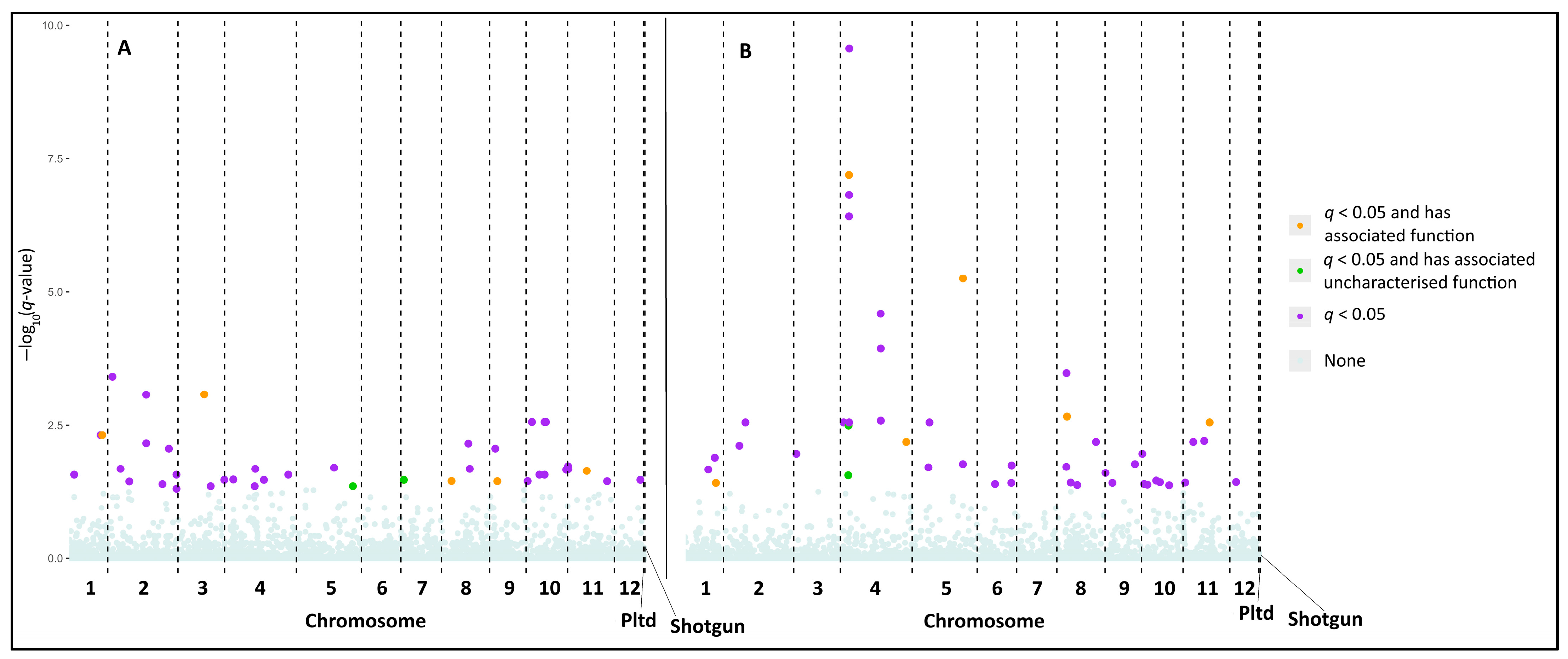
3.2. Loci Putatively Associated with Leaf Phenology

3.2.1. Population Structure

Using fastStructure, the most likely number of ancestral clusters was 1. When comparing the first 15 relative eigenvalues for the PCoAs with relative eigenvalues generated from a broken stick distribution, none of the first eigenvalues exceeded their broken stick counterparts (Appendix A.4). Additionally, the proportion of variance explained by each ordinal axis was low overall (axis 1 in the budburst and leaf senescence datasets represented 4.62% and 5.09% of the total variation, respectively, with proportionally small decreases for each subsequent axis) (Appendix A.4). Going by Cattell’s rule, a case could be made for the first three and four ordination axes to be considered for interpretation in the subset and the full dataset, respectively, as the decrease in relative eigenvalue diminished at those points. However, the covariances, estimated using Pearson’s correlation coefficients between the chosen eigenvectors and the standardised timings, were all low (|r| < 0.1, p > 0.5), indicating no significant association between the underlying population structure and relative phenology. Therefore, population structure was not partialled out of the dbRDAs before testing for associations with relative phenology.

3.2.2. Genotype–Phenotype Associations

In the dbRDAs, negative R2a values were obtained when calculating the share of genetic variance explained by the constrained axes (relative budburst: R2a = −0.002; relative leaf senescence: R2a = −0.001). This may indicate that relative budburst and relative leaf senescence explained a very small share of the genetic variance, that sample sizes were small, or a combination of the two, based on the equation used to calculate R2a ([81], p. 635). The hypothesis that the constrained axes represented structuring associated with timing was tested using permutation tests. That neither of these was significant (budburst: p = 0.92; leaf senescence: p = 0.79) indicates that neither relative budburst nor relative leaf senescence timings were important drivers of genetic structuring.
Associations between loci and standardised timings were estimated using dbRDAs, with q < 0.05 as a criterion for identifying candidate loci (Figure 2). The total number of candidate loci was 40 and 47 for relative budburst and relative leaf senescence, respectively. Associated loci were spread out across chromosomes.
Among the candidate loci, 5 and 6 of those associated with budburst and senescence, respectively, also had functions associated with them identified in previous studies not including those labelled as “Uncharacterised” (Table 2; a full list of candidate loci is found in Appendix A.5). Among the annotated genes associated with budburst that were characterised (Table 2), Transportin-1 is a nuclear import receptor binding to several specific proteins and RNA for transport from the cytoplasm to the nucleus [92]. In Arabidopsis thaliana (L.) Heynh., Yan et al. [93] find that Transportin-1 may be involved in the transport of several proteins, including those associated with defences against disease, stress tolerance, the circadian rhythm, flower development, and cold acclimation. Small nucleolar RNA R71 was also found, and is a small non-coding RNA that regulates gene expression [94] and has been associated with resistance to rust in pea (Pisum sativum L.) [95]. Another gene associated with defence, found among both the budburst and leaf senescence candidate loci, was identified as (−)-Germacrene D synthase-like, which has been associated with the heightened emission of an insecticidal terpene in response to herbivory in a hybrid poplar (Populus trichocarpa × deltoides Bartr.) [96]. A gene coding for the protein rRNA 2′-O-methyltransferase fibrillarin 1-like was also associated with budburst. Fibrillarin 1 is an enzyme that methylates ribosomal RNA, and has been found to increase in nuclear abundance in A. thaliana during recovery following a heat stress treatment [97]. Finally, MADS-box protein JOINTLESS-like was also found among the budburst candidate loci and is a protein similar to the MADS-box gene JOINTLESS, which has been found to affect the rate of growth in the shoot meristem of peppers (Capsicum spp.) [98] and the development of the abscission zone in tomato (Solanum lycopersicum L.) [99].
Among the 6 loci associated with leaf senescence found in the annotated genome (Table 2) was Mediator of RNA polymerase II transcription subunit 25, which has been found to affect flowering time via light perception in barley (Hordeum vulgare L.). Another gene was G-type lectin S-receptor-like serine/threonine-protein kinase At1G67520, a pattern recognition receptor that has been found to be associated with defence mechanisms against pathogens in Japanese chestnut [100] and in A. thaliana [101]. A second pattern recognition receptor among the leaf senescence loci associated with disease resistance was Putative disease resistance RPP13-like protein 1, which is upregulated in a line of Rose (Rosa L.) resistant to powdery mildew in response to inoculation [102]. A locus within the coding region responsible for Putative calcium-transporting ATPase 13, plasma membrane-type, which is involved in calcium transport [103], was also identified. It has been associated with several different functions in several different species: in the Huangguan pear (Pyrus bretschneideri Rehd.), it is associated with potassium availability, as potassium appears to also affect the uptake of calcium [104], in guman (Casuarina glauca Sieb. ex Spreng.) it is involved in the response of branchlets to salt stress [105], it is upregulated in tubers experiencing cold stress [103] and in the common grape vine (Vitis vinifera L.) it is positively modulated in response to pathogen inoculation [106]. Finally, a locus associated with leaf senescence was found in the coding region for Vacuolar-sorting receptor 3-like (Table 2), which detects internal and external changes to the cell, and has been found to be associated with the response to drought and heat stress in maize (Zea mays L.) [107].

3.3. Variation in the Full SNP Dataset and in Loci Putatively Associated with Phenology

3.3.1. Genetic Diversity Indices

To understand how genetic diversity varied and was partitioned across space, the number of private alleles (PAs), the proportion of polymorphic loci (P), and the mean distance from the centroid in principal coordinate space were calculated for each stand (Table 3). No PAs were found for the candidate loci, but in the full dataset, these ranged between 54 and 229. In the full dataset, P ranged between 0.53 and 0.69, which was lower than among the candidate loci: for the budburst loci, P ranged between 0.88 and 0.98, whereas for the leaf senescence loci, P ranged between 0.91 and 1.00. For genetic variability within sites, the mean Manhattan distance from the centroid in principal coordinate space ranged between 2890.13 and 3839.84 in the full dataset, between 16.89 and 21.35 for the budburst loci, and between 0.13 and 0.27 for the leaf senescence loci (Table 3).
The number of PAs increased with latitude (r = 0.77, d.f. = 7, p = 0.01) and decreased with mean minimum April temperatures (r = −0.83, d.f. = 7, p = 0.01) in the full dataset, with Testeboån having the greatest number by far of all stands. It should be noted that latitude and mean minimum April temperatures were strongly correlated (r = −0.96, d.f. = 7, p < 0.0001). Among the loci associated with budburst, the proportion of polymorphic loci decreased significantly with increasing latitude (r = −0.75, d.f. = 7, p = 0.02) and tended to increase with mean minimum April temperatures (r = 0.66, d.f. = 7, p = 0.054). Dispersion was almost significantly associated with latitude as well (r = −0.66, d.f. = 7, p = 0.052). No other significant associations were found between measures of diversity and latitude or temperature.

3.3.2. Population Structuring in the Putatively Adaptive Candidate Locus Datasets

Spatial variation was found among the candidate loci. Using permutation tests, significant between-stand variances were found in AMOVAs in all three datasets (p < 0.05). In all three datasets, the majority of variation was found within stands (full: 90.9%; budburst: 92.5%; senescence: 95.9%). Using dbRDA, it was additionally found that some of the between-stand variation could be explained by latitude in the full dataset (p = 0.0001; R2a = 0.03) and among the loci associated with budburst (p = 0.002; R2a = 0.02). In the full dataset, genetic differentiation from other stands (Figure 3) was generally higher for Testeboån and Vinala, the two northernmost stands. This pair also represented the stands that were most differentiated from each other out of all three datasets (FST = 0.127). Few discernible patterns were found among the candidate loci. Compared with the other stands, Testeboån tended to be more different from the rest of the stands among the candidate loci.

4. Discussion

Leaf phenology is one of the traits allowing deciduous trees to persist in the temperate parts of the world [2]. Associations of leaf phenology with regional heterogeneity in the timing of spring and autumn freezing, suggested to be the primary drivers [108], is thought to reflect a combination of microevolutionary genetic modifications and phenotypic plasticity [18]. To characterise leaf phenology of oaks in Sweden, identify environmental and genetic correlates of phenology, and enable future projections of how phenology may be affected by a changing climate, we integrated phenotypic, genetic, and environmental data. Specifically, we analysed spatial and individual variation in leaf phenology in northern range margin Q. robur populations in Sweden in relation to the timing of spring and autumn temperatures. As expected, and in overall agreement with previous studies, we found that the date of budburst increased with latitude and decreased with spring (mean April) temperature, whereas the onset of leaf senescence occurred earlier at higher latitudes and tended to be delayed by warmer autumn (mean August) temperature (p = 0.06). Our genetic analyses identified several candidate loci putatively associated with phenology and showed that the proportion of polymorphic candidate loci associated with budburst decreased with increasing latitude. The functions of some of the candidate loci implicate pathogens, herbivores, and heat stress tolerance as selective drivers of phenology in the studied populations. Our analyses also uncovered significant population genetic structuring and differences in the within population genetic diversity among the putatively adaptive candidate loci. The spatial structure may partly reflect local adaptations to divergent past selection pressures, while the high and variable genetic diversity of candidate loci may buffer oak populations against rapidly changing and future climate and environmental conditions, but with resilience varying among populations.

4.1. Associations Between Timings and Cues

Testing for associations between budburst dates, it seemed like both temperature and photoperiod could be determinants, and their relative contributions could not be disentangled. This may indicate that (at least in 2023) Swedish Q. robur exhibited responses in budburst timing related to local spring temperatures. Regarding the role of photoperiod, it has been suggested that this cue explains a greater amount of variation in phenology for deciduous tree species that experience budburst later in the season, including Q. petraea [11,12] and Q. robur [109], possibly due to the threshold nature of the cue. Basler and Körner [12] found that Q. petraea individuals experiencing more sufficient chilling showed a diminished effect of photoperiod on the release of dormancy. Additionally, in a comprehensive study of 173 species in Europe (including Q. robur), Zohner et al. [110] report that with the exception of three Fagus species and bitternut hickory (Carya cordiformis (Wangenh.) K. Koch), photoperiod generally has no significant effect on budburst in species experiencing long winters. However, significant effects were observed for species with more southerly ranges. Therefore, while the present study does not rule out that photoperiod affects budburst, the effect may be mediated by the experienced chilling. Frost damage is often assumed to be the primary driver of selection on leaf phenology [28,111], and the covariation of temperature responses of budburst with latitude may be a reflection of successful local adaptation. In this study, budburst occurred later at higher latitudes, as found by Zohner et al. [112] and Olsson et al. [113]. That trees of more northerly provenances have later budburst agrees with the results of Ducousso et al. [114], who find that this relationship is also true for trees reared in a common garden. However, what is striking is the fewer growing degree days at higher latitudes, which (we speculate) may indicate an adaptive response to maximise the length of the growing season at the expense of their frost safety margins (in line with Zohner et al. [112]).
Similar to budburst, both temperature and photoperiod may have been important determinants of leaf senescence. There is observational evidence for both of these factors playing a role in Q. robur [115], but experimental evidence is limited and inconsistent [35]. In a drought stress experiment, Mariën et al. [116] found no significant effect of temperature on the onset of leaf senescence in Q. robur, nor variation in the onset of leaf senescence among species, and they conclude that deciduous trees may rely on a constant variable such as light. In another experiment, Wang et al. [117] found that in the Mongolian oak (Quercus mongolica Fisch. ex Ledeb.), the sensitivity to photoperiod increases with decreasing temperatures, and that this interactive effect may be species-specific. Another predictor of leaf senescence found in previous studies was the date of budburst, which has been suggested to be related to the tree’s carbon sink limitations as well as nutrient availability [118]. Under this hypothesis, correlations between budburst and leaf senescence would arise due to photosynthesis commencing earlier in the season, and if the sink limitation is met (i.e., enough photosynthesis has taken place), leaf senescence would also start earlier [118]. It should be noted that Firmat et al. [119] find no genetic relationship between budburst and leaf senescence. In the present study, budburst was not associated with leaf senescence. It is possible that the lack of association was simply due to a small sample size, but one may envision a scenario where, due to the climatic conditions of 2023, only a share of the trees in the sample actually have their sink limitations met and, therefore, induce leaf senescence earlier. If that is the case, it may raise further questions about the role of interannual climate variability and the growing season constraints placed by the northern range margin on the species, and how this affects growth. Future research, including phenological data for this region spanning several years, is required to understand this.

4.2. Genotype–Phenotype Associations and Signatures of Selection

The central questions in the genetic analysis were: (i) if genetic variation was significantly associated with leaf phenology; (ii) if any of the loci putatively associated with timing had previously been associated with functions relevant to the timing of leaf phenology; and (iii) if there were spatial patterns of genetic variation in the candidate loci that showed signatures of selection associated with latitude and temperature variables.

4.2.1. Functions Identified Among the Candidate Loci

Under the assumption that the known functions of the identified candidate loci can be considered reflections of the biotic and abiotic selective drivers, a qualitative interpretation can be made. Among the sets of candidate loci identified when testing for associations with leaf phenology, some have previously been identified in studies of other plant species. Among these, five were associated with defence against fungal pathogens, two with herbivory defence (albeit the same gene), four with abiotic stresses, and three with leaf development. Additionally, one was associated with flowering time. It has been suggested that the timing of budburst may be one of the defence mechanisms used by trees to reduce pathogen encounters [120]. Based on observed synchrony between leaf and powdery mildew (Erysiphe alphitoides) phenologies, Desprez-Loustau et al. [120] suggest fungal infection may act as a driver of selection, but note that frost avoidance also plays an important role (an assertion supported by Dantec et al. [111]). Further, Desprez-Loustau et al. [121] report genetic differences in susceptibility to infection (unrelated to the encounter window), and genetic pathogen resistance has been found to spatially covary with pathogen encounter rates in other natural tree populations [122]. Given that candidate genes involved in pathogen defence were found to be associated with relative phenology also in the present study, a suggestion for future research is to investigate if pathogen resistance is associated with the level of synchrony between leaf and pathogen phenologies.
Two of the identified candidate loci (albeit close together), one associated with budburst and the other with leaf senescence, are known to be involved in the production of a terpene, a compound contributing host resistance to herbivory [123]. In Q. robur, higher herbivory damage has been reported in earlier than in later flushing trees ([124,125], but see [25]), with indications of shifting insect communities depending on tree phenology [25,126]. Such temporal variation in herbivory, if consistent, may thus also have driven selection on herbivore defence (e.g., terpene production) to occur in tandem with budburst variation. However, it remains uncertain whether these plant defences actually reduce herbivory, even if the timing of their production may coincide with the phenology of the herbivores ([127]; but see [123]). A speculation is that the evolutionary response to selection pressure exerted by pathogens and herbivory alike is rather on chemical defences than a shift in the timing of phenological events to “induce” a mismatch between host and attacker. Climate change is expected to induce phenological shifts in both host plants and biotic stressors, and these shifts are expected to be discordant [34]. If the resistance to herbivory and pathogens varies with leaf phenology, and if adaptations reflect phenological synchrony, then discordant shifts in phenology due to climate change may ultimately alter the selection pressures for resistance.
Drought stress in the autumn has been linked to delayed budburst in the following spring in one-year-old saplings, and to an advanced budburst in the spring after that, leading to an increased rate of frost damage [128]. These effects of drought on phenology have also been found in Q. petraea seedlings [129] and result in severe limitations of leaf function in Quercus ilex (L.) [130,131]. Further, studies of tree-ring width suggest that years in which oaks experience droughts are also years of lower productivity [132,133]. The vulnerability of leaf tissue to drought decreases with leaf development [134], which could mean that the timing of budburst is also associated with the risk for spring drought. There is a physiological connection between inflorescence and leaf development, as the bud contains both leaf and flower. Studying the relationship between budburst and acorn production in Q. lobata (Née), Koenig et al. [135] suggest that the timing of budburst affects acorn production due to pollen limitation, possibly translating into variation in fitness. Further, it has been suggested that in Q. robur, variation in flowering time may lead to assortative mating [136], which can promote local adaptation. Further research is required, but the association with phenology underscores the importance of phenology for the resilience of oak populations in a changing climate.

4.2.2. On the Relative Roles of Selection and Neutral Processes

To interpret patterns of putatively adaptive genetic variation in relation to ecological drivers, it is useful to compare them with patterns of overall genetic variation and to consider neutral drivers. Here, it is also important to understand how the design of the analysis may impact the interpretation of the results. A consequence of standardising phenology dates within stands is that the strongest associations should be those which are consistent across stands, where the between-stand variation (which may not necessarily come from local adaptation) for a given locus should be found in the residual variation. In other words, it is unlikely that the candidate loci identified in this study would represent a larger share of the total between-stand genetic variation associated with leaf phenology. Therefore, if leaf phenology is a locally adapted trait in the Swedish range (several previous studies report that provenance explains a significant share of leaf phenology in Q. robur in other populations spanning temperature gradients; e.g., [19,45,119]) one would expect a greater genetic differentiation between stands among loci associated with phenology than among all loci in the full dataset. If so, signatures of local adaptations may not be readily detectable when the candidate loci are associated with relative phenology (as in the present study). In terms of the spatial genetic structure, this may partly explain why within-stand variation was greater for the candidate loci than in the full dataset. That the associations were evaluated based on relative phenology may also explain why no PAs were found among the candidate loci, and why almost all candidate loci were polymorphic in all stands. Further, the negative R2a in the dbRDAs used to identify loci putatively associated with leaf phenology (reflecting the fact that leaf phenology explained only a very small fraction of the allelic composition) may indicate a risk of false positives. The method chosen to detect loci in this study performs well in scenarios where adaptations are highly polygenic (and individual allelic effects are small), as is the case for oak leaf phenology ([137,138]). While it is not surprising that such a small share of the genetic variation may be explained by (standardised) leaf phenology, a greater sample size may be required to obtain more robust results.
In the full dataset, genetic diversity within stands did not change significantly with latitude or mean minimum April temperature, but the number of private alleles was associated with both. Broad predictions of the patterns of genetic variation associated with the northward expansion of oaks following the last glacial maximum include a dilution of genetic diversity due to repeated founder events [139], but Kremer and Hipp [140] state that these patterns have only persisted in the organellar genome and not the nuclear due to the homogenising effects of pollen dispersal. The present study did not quantify population size nor gene flow, but it is likely that levels of genetic differentiation between stands are low due to high gene flow, in Sweden as in continental Europe [141].
Neutral processes that may contribute to the observed pattern among the rare alleles include constraints on gene flow from the range edge to the rest of the population, either due to isolation, a smaller gametic contribution from the range edge due to a smaller effective population size, asymmetric dispersal due to wind patterns, or genetic drift [142,143]. However, if similar levels of genetic variability are an indication of similar effective population sizes, it seems unlikely that the increase in rare alleles with latitude would be solely due to genetic drift or the quantity of gametes produced. Asymmetric dispersal due to wind patterns has been observed in Scots pine (Pinus sylvestris L.) at higher latitudes in Sweden, where it is considered a constraint on differentiation in populations further north ([144]; cited in [145]). A future avenue of research might be to investigate how wind patterns shape genetic structure using asymmetric eigenvector maps, as has been done in marine contexts [146].
A small but statistically significant share of genetic variation among the candidate loci existed between stands, and the pairwise FST values for the candidate loci revealed that differentiation between stands was greater for some pairs than others. While latitude explained a small but significant fraction of the spatial variation among the candidate loci associated with budburst, pairwise differentiation between stands may indicate a more ecotypic signature of adaptive variation rather than clinal, as suggested by Kleinschmit [147]. The genetic diversities within stands (as measured by the proportion of polymorphic loci) were higher among the candidate loci overall, and with a slight decline with increasing latitude among those associated with budburst. This could indicate that the northernmost stands represent peripheral populations at the species’ ecological extreme [148]. However, this conclusion should be made with caution, as there was no variance in budburst among the trees sampled there. Kremer et al. [84] suggest that local adaptation in oak phenology can build up over a small number of generations, due to selection acting primarily on allelic combinations, rather than single loci. Taking the candidate loci found in this study to represent variation associated with leaf phenology, the mostly consistent levels of diversity in stands, as well as overall low levels of genetic differentiation (and possibly high levels of gene flow), may suggest that alleles necessary for adaptation to future climates either exist throughout the Swedish population or can easily become established in otherwise vulnerable stands.

5. Conclusions

In sum, this study demonstrated that oak leaf phenology was associated with temperature across the latitudinal range, that relative phenology was associated with genes previously demonstrated to be involved in host defence and responses to heat stress, and that spatial patterns of diversity and composition could be discerned among the candidate loci in the Swedish range. The relatively low levels of genetic differentiation between stands in the full dataset, together with somewhat invariable levels of within-stand genetic diversity throughout the Swedish range, may be an indication of high gene flow and similar effective population sizes, but additional studies are needed to confirm this. If that is the case, then the genetic basis of leaf phenology may buffer the Swedish oak population against changing temperatures and selection pressures directly and indirectly associated with climate change. This study quantified variation in leaf phenology and the share of its putative genetic basis separately and in a single year. To reliably project the future success of the Swedish oak population, it is necessary to compare how different genotypes perform under a variety of conditions and scenarios. To this end, it would be useful to grow tree clones of varying provenance in common gardens representing different conditions (e.g., [45]) and to study the genetic material of trees for which longitudinal data already exists, such as those included in the Pan European Phenology network [149].

Supplementary Materials

The following supporting information can be downloaded at: https://www.mdpi.com/article/10.3390/f16081233/s1, Supplement S1: Variation in heating requirement.

Author Contributions

Conceptualisation, J.I., M.H., M.F., A.F. and J.S.; methodology, J.I., M.H., M.F., A.F. and J.S.; software, J.I., M.F. and J.S.; validation, J.I., M.H., M.F., A.F. and J.S.; formal analysis, J.I. and J.S.; investigation, J.I., M.H., I.R., M.F., A.F. and J.S.; resources, M.H., M.F. and J.S.; data curation, J.I., M.H., M.F. and J.S.; writing—original draft preparation, J.I., A.F. and J.S.; writing—review and editing, J.I., M.H., I.R., M.F., A.F. and J.S.; visualisation, J.I., M.F. and J.S.; supervision, A.F. and J.S.; project administration, M.F.; funding acquisition, M.F., A.F. and J.S. All authors have read and agreed to the published version of the manuscript.

Funding

This research was funded by The Swedish Research Council, Formas, the Swedish National Research Programme on Climate (grant to M.F., J.S., and A.F., Dnr. 2021-02142), Stiftelsen Seydlitz MP bolagen, Erik and Ebba Larssons Foundation, and Thure Rignells Foundation (to MF). Carl Tryggers Stiftelse (to J.S., Dnr 22-02225), Magnus Bergvalls Stiftelse (to J.S., Dnr 2022-438), and Kalmar and Växjö municipalities’ Linnaeus Scholarship for research in sustainable development (to J.S.).

Institutional Review Board Statement

No studies involving humans or animals were performed.

Data Availability Statement

The SNP genotype matrix, phenotypic, and environmental data used to support the results are publicly available together with the statistical code at Figshare (https://doi.org/10.6084/m9.figshare.29310017). The genetic sequence data used to support the results will be made publicly available at Figshare (currently under embargo during review/evaluation of another manuscript). The following private link enables reviewers to access the data during the embargo: https://figshare.com/s/e0a67dd4db0006142ff1.

Acknowledgments

We thank the landowners for access and sampling permission of the trees; Jonas Lundqvist, Nikolaj Gubonin, Romana Salis, and Sara Forsman for assistance with field work; Nikolaj Gubonin for assistance with laboratory work; Ayco Tack and Tomas Roslin for input on how to sample leaf phenology; and three anonymous reviewers for input on the manuscript. The authors further acknowledge the support from Science for Life Laboratory and the National Genomics Infrastructure in Stockholm for providing assistance with massive parallel sequencing and computational infrastructure enabled by resources provided by the Swedish National Infrastructure for Computing (SNIC) at UPPMAX, partially funded by the Swedish Research Council through grant agreement no. 2018-05973. The computations were performed under projects NAISS 2023/22-1124 and NAISS 2024/6-157.

Conflicts of Interest

The authors declare no conflicts of interest. The funders had no role in the design of the study; in the collection, analysis, or interpretation of data; in the writing of the manuscript; or in the decision to publish the results.

Abbreviations

The following abbreviations are used in this manuscript:
RADseqRestriction-site associated sequencing
PCoAPrincipal coordinates analysis
dbRDADistance-based redundancy analysis
PAsPrivate alleles
PProportion of polymorphic loci
RMSERoot mean square error
MAEMean absolute error
MAPEMean absolute percent error

Appendix A

Appendix A.1. Model Estimation on Timing of Budburst and the Onset of Leaf Senescence

To estimate a single date for each phenology that could be used to compare phenological progress between trees, a 2-parameter sigmoidal function was fitted to the observations made in spring and autumn for each tree. Phenological progress y is given as a function of ordinal date t, parameter c, which represents the slope at the point of inflexion times 1.25, and parameter d, which represents the date at the point of inflexion:
y = 1 + 5 1 + e c ( d t )
These curves were fitted using a Levenberg–Marquardt algorithm implemented in the gslnls package (v1.1.2; [150]) in R statistical software (v4.3.0; [151]). Starting parameters were obtained using linear regression. For spring phenology, the date of budburst was defined as the date at which the fitted curve reached a score of 3. For autumn phenology, the onset of leaf senescence was estimated from a breakpoint analysis of the fitted values from the phenology curve, as in Mariën et al. [57]. For each curve, piecewise regressions were performed with candidate breakpoints (which represent a theoretical “date of onset”) at intervals of 0.1 ordinal days, from 26 July to the date of the point of inflexion (Figure A1). The mean square errors were then calculated for each of the fits, and the day with the lowest average mean square error was chosen as the onset of leaf senescence.
Figure A1. Estimation of the onset of leaf senescence from the fitted curve using piecewise regression. The points represent the percentage of greenness in the remaining leaves at a given ordinal date, scaled from 1 to 6; the red curve is the fitted curve, the sloping blue line is the first part of the piecewise regression, and the vertical blue line is the date on which the lowest average mean square error occurred.
Forests 16 01233 g0a1

Appendix A.2. Accuracy Assessment of SMHI Data

To compare SMHI and temperature logger data, the following statistics were calculated for daily temperature means in the study periods relevant to the models described in 2.1.2: R2 from a linear model comparing the two data sources, root mean square error (RMSE), mean absolute error (MAE), mean absolute percent error (MAPE) and mean error. Temperature logger data were obtained for 31 stands in total, but because temporal coverage varied between stands and periods, different stands were used for assessing accuracy for different variables (Table A1). Stands included in the accuracy assessments had logger observations for each day included in the calculation of the temperature variable.
Table A1. Accuracy assessment results for SMHI daily temperature means. From the left, columns include the temperature variable the assessment was carried out for, the time period daily values were included for, number of stands and observations, root mean square error (RMSE), mean absolute error (MAE), mean absolute percent error (MAPE), mean error (ME), parameters from a linear model (β0 and β1), and its R2. With the exception of MAPE, the unit for errors is °C.
VariablePeriodNo. StandsNo. Obs.RMSEMAEMAPE (%)MEβ0β1R2
April meanApril2023216301.471.180.331.000.641.06
August meanAugust2023216510.510.410.030.01−0.431.03
Overall, there was good agreement between daily SMHI mean temperatures and those obtained with temperature loggers. R2 values were greater than 0.9 and MAPE values were lower than 0.5%. Therefore, mean temperatures for April and August were calculated from the SMHI data.

Appendix A.3. Linkage Decay

To determine the distance from each candidate locus to consider as regions within which to check if genes previously associated with a certain function, linkage decay was estimated for the full dataset. It was found that overall, for distances up to 300 kbp, squared correlation coefficients were relatively low (mean ± SD = 0.04 ± 0.09). Going by the criterion of half the intercept of a LOESS regression fitted to squared correlation coefficients, the distance to consider would have been 263,035 bp. In contrast, when considering the distance at which the r2 of a power function fitted to the same data falls below 0.2, the distance was 24 bp. Because the degrees of linkage disequilibrium in the fitted curves were relatively low to begin with (generally, r2 far below 0.2), a more conservative distance than that found using the LOESS regression was chosen at 20 kbp to look for matches in the annotated genome (as in Kikuchi et al. [152]) (Figure A2).
Figure A2. Linkage decay for the full dataset. The x-axis represents locus distance, and the y-axis the squared correlation coefficient (r2) for loci a given distance apart. The red and cyan lines are a LOESS regression and a power curve, respectively, fitted with the distance against r2, the blue line is the distance at which half the intercept of the LOESS curve occurs, the orange line is the distance at which half the intercept of the power curve and the green line is at 20 kbp.
Forests 16 01233 g0a2

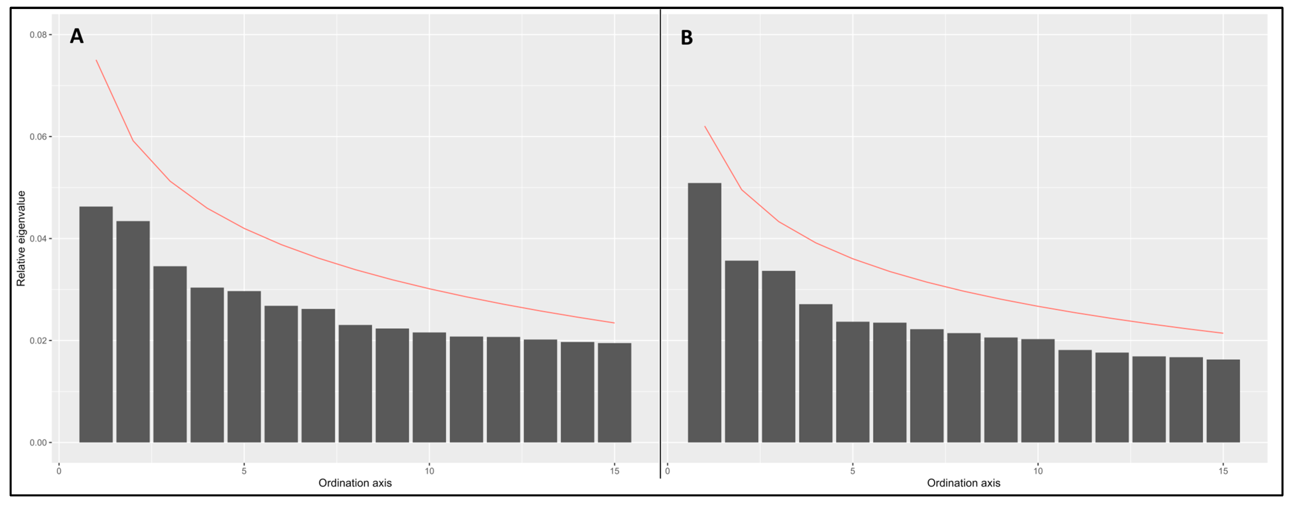
Appendix A.4. Scree Plots Used with the Broken Stick Criterion to Identify the Number of Population Clusters

Figure A3. Scree plots of relative eigenvalues (bars represent real data, the red line represents values from randomly distributed variances) from principal coordinates analyses based on Manhattan distances calculated between individuals in (A) SNP genotype matrix subset for the budburst data and (B) the full SNP genotype matrix.
Forests 16 01233 g0a3

Appendix A.5. Full List of Candidate Loci

Table A2. Full list of candidate loci identified (q < 0.05).
SNP IDChr.Positionq-ValueGene AnnotationDistance from Region (bp)
5738_251149405062.70 × 10−2
52577_2761440191044.89 × 10−3
55616_1891474958364.89 × 10−3Transportin-19254
72253_232263267253.92 × 10−4
83272_1362154790892.10 × 10−2
99516_2912288072263.61 × 10−2
125851_392509705708.53 × 10−4
125860_1042509708246.95 × 10−3
151636_1152725697544.05 × 10−2
164056_792836136368.77 × 10−3
178467_2902953555122.70 × 10−2
178464_1312953556014.96 × 10−2
224662_2853373317228.43 × 10−4Small nucleolar RNA R714392
238225_543491718434.43 × 10−2
262970_683683890613.37 × 10−2
277265_3154126992483.32 × 10−2
305538_1434362558834.43 × 10−2
305941_994363024912.10 × 10−2
316704_2784440959023.37 × 10−2
353121_3104733887112.70 × 10−2
428204_3595537937091.99 × 10−2
457620_635779779484.43 × 10−2Uncharacterised LOC1267272371582
540005_335737879573.37 × 10−2Uncharacterised protein LOC12669180813,272
614926_2848153235613.54 × 10−2(−)-Germacrene D synthase-like164
642304_1348386356007.06 × 10−3
645982_1128416898452.10 × 10−2
690066_2879110146348.77 × 10−3
693924_2879137413923.57 × 10−2rRNA 2′-O-methyltransferase fibrillarin 1-like6951
743550_3231019282273.55 × 10−2
751799_2341088939092.75 × 10−3
765481_23910204692632.70 × 10−2
773508_33010277093482.75 × 10−3
773518_37610277181612.70 × 10−2
775537_30310294360142.75 × 10−3
806456_1810536741732.18 × 10−2
809500_107111548451.87 × 10−2
809532_101111589442.12 × 10−2
837643_21911248967752.29 × 10−2MADS-box protein JOINTLESS-like19,473
861794_14211458312673.57 × 10−2
920002_28512390369223.37 × 10−2
39587_3201329024972.16 × 10−2
50170_231418441571.29 × 10−2
52095_311435841073.84 × 10−2Mediator of RNA polymerase II transcription subunit 251163
88039_542196349567.76 × 10−3
99805_3062290292082.81 × 10−3
185314_48337986491.10 × 10−2
269438_43453482392.81 × 10−3
276966_1424125168642.77 × 10−2Uncharacterized LOC126721394184
277111_324125990173.21 × 10−3Uncharacterized LOC1267205977172
277235_1944126858086.41 × 10−8G-type lectin S-receptor-like serine/threonine-protein kinase At1G6752017,139
277259_1484126990733.83 × 10−7
277265_3154126992481.51 × 10−7
277258_1194126993372.81 × 10−3
277268_1344127000241.52 × 10−7
277302_934127202412.74 × 10−10
318247_2774451764492.57 × 10−5
318272_164451805451.15 × 10−4
318285_3084451828342.60 × 10−3
355472_2754752984096.57 × 10−3Putative disease resistance RPP13-like protein 10
396880_165257812481.96 × 10−2
398425_2135270870392.81 × 10−3
448915_315706610841.71 × 10−2
449028_6 5707664395.62 × 10−6Putative calcium-transporting ATPase 13, plasma membrane-type4865
500170_1496242505694.04 × 10−2
525417_3416464524863.84 × 10−2
526007_1956469110211.81 × 10−2
526011_1066469110561.81 × 10−2
614447_2858150385581.92 × 10−2
614462_2488150394083.34 × 10−4
614940_708153363822.18 × 10−3(−)-Germacrene D synthase-like12,985
621412_2648207758603.79 × 10−2
631293_238295702664.22 × 10−2
663736_1028560303876.57 × 10−3
678922_28491480312.50 × 10−2
693321_2119133680393.84 × 10−2
732227_1979479104121.71 × 10−2
742782_1271011766901.10 × 10−2
745733_61035661184.03 × 10−2
751799_2341088939094.16 × 10−2
766837_28810216652733.48 × 10−2
773466_21310276733633.73 × 10−2
784637_28510365900514.26 × 10−2
810514_104119785733.79 × 10−2
822414_5111115973396.57 × 10−3
840143_19011268740776.29 × 10−3
846236_27111319181012.81 × 10−3Vacuolar-sorting receptor 3-like15,453
884916_1491285172253.70 × 10−2

References

  1. Körner, C.; Möhl, P.; Hiltbrunner, E. Four Ways to Define the Growing Season. Ecol. Lett. 2023, 26, 1277–1292. [Google Scholar] [CrossRef]
  2. Chuine, I. Why Does Phenology Drive Species Distribution? Philos. Trans. R. Soc. B Biol. Sci. 2010, 365, 3149–3160. [Google Scholar] [CrossRef]
  3. Kollas, C.; Körner, C.; Randin, C.F. Spring Frost and Growing Season Length Co-Control the Cold Range Limits of Broad-Leaved Trees. J. Biogeogr. 2014, 41, 773–783. [Google Scholar] [CrossRef]
  4. Körner, C.; Basler, D.; Hoch, G.; Kollas, C.; Lenz, A.; Randin, C.F.; Vitasse, Y.; Zimmermann, N.E. Where, Why and How? Explaining the Low-Temperature Range Limits of Temperate Tree Species. J. Ecol. 2016, 104, 1076–1088. [Google Scholar] [CrossRef]
  5. Jump, A.S.; Peñuelas, J. Running to Stand Still: Adaptation and the Response of Plants to Rapid Climate Change. Ecol. Lett. 2005, 8, 1010–1020. [Google Scholar] [CrossRef]
  6. Jeong, S.-J.; Ho, C.-H.; Gim, H.-J.; Brown, M.E. Phenology Shifts at Start vs. End of Growing Season in Temperate Vegetation over the Northern Hemisphere for the Period 1982–2008. Glob. Change Biol. 2011, 17, 2385–2399. [Google Scholar] [CrossRef]
  7. Piao, S.; Liu, Q.; Chen, A.; Janssens, I.A.; Fu, Y.; Dai, J.; Liu, L.; Lian, X.; Shen, M.; Zhu, X. Plant Phenology and Global Climate Change: Current Progresses and Challenges. Glob. Change Biol. 2019, 25, 1922–1940. [Google Scholar] [CrossRef]
  8. Davis, M.B.; Shaw, R.G. Range Shifts and Adaptive Responses to Quaternary Climate Change. Science 2001, 292, 673–679. [Google Scholar] [CrossRef]
  9. Trew, B.T.; Maclean, I.M. Vulnerability of Global Biodiversity Hotspots to Climate Change. Glob. Ecol. Biogeogr. 2021, 30, 768–783. [Google Scholar] [CrossRef]
  10. Aitken, S.N.; Yeaman, S.; Holliday, J.A.; Wang, T.; Curtis-McLane, S. Adaptation, Migration or Extirpation: Climate Change Outcomes for Tree Populations. Evol. Appl. 2008, 1, 95–111. [Google Scholar] [CrossRef]
  11. Basler, D.; Körner, C. Photoperiod Sensitivity of Bud Burst in 14 Temperate Forest Tree Species. Agric. For. Meteorol. 2012, 165, 73–81. [Google Scholar] [CrossRef]
  12. Basler, D.; Körner, C. Photoperiod and Temperature Responses of Bud Swelling and Bud Burst in Four Temperate Forest Tree Species. Tree Physiol. 2014, 34, 377–388. [Google Scholar] [CrossRef]
  13. Kuster, T.M.; Dobbertin, M.; Günthardt-Goerg, M.S.; Schaub, M.; Arend, M. A Phenological Timetable of Oak Growth under Experimental Drought and Air Warming. PLoS ONE 2014, 9, e89724. [Google Scholar] [CrossRef]
  14. Morin, X.; Roy, J.; Sonié, L.; Chuine, I. Changes in Leaf Phenology of Three European Oak Species in Response to Experimental Climate Change. New Phytol. 2010, 186, 900–910. [Google Scholar] [CrossRef]
  15. Laube, J.; Sparks, T.H.; Estrella, N.; Menzel, A. Does Humidity Trigger Tree Phenology? Proposal for an Air Humidity Based Framework for Bud Development in Spring. New Phytol. 2014, 202, 350–355. [Google Scholar] [CrossRef]
  16. Murray, M.; Smith, R.; Leith, I.; Fowler, D.; Lee, H.; Friend, A.; Jarvis, P. Effects of Elevated CO2, Nutrition and Climatic Warming on Bud Phenology in Sitka Spruce (Picea Sitchensis) and Their Impact on the Risk of Frost Damage. Tree Physiol. 1994, 14, 691–706. [Google Scholar] [CrossRef]
  17. Norby, R.J.; Hartz-Rubin, J.S.; Verbrugge, M.J. Phenological Responses in Maple to Experimental Atmospheric Warming and CO₂ Enrichment. Glob. Change Biol. 2003, 9, 1792–1801. [Google Scholar] [CrossRef]
  18. Vitasse, Y.; Hoch, G.; Randin, C.F.; Lenz, A.; Kollas, C.; Scheepens, J.; Körner, C. Elevational Adaptation and Plasticity in Seedling Phenology of Temperate Deciduous Tree Species. Oecologia 2013, 171, 663–678. [Google Scholar] [CrossRef]
  19. Vitasse, Y.; Porté, A.J.; Kremer, A.; Michalet, R.; Delzon, S. Responses of Canopy Duration to Temperature Changes in Four Temperate Tree Species: Relative Contributions of Spring and Autumn Leaf Phenology. Oecologia 2009, 161, 187–198. [Google Scholar] [CrossRef]
  20. Estiarte, M.; Peñuelas, J. Alteration of the Phenology of Leaf Senescence and Fall in Winter Deciduous Species by Climate Change: Effects on Nutrient Proficiency. Glob. Change Biol. 2015, 21, 1005–1017. [Google Scholar] [CrossRef]
  21. Delpierre, N.; Vitasse, Y.; Chuine, I.; Guillemot, J.; Bazot, S.; Rutishauser, T.; Rathgeber, C.B. Temperate and Boreal Forest Tree Phenology: From Organ-Scale Processes to Terrestrial Ecosystem Models. Ann. For. Sci. 2016, 73, 5–25. [Google Scholar] [CrossRef]
  22. Estrella, N.; Menzel, A. Responses of Leaf Colouring in Four Deciduous Tree Species to Climate and Weather in Germany. Clim. Res. 2006, 32, 253–267. [Google Scholar] [CrossRef]
  23. Mutz, J.; McClory, R.; van Dijk, L.J.; Ehrlén, J.; Tack, A.J. Pathogen Infection Influences the Relationship between Spring and Autumn Phenology at the Seedling and Leaf Level. Oecologia 2021, 197, 447–457. [Google Scholar] [CrossRef]
  24. Delpierre, N.; Guillemot, J.; Dufrêne, E.; Cecchini, S.; Nicolas, M. Tree Phenological Ranks Repeat from Year to Year and Correlate with Growth in Temperate Deciduous Forests. Agric. For. Meteorol. 2017, 234, 1–10. [Google Scholar] [CrossRef]
  25. Crawley, M.; Akhteruzzaman, M. Individual Variation in the Phenology of Oak Trees and Its Consequences for Herbivorous Insects. Funct. Ecol. 1988, 2, 409–415. [Google Scholar] [CrossRef]
  26. Zohner, C.M.; Renner, S.S. Ongoing Seasonally Uneven Climate Warming Leads to Earlier Autumn Growth Cessation in Deciduous Trees. Oecologia 2019, 189, 549–561. [Google Scholar] [CrossRef]
  27. Zohner, C.M.; Mirzagholi, L.; Renner, S.S.; Mo, L.; Rebindaine, D.; Bucher, R.; Palouš, D.; Vitasse, Y.; Fu, Y.H.; Stocker, B.D.; et al. Effect of Climate Warming on the Timing of Autumn Leaf Senescence Reverses after the Summer Solstice. Science 2023, 381, eadf5098. [Google Scholar] [CrossRef]
  28. Bennie, J.; Kubin, E.; Wiltshire, A.; Huntley, B.; Baxter, R. Predicting Spatial and Temporal Patterns of Bud-Burst and Spring Frost Risk in North-West Europe: The Implications of Local Adaptation to Climate. Glob. Change Biol. 2010, 16, 1503–1514. [Google Scholar] [CrossRef]
  29. Baumgarten, F.; Gessler, A.; Vitasse, Y. No Risk—No Fun: Penalty and Recovery from Spring Frost Damage in Deciduous Temperate Trees. Funct. Ecol. 2023, 37, 648–663. [Google Scholar] [CrossRef]
  30. Zohner, C.M.; Mo, L.; Renner, S.S.; Svenning, J.-C.; Vitasse, Y.; Benito, B.M.; Ordonez, A.; Baumgarten, F.; Bastin, J.-F.; Sebald, V.; et al. Late-Spring Frost Risk between 1959 and 2017 Decreased in North America but Increased in Europe and Asia. Proc. Natl. Acad. Sci. USA 2020, 117, 12192–12200. [Google Scholar] [CrossRef]
  31. Augspurger, C.K. Reconstructing Patterns of Temperature, Phenology, and Frost Damage over 124 Years: Spring Damage Risk Is Increasing. Ecology 2013, 94, 41–50. [Google Scholar] [CrossRef]
  32. Bert, D.; Lasnier, J.-B.; Capdevielle, X.; Dugravot, A.; Desprez-Loustau, M.-L. Powdery Mildew Decreases the Radial Growth of Oak Trees with Cumulative and Delayed Effects over Years. PLoS ONE 2016, 11, e0155344. [Google Scholar] [CrossRef]
  33. Pearse, I.S.; Funk, K.A.; Kraft, T.S.; Koenig, W.D. Lagged Effects of Early-Season Herbivores on Valley Oak Fecundity. Oecologia 2015, 178, 361–368. [Google Scholar] [CrossRef]
  34. Renner, S.S.; Zohner, C.M. Climate Change and Phenological Mismatch in Trophic Interactions among Plants, Insects, and Vertebrates. Annu. Rev. Ecol. Evol. Syst. 2018, 49, 165–182. [Google Scholar] [CrossRef]
  35. Gallinat, A.S.; Primack, R.B.; Wagner, D.L. Autumn, the Neglected Season in Climate Change Research. Trends Ecol. Evol. 2015, 30, 169–176. [Google Scholar] [CrossRef]
  36. Alberto, F.; Bouffier, L.; Louvet, J.-M.; Lamy, J.-B.; Delzon, S.; Kremer, A. Adaptive Responses for Seed and Leaf Phenology in Natural Populations of Sessile Oak along an Altitudinal Gradient. J. Evol. Biol. 2011, 24, 1442–1454. [Google Scholar] [CrossRef]
  37. Baliuckas, V.; Pliura, A. Genetic Variation and Phenotypic Plasticity of Quercus Robur Populations and Open-Pollinated Families in Lithuania. Scand. J. For. Res. 2003, 18, 305–319. [Google Scholar] [CrossRef]
  38. Mousseau, T.A. Intra- and Interpopulation Genetic Variation. In Adaptive Genetic Variation in the Wild; Mousseau, T.A., Sinervo, B., Endler, J.A., Eds.; Oxford University Press: New York, NY, USA, 2000; pp. 219–250. [Google Scholar]
  39. Sork, V.L.; Stowe, K.A.; Hochwender, C. Evidence for Local Adaptation in Closely Adjacent Subpopulations of Northern Red Oak (Quercus rubra L.) Expressed as Resistance to Leaf Herbivores. Am. Nat. 1993, 142, 928–936. [Google Scholar] [CrossRef]
  40. Bartholomé, J.; Brachi, B.; Marçais, B.; Mougou-Hamdane, A.; Bodénès, C.; Plomion, C.; Robin, C.; Desprez-Loustau, M.-L. The Genetics of Exapted Resistance to Two Exotic Pathogens in Pedunculate Oak. New Phytol. 2020, 226, 1088–1103. [Google Scholar] [CrossRef]
  41. Carmona, D.; Lajeunesse, M.J.; Johnson, M.T. Plant Traits That Predict Resistance to Herbivores. Funct. Ecol. 2011, 25, 358–367. [Google Scholar] [CrossRef]
  42. Lesur, I.; Le Provost, G.; Bento, P.; Da Silva, C.; Leplé, J.-C.; Murat, F.; Ueno, S.; Bartholomé, J.; Lalanne, C.; Ehrenmann, F.; et al. The Oak Gene Expression Atlas: Insights into Fagaceae Genome Evolution and the Discovery of Genes Regulated during Bud Dormancy Release. BMC Genom. 2015, 16, 112. [Google Scholar] [CrossRef]
  43. Derory, J.; Léger, P.; Garcia, V.; Schaeffer, J.; Hauser, M.-T.; Salin, F.; Luschnig, C.; Plomion, C.; Glössl, J.; Kremer, A. Transcriptome Analysis of Bud Burst in Sessile Oak (Quercus petraea). New Phytol. 2006, 170, 723–738. [Google Scholar] [CrossRef]
  44. Derory, J.; Scotti-Saintagne, C.; Bertocchi, E.; Le Dantec, L.; Graignic, N.; Jauffres, A.; Casasoli, M.; Chancerel, E.; Bodénès, C.; Alberto, F.; et al. Contrasting Relationships between the Diversity of Candidate Genes and Variation of Bud Burst in Natural and Segregating Populations of European Oaks. Heredity 2010, 104, 438–448. [Google Scholar] [CrossRef]
  45. Alberto, F.J.; Derory, J.; Boury, C.; Frigerio, J.-M.; Zimmermann, N.E.; Kremer, A. Imprints of Natural Selection along Environmental Gradients in Phenology-Related Genes of Quercus petraea. Genetics 2013, 195, 495–512. [Google Scholar] [CrossRef]
  46. Diekmann, M. Deciduous Forest Vegetation in Boreo-Nemoral Scandinavia. Ph.D. Thesis, Uppsala University, Uppsala, Sweden, 1994. [Google Scholar]
  47. Vranckx, G.; Jacquemyn, H.; Mergeay, J.; Cox, K.; Kint, V.; Muys, B.; Honnay, O. Transmission of Genetic Variation from the Adult Generation to Naturally Established Seedling Cohorts in Small Forest Stands of Pedunculate Oak (Quercus robur L.). For. Ecol. Manag. 2014, 312, 19–27. [Google Scholar] [CrossRef]
  48. Moracho, E.; Moreno, G.; Jordano, P.; Hampe, A. Unusually Limited Pollen Dispersal and Connectivity of Pedunculate Oak (Quercus robur) Refugial Populations at the Species’ Southern Range Margin. Mol. Ecol. 2016, 25, 3319–3331. [Google Scholar] [CrossRef]
  49. Buschbom, J.; Yanbaev, Y.; Degen, B. Efficient Long-Distance Gene Flow into an Isolated Relict Oak Stand. J. Hered. 2011, 102, 464–472. [Google Scholar] [CrossRef]
  50. Eaton, E.; Caudullo, G.; Oliveira, S.; de Rigo, D. Quercus Robur and Quercus Petraea in Europe: Distribution, Habitat, Usage and Threats. In European Atlas of Forest Tree Species; San-Miguel-Ayanz, J., de Rigo, D., Caudullo, G., Houston Durrant, T., Mauri, A., Eds.; Publications Office of the EU: Luxembourg, 2016; p. e01c6df+. [Google Scholar]
  51. Sunde, J.; Franzén, M.; Betzholtz, P.-E.; Francioli, Y.; Pettersson, L.B.; Pöyry, J.; Ryrholm, N.; Forsman, A. Century-Long Butterfly Range Expansions in Northern Europe Depend on Climate, Land Use and Species Traits. Commun. Biol. 2023, 6, 601. [Google Scholar] [CrossRef]
  52. Forsman, A.; Sunde, J.; Salis, R.; Franzén, M. Latitudinal Gradients of Biodiversity and Ecosystem Services in Protected and Non-Protected Oak Forest Areas Can Inform Climate Smart Conservation. Geogr. Sustain. 2024, 5, 647–659. [Google Scholar] [CrossRef]
  53. Hall, M.; Franzén, M.; Forsman, A.; Sunde, J. Spatially Varying Selection and Contrasting Patterns in Neutral and Adaptive Genetic Variation towards the Cold-Limited Northern Range Margin in Quercus Robur. Submitt. Evol. Appl. 2025. [Google Scholar]
  54. Black-Samuelsson, S. Den Skogliga Genbanken—Från Storhetstid Till Framtid; Skogsstyrelsen: Jönköping, Sweden, 2019. [Google Scholar]
  55. Johansson, V.; Forsman, A.; Gustafsson, L.; Hall, M.; Edvardsson, J.; Salis, R.; Sunde, J.; Franzén, M. Low Cross-Taxon Congruence and Weak Stand-Age Effects on Biodiversity in Swedish Oak Forests. Biodivers. Conserv. 2025, 34, 2739–2750. [Google Scholar] [CrossRef]
  56. Faticov, M.; Ekholm, A.; Roslin, T.; Tack, A.J. Climate and Host Genotype Jointly Shape Tree Phenology, Disease Levels and Insect Attacks. Oikos 2020, 129, 391–401. [Google Scholar] [CrossRef]
  57. Mariën, B.; Balzarolo, M.; Dox, I.; Leys, S.; Lorène, M.J.; Geron, C.; Portillo-Estrada, M.; AbdElgawad, H.; Asard, H.; Campioli, M. Detecting the Onset of Autumn Leaf Senescence in Deciduous Forest Trees of the Temperate Zone. New Phytol. 2019, 224, 166–176. [Google Scholar] [CrossRef]
  58. Johansson, B. Areal Precipitation and Temperature in the Swedish Mountains: An Evaluation from a Hydrological Perspective. Hydrol. Res. 2000, 31, 207–228. [Google Scholar] [CrossRef]
  59. Brooks, M.E.; Kristensen, K.; van Benthem, K.J.; Magnusson, A.; Berg, C.W.; Nielsen, A.; Skaug, H.J.; Mächler, M.; Bolker, B.M. glmmTMB Balances Speed and Flexibility among Packages for Zero-Inflated Generalized Linear Mixed Modeling. R J. 2017, 9, 378–400. [Google Scholar] [CrossRef]
  60. Weisberg, F.J. An R Companion to Applied Regression, 3rd ed.; Sage: Thousand Oaks, CA, USA, 2019. [Google Scholar]
  61. Bartoń, K. “MuMIn”: Multi-Model Inference 2025. Available online: https://CRAN.R-project.org/package=MuMIn (accessed on 10 July 2025).
  62. Rochette, N.C.; Rivera-Colón, A.G.; Catchen, J.M. Stacks 2: Analytical Methods for Paired-End Sequencing Improve RADseq-Based Population Genomics. Mol. Ecol. 2019, 28, 4737–4754. [Google Scholar] [CrossRef]
  63. Andrews, S. FastQC: A Quality Control Tool for High Throughput Sequence Data. 2010. Available online: https://www.bioinformatics.babraham.ac.uk/projects/fastqc/ (accessed on 10 July 2025).
  64. Ewels, P.; Magnusson, M.; Lundin, S.; Käller, M. MultiQC: Summarize Analysis Results for Multiple Tools and Samples in a Single Report. Bioinformatics 2016, 32, 3047–3048. [Google Scholar] [CrossRef]
  65. Li, H.; Durbin, R. Fast and Accurate Short Read Alignment with Burrows–Wheeler Transform. Bioinformatics 2009, 25, 1754–1760. [Google Scholar] [CrossRef]
  66. Danecek, P.; Bonfield, J.K.; Liddle, J.; Marshall, J.; Ohan, V.; Pollard, M.O.; Whitwham, A.; Keane, T.; McCarthy, S.A.; Davies, R.M.; et al. Twelve Years of SAMtools and BCFtools. Gigascience 2021, 10, giab008. [Google Scholar] [CrossRef]
  67. Paris, J.R.; Stevens, J.R.; Catchen, J.M. Lost in Parameter Space: A Road Map for Stacks. Methods Ecol. Evol. 2017, 8, 1360–1373. [Google Scholar] [CrossRef]
  68. Purcell, S.; Neale, B.; Todd-Brown, K.; Thomas, L.; Ferreira, M.A.; Bender, D.; Maller, J.; Sklar, P.; De Bakker, P.I.; Daly, M.J.; et al. PLINK: A Tool Set for Whole-Genome Association and Population-Based Linkage Analyses. Am. J. Hum. Genet. 2007, 81, 559–575. [Google Scholar] [CrossRef]
  69. Browning, B.L.; Zhou, Y.; Browning, S.R. A One-Penny Imputed Genome from next-Generation Reference Panels. Am. J. Hum. Genet. 2018, 103, 338–348. [Google Scholar] [CrossRef]
  70. Vitasse, Y.; Bresson, C.C.; Kremer, A.; Michalet, R.; Delzon, S. Quantifying Phenological Plasticity to Temperature in Two Temperate Tree Species. Funct. Ecol. 2010, 24, 1211–1218. [Google Scholar] [CrossRef]
  71. Kang, H.M.; Zaitlen, N.A.; Wade, C.M.; Kirby, A.; Heckerman, D.; Daly, M.J.; Eskin, E. Efficient Control of Population Structure in Model Organism Association Mapping. Genetics 2008, 178, 1709–1723. [Google Scholar] [CrossRef]
  72. Lin, J.; Berveiller, D.; François, C.; Hänninen, H.; Morfin, A.; Vincent, G.; Zhang, R.; Rathgeber, C.; Delpierre, N. A Model of the Within-Population Variability of Budburst in Forest Trees. Geosci. Model Dev. 2024, 17, 865–879. [Google Scholar] [CrossRef]
  73. Frontiér, S. Étude de La Décroissance Des Valeurs Propres Dans Une Analyse En Composantes Principales: Comparaison Avec Le Modéle Du Batôn Brisé. J. Exp. Mar. Biol. Ecol. 1976, 25, 67–75. [Google Scholar] [CrossRef]
  74. Jackson, D.A. Stopping Rules in Principal Components Analysis: A Comparison of Heuristical and Statistical Approaches. Ecology 1993, 74, 2204–2214. [Google Scholar] [CrossRef]
  75. Cattell, R.B. The Scree Test for the Number of Factors. Multivar. Behav. Res. 1966, 1, 245–276. [Google Scholar] [CrossRef]
  76. Raj, A.; Stephens, M.; Pritchard, J.K. fastSTRUCTURE: Variational Inference of Population Structure in Large SNP Data Sets. Genetics 2014, 197, 573–589. [Google Scholar] [CrossRef]
  77. Hamilton, M.B. Population Genetics; Wiley-Blackwell: Hoboken, NJ, USA, 2009. [Google Scholar]
  78. Zhang, C.; Dong, S.-S.; Xu, J.-Y.; He, W.-M.; Yang, T.-L. PopLDdecay: A Fast and Effective Tool for Linkage Disequilibrium Decay Analysis Based on Variant Call Format Files. Bioinformatics 2019, 35, 1786–1788. [Google Scholar] [CrossRef]
  79. Otyama, P.I.; Wilkey, A.; Kulkarni, R.; Assefa, T.; Chu, Y.; Clevenger, J.; O’Connor, D.J.; Wright, G.C.; Dezern, S.W.; MacDonald, G.E.; et al. Evaluation of Linkage Disequilibrium, Population Structure, and Genetic Diversity in the US Peanut Mini Core Collection. BMC Genom. 2019, 20, 481. [Google Scholar] [CrossRef]
  80. Pang, Y.; Liu, C.; Wang, D.; Amand, P.S.; Bernardo, A.; Li, W.; He, F.; Li, L.; Wang, L.; Yuan, X.; et al. High-Resolution Genome-Wide Association Study Identifies Genomic Regions and Candidate Genes for Important Agronomic Traits in Wheat. Mol. Plant 2020, 13, 1311–1327. [Google Scholar] [CrossRef]
  81. Legendre, P.; Legendre, L. Numerical Ecology, 3rd ed.; Elsevier B.V.: Oxford, UK, 2012. [Google Scholar]
  82. Forester, B.R.; Lasky, J.R.; Wagner, H.H.; Urban, D.L. Comparing Methods for Detecting Multilocus Adaptation with Multivariate Genotype–Environment Associations. Mol. Ecol. 2018, 27, 2215–2233. [Google Scholar] [CrossRef]
  83. Le Corre, V.; Kremer, A. The Genetic Differentiation at Quantitative Trait Loci under Local Adaptation. Mol. Ecol. 2012, 21, 1548–1566. [Google Scholar] [CrossRef]
  84. Kremer, A.; Le Corre, V.; Petit, R.J.; Ducousso, A. Historical and Contemporary Dynamics of Adaptive Differentiation in European Oaks. In Molecular Approaches in Natural Resource Conservation and Management; DeWoody, J., Bickham, J., Michler, C., Nichols, K., Rhodes, G., Woeste, K., Eds.; Cambridge University Press: Cambridge, UK, 2010; pp. 101–122. [Google Scholar]
  85. Oksanen, J.; Simpson, G.; Blanchet, F.; Kindt, R.; Legendre, P.; Minchin, P.; O’Hara, R.; Solymos, P.; Stevens, M.; Szoecs, E.; et al. Vegan: Community Ecology Package. 2022. Available online: https://CRAN.R-project.org/package=vegan (accessed on 10 July 2025).
  86. Storey, J.D.; Bass, A.J.; Dabney, A.; Robinson, D. Qvalue: Q-Value Estimation for False Discovery Rate Control. 2023. Available online: https://www.bioconductor.org/packages/devel/bioc/manuals/qvalue/man/qvalue.pdf (accessed on 21 July 2025).
  87. Wickham, H. Ggplot2: Elegant Graphics for Data Analysis; Springer-Verlag: New York, NY, USA, 2016. [Google Scholar]
  88. Bodénès, C.; Chancerel, E.; Ehrenmann, F.; Kremer, A.; Plomion, C. High-Density Linkage Mapping and Distribution of Segregation Distortion Regions in the Oak Genome. DNA Res. 2016, 23, 115–124. [Google Scholar] [CrossRef]
  89. Excoffier, L.; Smouse, P.E.; Quattro, J.M. Analysis of Molecular Variance Inferred from Metric Distances among DNA Haplotypes: Application to Human Mitochondrial DNA Restriction Data. Genetics 1992, 131, 479–491. [Google Scholar] [CrossRef]
  90. Paradis, E. Pegas: An R Package for Population Genetics with an Integrated–Modular Approach. Bioinformatics 2010, 26, 419–420. [Google Scholar] [CrossRef]
  91. Holsinger, K.E.; Weir, B.S. Genetics in Geographically Structured Populations: Defining, Estimating and Interpreting FST. Nat. Rev. Genet. 2009, 10, 639–650. [Google Scholar] [CrossRef]
  92. Ziemienowicz, A.; Haasen, D.; Staiger, D.; Merkle, T. Arabidopsis Transportin1 Is the Nuclear Import Receptor for the Circadian Clock-Regulated RNA-Binding Protein AtGRP7. Plant Mol. Biol. 2003, 53, 201–212. [Google Scholar] [CrossRef]
  93. Yan, B.; Wang, X.; Wang, Z.; Chen, N.; Mu, C.; Mao, K.; Han, L.; Zhang, W.; Liu, H. Identification of Potential Cargo Proteins of Transportin Protein AtTRN1 in Arabidopsis thaliana. Plant Cell Rep. 2016, 35, 629–640. [Google Scholar] [CrossRef]
  94. Bhattacharya, D.P. Study of Small Non-Coding RNAs in Plants by Developing Novel Pipelines. Ph.D. Thesis, Universitäts-und Landesbibliothek Sachsen-Anhalt, Halle, Germany, 2017. [Google Scholar]
  95. Osuna-Caballero, S.; Rubiales, D.; Rispail, N. Genome-Wide Association Study Uncovers Pea Candidate Genes and Metabolic Pathways Involved in Rust Resistance. Plant Genome 2024, 17, e20510. [Google Scholar] [CrossRef]
  96. Arimura, G.; Huber, D.P.; Bohlmann, J. Forest Tent Caterpillars (Malacosoma disstria) Induce Local and Systemic Diurnal Emissions of Terpenoid Volatiles in Hybrid Poplar (Populus trichocarpa × Deltoides): cDNA Cloning, Functional Characterization, and Patterns of Gene Expression of (-)-Germacrene D Synthase, PtdTPS1. Plant J. 2004, 37, 603–616. [Google Scholar] [CrossRef]
  97. Muñoz-Diaz, E.; Fuenzalida-Valdivia, I.; Darriere, T.; de Bures, A.; Blanco-Herrera, F.; Rompais, M.; Carapito, C.; Saez-Vasquez, J. Proteomic Profiling of Arabidopsis Nuclei Reveals Distinct Protein Accumulation Kinetics upon Heat Stress. Sci. Rep. 2024, 14, 18914. [Google Scholar] [CrossRef]
  98. Cohen, O.; Borovsky, Y.; David-Schwartz, R.; Paran, I. CaJOINTLESS Is a MADS-Box Gene Involved in Suppression of Vegetative Growth in All Shoot Meristems in Pepper. J. Exp. Bot. 2012, 63, 4947–4957. [Google Scholar] [CrossRef]
  99. Mao, L.; Begum, D.; Chuang, H.; Budiman, M.A.; Szymkowiak, E.J.; Irish, E.E.; Wing, R.A. JOINTLESS Is a MADS-Box Gene Controlling Tomato Flower Abscission Zone Development. Nature 2000, 406, 910–913. [Google Scholar] [CrossRef]
  100. Fernandes, P.M. Molecular and Histological Approaches to Unravel Castanea spp. Responses to Phytophthora cinnamomi Infection. Ph.D. Thesis, Universidade NOVA de Lisboa, Lisbon, Portugal, 2022. [Google Scholar]
  101. Iizasa, S.; Iizasa, E.; Watanabe, K.; Nagano, Y. Transcriptome Analysis Reveals Key Roles of AtLBR-2 in LPS-Induced Defense Responses in Plants. BMC Genom. 2017, 18, 995. [Google Scholar] [CrossRef]
  102. Chandran, N.K.; Sriram, S.; Prakash, T.; Budhwar, R. Transcriptome Changes in Resistant and Susceptible Rose in Response to Powdery Mildew. J. Phytopathol. 2021, 169, 556–569. [Google Scholar] [CrossRef]
  103. Szajko, K.; Sołtys-Kalina, D.; Heidorn-Czarna, M.; Smyda-Dajmund, P.; Wasilewicz-Flis, I.; Jańska, H.; Marczewski, W. Transcriptomic and Proteomic Data Provide New Insights into Cold-Treated Potato Tubers with T-and D-Type Cytoplasm. Planta 2022, 255, 97. [Google Scholar] [CrossRef]
  104. Shen, C.; Shi, X.; Xie, C.; Li, Y.; Yang, H.; Mei, X.; Xu, Y.; Dong, C. The Change in Microstructure of Petioles and Peduncles and Transporter Gene Expression by Potassium Influences the Distribution of Nutrients and Sugars in Pear Leaves and Fruit. J. Plant Physiol. 2019, 232, 320–333. [Google Scholar] [CrossRef]
  105. Fernandes, I.; Paulo, O.S.; Marques, I.; Sarjkar, I.; Sen, A.; Graça, I.; Pawlowski, K.; Ramalho, J.C.; Ribeiro-Barros, A.I. Salt Stress Tolerance in Casuarina Glauca: Insights from the Branchlets Transcriptome. Plants 2022, 11, 2942. [Google Scholar] [CrossRef]
  106. Figueiredo, J.; Santos, R.B.; Guerra-Guimarães, L.; Leclercq, C.C.; Renaut, J.; Sousa, L.; Figueiredo, A. Revealing the Secrets beneath Grapevine and Plasmopara Viticola Early Communication: A Picture of Host and Pathogen Proteomes. bioRxiv 2021, preprint. [Google Scholar] [CrossRef]
  107. Hu, X.; Wu, L.; Zhao, F.; Zhang, D.; Li, N.; Zhu, G.; Li, C.; Wang, W. Phosphoproteomic Analysis of the Response of Maize Leaves to Drought, Heat and Their Combination Stress. Front. Plant Sci. 2015, 6, 298. [Google Scholar] [CrossRef]
  108. Lenz, A.; Hoch, G.; Vitasse, Y.; Körner, C. European Deciduous Trees Exhibit Similar Safety Margins against Damage by Spring Freeze Events along Elevational Gradients. New Phytol. 2013, 200, 1166–1175. [Google Scholar] [CrossRef]
  109. Schaber, J.; Badeck, F.-W. Physiology-Based Phenology Models for Forest Tree Species in Germany. Int. J. Biometeorol. 2003, 47, 193–201. [Google Scholar] [CrossRef]
  110. Zohner, C.M.; Benito, B.M.; Svenning, J.-C.; Renner, S.S. Day Length Unlikely to Constrain Climate-Driven Shifts in Leaf-out Times of Northern Woody Plants. Nat. Clim. Change 2016, 6, 1120–1123. [Google Scholar] [CrossRef]
  111. Dantec, C.F.; Ducasse, H.; Capdevielle, X.; Fabreguettes, O.; Delzon, S.; Desprez-Loustau, M.-L. Escape of Spring Frost and Disease through Phenological Variations in Oak Populations along Elevation Gradients. J. Ecol. 2015, 103, 1044–1056. [Google Scholar] [CrossRef]
  112. Zohner, C.M.; Mo, L.; Sebald, V.; Renner, S.S. Leaf-out in Northern Ecotypes of Wide-Ranging Trees Requires Less Spring Warming, Enhancing the Risk of Spring Frost Damage at Cold Range Limits. Glob. Ecol. Biogeogr. 2020, 29, 1065–1072. [Google Scholar] [CrossRef]
  113. Olsson, C.; Bolmgren, K.; Lindström, J.; Jönsson, A.M. Performance of Tree Phenology Models along a Bioclimatic Gradient in Sweden. Ecol. Model. 2013, 266, 103–117. [Google Scholar] [CrossRef]
  114. Ducousso, A.; Guyon, J.; Krémer, A. Latitudinal and Altitudinal Variation of Bud Burst in Western Populations of Sessile Oak (Quercus petraea (Matt) Liebl). In Proceedings of the Annales des Sciences Forestières; EDP Sciences: Les Ulis, France, 1996; Volume 53, pp. 775–782. [Google Scholar]
  115. Delpierre, N.; Dufrêne, E.; Soudani, K.; Ulrich, E.; Cecchini, S.; Boé, J.; François, C. Modelling Interannual and Spatial Variability of Leaf Senescence for Three Deciduous Tree Species in France. Agric. For. Meteorol. 2009, 149, 938–948. [Google Scholar] [CrossRef]
  116. Mariën, B.; Dox, I.; De Boeck, H.J.; Willems, P.; Leys, S.; Papadimitriou, D.; Campioli, M. Does Drought Advance the Onset of Autumn Leaf Senescence in Temperate Deciduous Forest Trees? Biogeosciences 2021, 18, 3309–3330. [Google Scholar] [CrossRef]
  117. Wang, H.; Gao, C.; Ge, Q. Low Temperature and Short Daylength Interact to Affect the Leaf Senescence of Two Temperate Tree Species. Tree Physiol. 2022, 42, 2252–2265. [Google Scholar] [CrossRef]
  118. Zani, D.; Crowther, T.W.; Mo, L.; Renner, S.S.; Zohner, C.M. Increased Growing-Season Productivity Drives Earlier Autumn Leaf Senescence in Temperate Trees. Science 2020, 370, 1066–1071. [Google Scholar] [CrossRef]
  119. Firmat, C.; Delzon, S.; Louvet, J.-M.; Parmentier, J.; Kremer, A. Evolutionary Dynamics of the Leaf Phenological Cycle in an Oak Metapopulation along an Elevation Gradient. J. Evol. Biol. 2017, 30, 2116–2131. [Google Scholar] [CrossRef]
  120. Desprez-Loustau, M.-L.; Vitasse, Y.; Delzon, S.; Capdevielle, X.; Marais, B.; Kremer, A. Are Plant Pathogen Populations Adapted for Encounter with Their Host? A Case Study of Phenological Synchrony between Oak and an Obligate Fungal Parasite along an Altitudinal Gradient. J. Evol. Biol. 2010, 23, 87–97. [Google Scholar] [CrossRef]
  121. Desprez-Loustau, M.-L.; Saint-Jean, G.; Barrès, B.; Dantec, C.F.; Dutech, C. Oak Powdery Mildew Changes Growth Patterns in Its Host Tree: Host Tolerance Response and Potential Manipulation of Host Physiology by the Parasite. Ann. For. Sci. 2014, 71, 563–573. [Google Scholar] [CrossRef]
  122. Ovaskainen, O.; Laine, A.-L. Inferring Evolutionary Signals from Ecological Data in a Plant–Pathogen Metapopulation. Ecology 2006, 87, 880–891. [Google Scholar] [CrossRef]
  123. Bertić, M.; Schroeder, H.; Kersten, B.; Fladung, M.; Orgel, F.; Buegger, F.; Schnitzler, J.-P.; Ghirardo, A. European Oak Chemical Diversity–from Ecotypes to Herbivore Resistance. New Phytol. 2021, 232, 818–834. [Google Scholar] [CrossRef]
  124. Hunter, M.D. A Variable Insect–Plant Interaction: The Relationship between Tree Budburst Phenology and Population Levels of Insect Herbivores among Trees. Ecol. Entomol. 1992, 17, 91–95. [Google Scholar] [CrossRef]
  125. Wesołowski, T.; Rowiński, P. Late Leaf Development in Pedunculate Oak (Quercus Robur): An Antiherbivore Defence? Scand. J. For. Res. 2008, 23, 386–394. [Google Scholar] [CrossRef]
  126. Ekholm, A.; Tack, A.J.; Bolmgren, K.; Roslin, T. The Forgotten Season: The Impact of Autumn Phenology on a Specialist Insect Herbivore Community on Oak. Ecol. Entomol. 2019, 44, 425–435. [Google Scholar] [CrossRef]
  127. Valdés-Correcher, E.; Kadiri, Y.; Bourdin, A.; Mrazova, A.; Bălăcenoiu, F.; Branco, M.; Bogdziewicz, M.; Bjørn, M.C.; Damestoy, T.; Dobrosavljević, J.; et al. Effects of Climate on Leaf Phenolics, Insect Herbivory, and Their Relationship in Pedunculate Oak (Quercus Robur) across Its Geographic Range in Europe. Oecologia 2025, 207, 61. [Google Scholar] [CrossRef]
  128. Čehulić, I.; Sever, K.; Katičić Bogdan, I.; Jazbec, A.; Škvorc, Ž.; Bogdan, S. Drought Impact on Leaf Phenology and Spring Frost Susceptibility in a Quercus Robur L. Provenance Trial. Forests 2019, 10, 50. [Google Scholar] [CrossRef]
  129. Vander Mijnsbrugge, K.; Turcsán, A.; Maes, J.; Duchêne, N.; Meeus, S.; Steppe, K.; Steenackers, M. Repeated Summer Drought and Re-Watering during the First Growing Year of Oak (Quercus petraea) Delay Autumn Senescence and Bud Burst in the Following Spring. Front. Plant Sci. 2016, 7, 419. [Google Scholar] [CrossRef]
  130. Misson, L.; Limousin, J.-M.; Rodriguez, R.; Letts, M.G. Leaf Physiological Responses to Extreme Droughts in Mediterranean Quercus Ilex Forest. Plant Cell Environ. 2010, 33, 1898–1910. [Google Scholar] [CrossRef]
  131. Misson, L.; Degueldre, D.; Collin, C.; Rodriguez, R.; Rocheteau, A.; Ourcival, J.-M.; Rambal, S. Phenological Responses to Extreme Droughts in a Mediterranean Forest. Glob. Change Biol. 2011, 17, 1036–1048. [Google Scholar] [CrossRef]
  132. Bréda, N.; Badeau, V. Forest Tree Responses to Extreme Drought and Some Biotic Events: Towards a Selection According to Hazard Tolerance? Comptes Rendus Géoscience 2008, 340, 651–662. [Google Scholar] [CrossRef]
  133. Bose, A.K.; Scherrer, D.; Camarero, J.J.; Ziche, D.; Babst, F.; Bigler, C.; Bolte, A.; Dorado-Liñán, I.; Etzold, S.; Fonti, P.; et al. Climate Sensitivity and Drought Seasonality Determine Post-Drought Growth Recovery of Quercus petraea and Quercus robur in Europe. Sci. Total Environ. 2021, 784, 147222. [Google Scholar] [CrossRef]
  134. Grossman, J.J. Phenological Physiology: Seasonal Patterns of Plant Stress Tolerance in a Changing Climate. New Phytol. 2023, 237, 1508–1524. [Google Scholar] [CrossRef]
  135. Koenig, W.D.; Funk, K.A.; Kraft, T.S.; Carmen, W.J.; Barringer, B.C.; Knops, J.M. Stabilizing Selection for Within-Season Flowering Phenology Confirms Pollen Limitation in a Wind-Pollinated Tree. J. Ecol. 2012, 100, 758–763. [Google Scholar] [CrossRef]
  136. Ismail, S.A.; Kokko, H. An Analysis of Mating Biases in Trees. Mol. Ecol. 2020, 29, 184–198. [Google Scholar] [CrossRef]
  137. Alberto, F.J.; Aitken, S.N.; Alía, R.; González-Martínez, S.C.; Hänninen, H.; Kremer, A.; Lefèvre, F.; Lenormand, T.; Yeaman, S.; Whetten, R.; et al. Potential for Evolutionary Responses to Climate Change–Evidence from Tree Populations. Glob. Change Biol. 2013, 19, 1645–1661. [Google Scholar] [CrossRef]
  138. Rellstab, C.; Gugerli, F.; Eckert, A.J.; Hancock, A.M.; Holderegger, R. A Practical Guide to Environmental Association Analysis in Landscape Genomics. Mol. Ecol. 2015, 24, 4348–4370. [Google Scholar] [CrossRef]
  139. Hewitt, G. The Genetic Legacy of the Quaternary Ice Ages. Nature 2000, 405, 907–913. [Google Scholar] [CrossRef]
  140. Kremer, A.; Hipp, A.L. Oaks: An Evolutionary Success Story. New Phytol. 2020, 226, 987–1011. [Google Scholar] [CrossRef]
  141. Gerber, S.; Chadøeuf, J.; Gugerli, F.; Lascoux, M.; Buiteveld, J.; Cottrell, J.; Dounavi, A.; Fineschi, S.; Forrest, L.L.; Fogelqvist, J.; et al. High Rates of Gene Flow by Pollen and Seed in Oak Populations across Europe. PLoS ONE 2014, 9, e85130. [Google Scholar] [CrossRef]
  142. Slatkin, M. Gene Flow and the Geographic Structure of Natural Populations. Science 1987, 236, 787–792. [Google Scholar] [CrossRef]
  143. Pringle, J.M.; Wares, J.P. Going against the Flow: Maintenance of Alongshore Variation in Allele Frequency in a Coastal Ocean. Mar. Ecol. Prog. Ser. 2007, 335, 69–84. [Google Scholar] [CrossRef]
  144. Koski, V. A Study of Pollen Dispersal as a Mechanism of Gene Flow in Conifers. Commun. Inst. For. Fenn. 1970, 70, 78. [Google Scholar]
  145. Persson, B.; Ståhl, E.G. Survival and Yield of Pinus Sylvestris L. as Related to Provenance Transfer and Spacing at High Altitudes in Northern Sweden. Scand. J. For. Res. 1990, 5, 381–395. [Google Scholar] [CrossRef]
  146. Dalongeville, A.; Andrello, M.; Mouillot, D.; Lobreaux, S.; Fortin, M.-J.; Lasram, F.; Belmaker, J.; Rocklin, D.; Manel, S. Geographic Isolation and Larval Dispersal Shape Seascape Genetic Patterns Differently According to Spatial Scale. Evol. Appl. 2018, 11, 1437–1447. [Google Scholar] [CrossRef]
  147. Kleinschmit, J. Intraspecific Variation of Growth and Adaptive Traits in European Oak Species. Ann. Des Sci. For. 1993, 50, 166–185. [Google Scholar] [CrossRef]
  148. Eckert, C.G.; Samis, K.E.; Lougheed, S.C. Genetic Variation across Species’ Geographical Ranges: The Central–Marginal Hypothesis and Beyond. Mol. Ecol. 2008, 17, 1170–1188. [Google Scholar] [CrossRef]
  149. Templ, B.; Koch, E.; Bolmgren, K.; Ungersböck, M.; Paul, A.; Scheifinger, H.; Rutishauser, T.; Busto, M.; Chmielewski, F.-M.; Hájková, L.; et al. Pan European Phenological Database (PEP725): A Single Point of Access for European Data. Int. J. Biometeorol. 2018, 62, 1109–1113. [Google Scholar] [CrossRef]
  150. Chau, J. Gslnls: GSL Nonlinear Least-Squares Fitting 2023. Available online: https://CRAN.R-project.org/package=gslnls (accessed on 10 July 2025).
  151. R Core Team. R: A Language and Environment for Statistical Computing 2023; R Foundation for Statistical Computing: Vienna, Austria, 2023; Available online: https://www.R-project.org/ (accessed on 10 July 2025).
  152. Kikuchi, S.; Bheemanahalli, R.; Jagadish, K.S.; Kumagai, E.; Masuya, Y.; Kuroda, E.; Raghavan, C.; Dingkuhn, M.; Abe, A.; Shimono, H. Genome-Wide Association Mapping for Phenotypic Plasticity in Rice. Plant Cell Environ. 2017, 40, 1565–1575. [Google Scholar] [CrossRef]
Figure 1. (A) Map of stand locations. Attributions for the basemaps: Esri, DigitalGlobe, GeoEye, i-cubed, USDA FSA, USGS, AEX, Getmapping, Aerogrid, IGN, IGP, swisstopo, the GIS User Community, DeLorme, HERE, and MapmyIndia; (B) Photographs of each stage of leaf unfolding, as described in the text. All photographs were taken by Isaksson, J.; (C) and (D) boxplots of budburst and leaf senescence onset dates, respectively.
Forests 16 01233 g001
Figure 2. Manhattan plots of SNPs and q-values from association tests with standardised timings (panel (A) is budburst; panel (B) is leaf senescence). Points with colours other than grey are loci with q-values lower than 0.05, the chosen significance level. Orange and green indicate loci located within 20 kbp of a putatively coding region in the annotated genome, either with a described (orange) or uncharacterised (green) function; while purple indicates significant loci located more than 20 kbp from the closest putatively coding region in the annotated genome. SNPs are ordered by chromosome and location, with the exception of the second rightmost section (Pltd), where SNPs came from chloroplast genome, and the rightmost section (Shotgun), which contains SNPs from an unlocalised scaffold of contigs from chromosome 7.
Forests 16 01233 g002
Figure 3. Pairwise genetic differentiation between stands in the full dataset (green), the candidate locus dataset associated with relative budburst (blue), and the candidate locus dataset associated with relative leaf senescence (red). Stands are ordered by latitude.
Forests 16 01233 g003
Table 1. Results from individual linear mixed models were used to test for associations between the timing of phenological events and drivers. “April temp.” and “August temp.” represent the mean daily temperatures (°C) during the months of April and August, respectively. Given are a χ2-statistic from a Type 2 Wald test of the variable, regression coefficients (Est.), p-values associated with the χ2-statistics, and marginal and conditional R2 values (R2M and R2C, respectively).
χ2Est.p-ValueR2MR2C
BudburstApril temp.7.55−2.890.0010.360.79
Latitude3.901.300.0480.240.79
Leaf senescenceBudburst0.180.210.670.010.34
August temp.3.6010.380.060.110.32
Latitude10.73−3.420.0010.210.32
Table 2. Functions of significant SNPs (q-values < 0.05) also found in the annotated genome for Quercus robur (L.). For each locus, its SNP ID in the full RADseq dataset, chromosome number (Chr.), position on the chromosome, significance (q-value), name of the previously associated function, a short description of the function in other organisms, and the distance from the region are given. Candidate loci associated with relative budburst are above the dividing line, and ones below were associated with relative leaf senescence.
SNP IDChr.Positionq-ValueGene AnnotationPossibly Associated withDistance from Region (bp)
55616_189 1474958364.89 × 10−3Transportin-1Several
functions
9254
224662_2853373317228.43 × 10−4Small nucleolar RNA R71Pathogen
defence
4392
614926_2848153235613.54 × 10−2(−)-Germacrene D synthase-likeHerbivory
defence
164
693924_2879137413923.57 × 10−2rRNA 2′-O-methyltransferase
serine/threonine-fibrillarin 1-like
Heat stress
recovery
6951
837643_21911248967752.29 × 10−2MADS-box protein JOINTLESS-likeRate of vegetal development19,473
52095_311435841073.84 × 10−2Mediator of RNA polymerase II
transcription subunit 25
Flowering
time
1163
277235_1944126858086.41 × 10−8G-type lectin S-receptor-like
serine/threonine-protein kinase At1G67520
Pathogen
defence
17,139
355472_2754752984096.57 × 10−3Putative disease resistance RPP13-like
protein 1
Pathogen
defence
0
449028_65707664395.62 × 10−6Putative calcium-transporting ATPase 13,
plasma membrane-type
Several
functions
4865
614940_708153363822.18 × 10−3(−)-Germacrene D synthase-likeHerbivory
defence
12,985
846236_27111319181012.81 × 10−3Vacuolar-sorting receptor 3-likeDrought and
heat stress
15,453
Table 3. Genetic diversity indices for each stand in the full dataset (16,904 loci), the budburst candidate loci (40 loci), and the leaf senescence candidate loci (47 loci). Abbreviations: Lat. is latitude, Min. April or August Temp. are the mean minimum temperatures in April and August, respectively, n is the number of individuals in the stand, PA is the number of private alleles, P is the proportion of polymorphic loci, and Dist. is the mean Manhattan distance from the centroid in principal coordinate space.
FullBudburstLeaf Senescence
StandLat. (°N)Long. (°E)Min. April Temp. (°C)Min. August Temp. (°C)nPAPDist.PDist.PDist.
Bellinga55.5213.681.1512.879660.63244.040.9519.020.9623.24
Björnstorp55.6213.431.0512.6410910.693839.840.9821.350.9626.08
Tranemåla56.3614.780.5711.996670.533302.740.9519.611.0028.18
Strömsrum56.9316.390.5812.6510750.653555.130.9519.951.0027.04
Tånnö57.0614.01−0.0611.3210840.643434.440.9820.731.0026.36
Vårgårda57.9612.83−0.0811.209540.583160.350.9316.890.9421.28
Vagnhärad58.9617.60−0.2612.56101160.663693.390.9519.220.9822.11
Vinala59.1315.38−0.4811.6591010.542890.130.8818.610.9121.22
Testeboån60.7716.98−1.8910.9882290.583591.910.9017.450.9825.70
Disclaimer/Publisher’s Note: The statements, opinions and data contained in all publications are solely those of the individual author(s) and contributor(s) and not of MDPI and/or the editor(s). MDPI and/or the editor(s) disclaim responsibility for any injury to people or property resulting from any ideas, methods, instructions or products referred to in the content.

