Abstract
Fractional Vegetation Cover (FVC) is an important parameter to reflect vegetation growth and describe plant canopy structure. This study integrates both active and passive remote sensing, capitalizing on the complementary strengths of optical and radar data, and applies various machine learning algorithms to retrieve FVC. The results demonstrate that, for FVC retrieval, the optimal combination of optical remote sensing bands includes B2 (490 nm), B5 (705 nm), B8 (833 nm), B8A (865 nm), and B12 (2190 nm) from Sentinel-2, achieving an Optimal Index Factor (OIF) of 522.50. The LiDAR data of ICESat-2 imagery is more suitable for extracting FVC than that of GEDI imagery, especially at a height of 1.5 m, and the correlation coefficient with the measured FVC is 0.763. The optimal feature variable combinations for FVC retrieval vary among different vegetation types, including synthetic aperture radar, optical remote sensing, and terrain data. Among the three models tested—multiple linear regression, random forest, and support vector machine—the random forest model outperformed the others, with fitting correlation coefficients all exceeding 0.974 and root mean square errors below 0.084. Adding LiDAR data on the basis of optical remote sensing combined with machine learning can effectively improve the accuracy of remote sensing retrieval of vegetation coverage.
1. Introduction
Vegetation plays a vital role in regulating the earth’s biogeochemical cycles, including water, energy, and carbon cycles, across both intricate biogeochemical processes on both temporal and spatial scales [1]. Vegetation covers approximately 20% of the earth’s surface, making the comprehensive monitoring of its parameters imperative [2]. Fractional Vegetation Cover (FVC) is a direct quantitative indicator that reflects vegetation growth [3]. It is defined as the percentage of the vertically projected area of the above-ground portion of vegetation within a designated statistical area, and proves to be a highly valuable feature in vegetation monitoring [4]. FVC stands as a pivotal parameter for estimating and monitoring ecosystems and their functionalities, enabling the detection of vegetation changes at regional scales, thereby assessing vegetation health and gauging ecological environmental quality [2]. The rapid, effective, and precise estimation of FVC holds great significance in providing short-term insights into the regional ecological environment status and advancing the sustainable development and management of our natural resources and environment [5].
There are two primary methods employed for estimating FVC: field measurements and remote sensing inversion [4,6]. In ground-based field surveys, FVC within designated quadrangle areas (typically 1 m or 10 m) is primarily assessed using visual estimation, dot matrix, and grid methods [7]. Due to the drawbacks associated with ground measurements, such as subjectivity, low efficiency, and high costs, their widespread application is challenging [8]. However, ground-based measurement methods remain essential for FVC calculations [9]. Firstly, they offer high accuracy and objectivity. Secondly, they provide precise ground reference measurements crucial for developing remote sensing algorithms [10]. The alternative approach involves remote sensing measurements using satellites, drones, or ground-based instruments to collect fundamental FVC data [11,12].
Specifically, there are three main methods for estimating FVC using remote sensing data: Statistical Model Method: This approach involves establishing an empirical estimation model through regression analysis [13,14]. It typically uses specific bands or combinations of bands from remote sensing data or vegetation indices derived from remote sensing data along with actual measured FVC data. The model quantifies vegetation coverage based on remote sensing data. Statistical models can be further categorized into linear regression models and nonlinear regression models [2]. Mixed Pixel Decomposition Method: This method assumes that each component within a pixel contributes to the information observed by the sensor. It establishes a mixed pixel decomposition model to estimate FVC [15,16]. There are five primary types of hybrid pixel decomposition models based on different decomposition methods: the linear spectral mixture model, geometric optical model, probability model, random geometric model, and fuzzy analysis model. Machine Learning Method: Machine learning methods encompass various techniques such as the random forest method (RFM), neural network method (NNM), and support vector machine (SVM), among others [17,18]. These algorithms simulate the learning process of humans through software algorithms. They establish a discrimination mechanism by selecting and training on specific training areas, which is then used to classify and calculate other areas in the image [19].
Remote sensing inversion provides several advantages, including efficiency, cost-effectiveness, and objectivity, rendering it a crucial tool for acquiring vegetation coverage data on extensive spatial scales over extended time periods [20,21,22]. A SAR also penetrates forest vegetation to a certain extent (with penetration depth increasing with wavelength), allowing it to capture information about tree trunks and main branches, thus providing insights into the vertical structure of forest vegetation [23,24,25]. SAR’s polarization and polarization interference properties have found widespread use in quantitative FVC inversion. Nonetheless, obtaining high-quality spaceborne SAR interference data remains a challenge, limiting SAR’s application for large-scale FVC quantitative inversion [26,27]. On the other hand, Light Detection and Ranging (LiDAR) technology emits laser energy and receives return signals, granting it a more direct and accurate ability to assess forest structure and understory terrain compared to other remote sensing methods. LiDAR provides direct and highly accurate structural measurements, particularly for canopy height and density [28,29].
This study combines active and passive multi-source remote sensing data to conduct inversion research on vegetation coverage. Firstly, based on actual measurement data, the vegetation coverage sampling capabilities of active ICESat-2 and GEDI spaceborne LiDAR were explored, and satellite ground collaborative vegetation coverage sampling was conducted. Secondly, effective remote sensing estimation factors for different vegetation types from multi-source data such as passive optical remote sensing Sentinel-2, active microwave remote sensing Sentinel-1, and DEM were explored. The objectives of this study are as follows: (1) Determine the optimal segmentation inversion unit for ground FVC estimation and determine the parameter values set for each factor. (2) Extract feature variable datasets from various remote sensing sources for different ground FVC inversion purposes and identify the key feature variables. (3) Compare FVC estimation models employing different algorithms and select the most effective inversion model.
2. Study Area
The study was conducted in the upper reaches of the Daqing River Basin, located in the Baiyangdian region, in the central part of the Haihe River Basin in China, bounded by coordinates 38°10′~40°10′ N and 113°39′~117°34′ E [17]. This river system spans across Shanxi, Hebei, Beijing, and Tianjin, encompassing a total area of 43,060 km2 [30]. The region comprises 18,659 km2 of mountainous terrain and 24,401 km2 of hilly plains, accounting for 43.33% and 56.67% of the total river system area, respectively. The basin experiences a temperate semi-arid continental monsoon climate, with average annual temperatures ranging from 6.58 °C to 13.26 °C and average annual precipitation ranging from 365 mm to 626 mm. Precipitation is highly variable throughout the year.
The study area features four distinct soil types: brown loam, brown soil, tidal soil, and loess. In the mountainous region, the average soil layer thickness does not exceed 50 cm, and is characterized by low organic matter content, loose texture, and susceptibility to erosion [31]. The study area exhibits a clear vertical zonal distribution of forest vegetation, with plant species changing with varying altitudes. In the middle and lower mountain areas, broadleaf forests and coniferous forests dominate, accompanied by an abundance of shrubs like vitex, among others. The hilly areas and lower elevations are primarily characterized by various types of artificially planted broadleaf forests and economically significant fruit trees [32].
3. Data and Methods
3.1. Research Data Source and Processing
The data utilized in this study primarily encompass three main categories: field survey data, remote sensing data, and additional data (Table A1 and Table A2). The field survey data comprise observations from two key sources: field data collected in 2019, consisting of more than 800 sampling points within 30 m × 30 m quadrates, and forest resource survey data from 2014, encompassing more than 900 patches. These datasets include detailed vertical structure information, considering the tree, shrub, and herbaceous layers. Remote sensing data comprise observations from a variety of sources, including spaceborne LiDAR data from ICESat-2 and GEDI, optical remote sensing data from Sentinel-2, and C-band synthetic aperture radar data from Sentinel-1. Additionally, auxiliary data encompass terrain data and land use data. The collected optical and microwave remote sensing data, along with topographic data, were segmented by unit, and feature variables were extracted. These data, in combination with LiDAR and ground-measured data, were employed to construct the vegetation coverage dataset for model development. The technical workflow is illustrated in Figure 1.
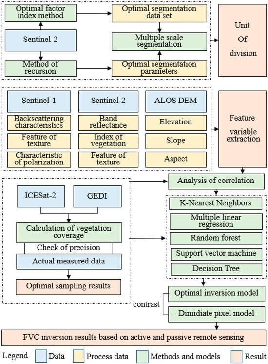
Figure 1.
Flowchart of the proposed method for FVC estimation.
3.2. Object-Oriented Segmentation
This research relies on Sentinel-2 image data and utilizes eCognition 9.0 software to perform image segmentation [33]. The best index factor method, iterative method, and evaluation tool ESP2 were applied to determine the parameters of segmentation. Additionally, the accuracy of the segmentation outcomes was assessed by comparing them with measurement data and GF-2 images, which have a spatial resolution of 0.8 m.
3.2.1. Optimal Exponential Factor Method
The optimal exponential factor method (OIF) is an effective approach for striking a balance between the information content of image bands and the information redundancy among bands [34]. The calculation formula is:
where n is the number of bands, Si is the standard deviation of band i, and Rij is the correlation coefficient between band i and band j.
3.2.2. Optimal Segmentation Parameter Evaluation
The receiver operating characteristic (ROC) curve can be used to evaluate the quality of the segmentation effect and determine the optimal segmentation scale parameters [35]. When the ROC curve presents a local peak value, the segmentation scale corresponding to the point is the optimal segmentation scale [36]. The calculation formula is:
where LV(L) is the average standard deviation of objects in the target layer L, while LV(L−1) is the average standard deviation of objects in the next layer L − 1 of the target layer L.
3.2.3. Accuracy Verification Method of Image Segmentation Results
With the use of ArcGIS 9.3, a total of 200 segmentation objects are randomly selected within the measured sample field. Subsequently, a comparison is conducted to verify the accuracy of the segmentation. If the degree of area overlap between the segmentation object and the measured data exceeds 80%, it is categorized as a correctly segmented unit.
3.3. Vegetation Cover Sampling Method for Spaceborne LiDAR
3.3.1. ICESat-2 Sampling Method for Vegetation Coverage
The spaceborne LiDAR ICESat-2 employs photon counting technology to capture three-dimensional point cloud data of terrestrial objects [37]. Through the correlation of two ICESat-2 data products, namely, the vegetation canopy height and surface elevation data (ATL03) and the surface elevation data product (ATL08), distinct categories of data are derived, including noise points, ground points, and canopy points [38]. After eliminating the noise points, a smooth spline curve method is employed to interpolate the seed points, yielding the ground profile curve. Subsequently, the relative elevation of each photon point concerning the ground is calculated, and the photon points captured by ICESat-2 within each sampling unit are tallied to compute vegetation coverage. This process facilitates the accuracy assessment of ICESat-2-based vegetation coverage concerning survey quadrat data.
Topographic Section Extraction Method
The smooth spline function curve is used to interpolate and fit the ground photon points by MATLAB 7.0 software [39]. The smooth spline algorithm is to find the optimal fitting function f(x) to minimize the penalty coefficient RSS, and the formula is as follows:
where λ is the smoothing coefficient, which is a constant and takes a value in the range 0–1. When λ = 1, f(x) can be any function that bends indefinitely through all sample points. When λ = 0, f(x) is relatively smooth and is a simple least square straight line fit.
Photon Point Classification Method
Two photon point classification methods are used in this study. The photon points were classified by using the photon point classification algorithm and the height threshold method. In this study, 10 heights were set, ranging from 0.5 m to 5.0 m, with a step size of 0.5 m [40]. Using the inversion FVC data and the measured quadrat, linear regression simulation was carried out to find the best fitting effect between the photon points of different heights and the measured data.
ICESat-2 Method for Calculating Vegetation Coverage
On the basis of photon point classification, the number of vegetation photons and ground photons was calculated [41]. The calculation formula is as follows:
where stands for vegetation coverage, stands for vegetation photon count, and stands for ground photon count.
Sampling Method of GEDI Vegetation Coverage
The spaceborne LiDAR GEDI assumes that the laser can only reach the ground by penetrating the canopy gap, ignoring the contribution of multiple reflections (<10%). Vegetation coverage is the ratio of reflected echo energy of vegetation canopy to the total reflected echo energy [42]. The formula is as follows:
where Rv is the reflected echo energy of the canopy, Rg is the reflected echo energy of the ground, and is the vegetation coverage. is the reflectance ratio between the canopy and ground, which is an empirical value.
3.4. Extraction of Feature Variables for Vegetation Coverage Modeling
3.4.1. Feature Variable Extraction Method Based on Passive Remote Sensing Data
Nearly 200 remote sensing factors related to vegetation coverage were extracted from Sentinel-1 and Sentinel-2 data. These factors encompass three variables obtained through tassel-cap transformation, three variables derived from principal component analysis, their corresponding texture characteristics (3 × 8), 10-band reflectance data, 147 spectral indices, and 2 radar vegetation indices [27,43]. The contribution degrees of these factors are analyzed, and the important factors are selected as the characteristic variables for model estimation (Table A3 and Table A4).
3.4.2. The Feature Variable Extraction Method of DEM
Topography exerts a twofold influence, impacting both the representation of vegetation in remote sensing imagery and the actual growth and distribution of plants by shaping the vegetation’s immediate environment [44]. Consequently, considering the intricate terrain characteristics in the study area, we extracted pertinent topographic factors, namely slope, slope direction, and elevation. These factors were derived from the pre-processed 10-m resolution ALOS DEM (Digital Elevation Model).
3.4.3. Feature Variable First Method
The correlation coefficient is used for correlation analysis, and the calculation formula is as follows [45]:
where n is the number of samples, xi and yi are the characteristic variables and measured vegetation coverage values in object i respectively. and is the average value of the characteristic variables of n samples and the measured vegetation coverage.
3.5. Vegetation Coverage Based on Different Algorithms
In order to find the optimal FVC modeling method, this study used stepwise multiple linear regression (DPM), support vector machine (SVM), random forest (RDF), decision tree (DT), K-Nearest Neighbors (KNN), and the random forest regression model (RDM) to establish FVC inversion models for different vegetation types [46]. The fitting ability of different regression models was compared and analyzed.
Root mean square error (RMSE) is used to measure the deviation between the measured vegetation coverage and the estimated vegetation coverage [47,48].
3.6. The Number of Samples Collected Based on Land Use and the Number of Preferred Characteristic Variables
Due to certain differences in spectral characteristics among different vegetation types, this study first classified vegetation types according to land use products, and then screened characteristic variables. The optimal feature variables of vegetation coverage modeling under different vegetation types were selected. Using the optimization method of feature variables constructed in Section 3.4, the variables were optimized according to ICESat-2 vegetation coverage quadrat points collected under different vegetation types (Table 1).

Table 1.
The number of sampling points and characteristic variables in different land use types.
4. Results
4.1. Optimal Segmentation Data Set and Factor Setting Results
Table 2 provides the standard deviations for the 10 bands of Sentinel-2 images, illustrating that the near-infrared band contains the most information, followed by visible light and short-wave infrared. In Table 3, we calculate the Pearson correlation coefficients between these 10 bands of Sentinel-2 imagery. Notably, the correlation coefficient between bands B5 and B8A, with core wavelengths of 703.9 nm and 864.8 nm, is found to be below 0.9 in comparison to the other bands. This suggests that there is limited information redundancy between these two bands and the remaining bands (Table A5). To prevent data redundancy, we systematically select one band from each set of three data sets and include the B5 and B8A band data. This process results in 18 different combinations of split data (labeled as A to R). Among these combinations, the combination F (comprising bands B2, B5, B8, B8A, and B12) exhibits the highest OIF value (522.50), signifying the most optimal segmentation effect. Consequently, this combination is employed to construct the dataset for image segmentation.
Table 2.
The standard deviation of each band of Sentinel-2 data.
Table 3.
OIF values in combinations of different Sentinel-2 bands.
In the three variables of shape, compactness, and segmentation scale, the two variables were controlled to be unchanged, and the step increment experiment was performed on one variable to determine the optimal value, the initial value of shape factor and compactness was set to 0.1, and the test was carried out with step 0.1 increments to determine the shape factor and compactness of 0.1 and 0.5, respectively. The starting value of the segmentation scale parameter was set to 10, and the step size was increased to 200 for experimentation, and the ROC-LV curve was obtained, and it was found that there were obvious “oversegmentation” and “undersegmentation” phenomena when the step size was less than 50 and greater than 150. The red line in the figure corresponds to the mutation points of local variance between 50 and 150, which can be regarded as potential optimal scale parameters. The segmentation scale is set in steps of 25, divided into four levels: 50–75, 75–100, 100–125, and 125–150, and a mutation point (59, 82, 114, 147) is selected as the optimal segmentation parameter in each level. The accuracy was verified with the field sample data, and the scale, shape, and compactness were finally selected as the best segmentation values of 82, 0.1, and 0.5, respectively, with an accuracy of 87.67% (Figure 2 and Table 4).
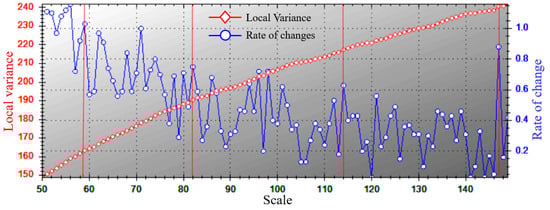
Figure 2.
ROC-LV graph based on ESP2 tools.
Table 4.
Bands description of the Sentinel-2 image.
4.2. Extraction and Evaluation of Vegetation Coverage with Spaceborne LiDAR
4.2.1. Ground Profile Extraction Results
Figure 3 shows the ground interpolation fitting curve and the distribution of the point cloud. Compared with the weak beam, more understory ground photon points can be obtained under the strong beam, and the ground terrain accuracy of interpolation fitting is higher. Therefore, in this study, only ground interpolation fitting of strong beam orbital data was performed to obtain continuous ground surface, and the ground interpolation fitting accuracy was high, and the coefficient of determination R2 was above 0.95, which met the requirements.
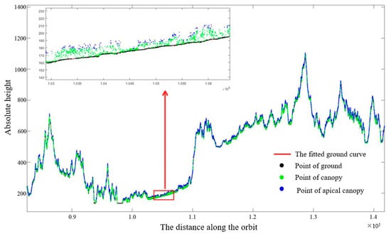
Figure 3.
Ground interpolation fitting and point cloud distribution of an intense beam.
4.2.2. ICESat-2 Sampling Accuracy of Vegetation Coverage
The accuracy analysis and verification of vegetation coverage extracted by ICESat-2 were randomly used to analyze and verify the vegetation coverage extracted by ICESat-2, and the appropriate method was chosen. It can be seen that under the separation of 0.5–2 m height threshold, the extracted vegetation coverage will be overestimated; under the separation of 2.5–3.5 m height, the extracted vegetation coverage will be overestimated at low coverage, and there is an underestimation phenomenon in high vegetation coverage, and the accuracy of vegetation coverage at different heights from largest to smallest is Cover 1.5 m > Cover 1 m > Cover 0.5 m > Cover 2 m > Cover 2.5 m > Cover ATL08 > Cover 3 m > Cover 3.5 m > Cover 4.0 m > Cover 4.5 m > Cover 5 m. In general, the accuracy of extracted vegetation coverage showed a trend of first increasing and then decreasing with the increase in separation height. The result based on the separation at a height of 1.5 m is the best. The correlation coefficient with the measured vegetation coverage is 0.853, and the R2 is 0.763 (Table 5).
Table 5.
Scatter plot of ICESat-2 and measured FVC based on different photon point classification methods.
4.2.3. Analysis of Sampling Accuracy of GEDI Vegetation Coverage
The accuracy analysis and verification of vegetation coverage extracted by GEDI were randomly used to analyze and verify the vegetation coverage extracted by GEDI, and the results showed that there was no correlation between the two, and the GEDI vegetation coverage in most of the samples was underestimated. The GEDI vegetation coverage was analyzed by using the sample square points collected by ICESat-2, which had a high correlation with the measured vegetation coverage. There are 684 identical sampling units between ICESat-2 and GEDI in the study area, and it can be seen the vegetation coverage extracted by GEDI has a positive correlation with that of ICESat-2, and the correlation is low; the size is 0.228, and the vegetation coverage of GEDI is significantly lower than that extracted from ICESat-2 (Figure 4).
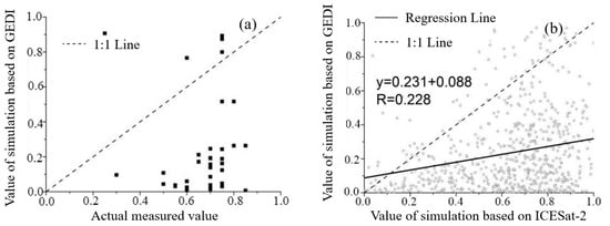
Figure 4.
Scatter plot of vegetation coverage. (a) GEDI scatter plot of vegetation coverage and measured vegetation coverage; (b) GEDI and ICESat-2 scatter plots of vegetation coverage.
4.3. Extraction and Analysis of Feature Variables of Vegetation Coverage Modeling Based on Multi-Source Data
Analyzing the relationship analysis results between 201 characteristic index variables and vegetation coverage, there was no significant correlation with vegetation coverage. The factor of 0.01 was removed, and the factors that have the strongest correlation with FVC were retained. SR65 in the vegetation index contributed the most to wetland vegetation cover modeling in different vegetation cover areas. In cropland vegetation cover modeling, band 7, SR124 and PCA1, VVEntroy and slope contributed more. In shrubland vegetation cover modeling, the contribution of multiple vegetation indices is relatively large. In the modeling of grassland vegetation cover, multiple vegetation indices contributed greatly. In broadleaf forests and others vegetation cover modeling, the vegetation index contributes the most (Figure 5).
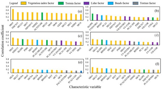
Figure 5.
Optimization results of features variables under different vegetation types. (a) Wetland, (b) Cropland, (c) Shrubland, (d) Grassland, (e) Broadleaved forest, and (f) Others.
4.4. Study on Remote Sensing Estimation of Vegetation Coverage by Comparing Multiple Algorithms
4.4.1. Analysis of Fitting Ability of Different Regression Models
Under different vegetation types, the estimation accuracy of the model established by the DPM was as follows: broadleaved forest > others > wetland > cropland > shrubland > grassland. The accuracy of the SVM for different vegetation types is: broadleaved forest > other > cropland > shrubland > grassland > wetland, all of which are less than the accuracy in the DPM model (Figure 6 and Figure 7). The accuracy of the DT for different vegetation types is: wetland > cropland > shrubland > grassland > others > broadleaved forest. The accuracy of the KNN for different vegetation types is: shrubland > grassland > others > broadleaved forest > cropland > wetland. The accuracy of the RDF is ranked as follows: broadleaved forest > others > shrubland > grassland > cropland > wetland, which is better than the evaluation accuracy of others (Table 6).
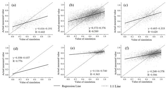
Figure 6.
Scatter diagram of FVC estimated by SVM. (a) Cropland, (b) Grassland, (c) Shrubland, (d) Wetland, (e) Broad-leaved forests, and (f) Others.
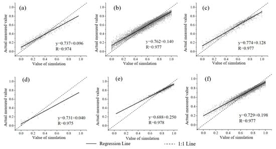
Figure 7.
FVC estimated by RDM for different (a) Cropland, (b) Grassland, (c) Shrubland, (d) Wetland, (e) Broad-leaved forest, and (f) Others.
Table 6.
Accuracy of FVC estimation model based on DPM, SVM, DT, KNN, and RDM under different vegetation types.
4.4.2. The Accuracy of the Simulation Results of Different Models
In order to fully verify the accuracy of FVC inversion of RDF constructed in this study, the accuracy of more than 1700 survey data was evaluated, and five sample set verification methods were constructed. Overall, field survey data indicate that RDF performs best among the four machine learning models. Overall, field survey data show that the RMSE of RDF is 0.026 higher than DPM. Except for Coniferous mixed forest and Relatively coniferous forest, with a tolerance of 0.05, and Shrubland and Grassland, with a tolerance of 0.15, the accuracy of other RDMs is higher than that of pixel dichotomy (Table 7 and Figure 8).
Table 7.
The accuracy of different models in simulating FVC.
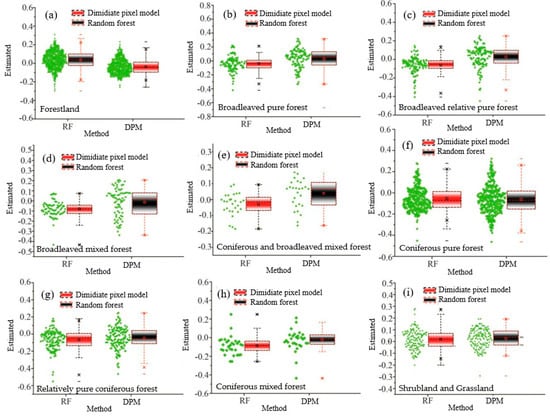
Figure 8.
Vegetation coverage error graphs of the conventional model (DPM) and the most advanced machine learning model (RDF). (a) All data, (b) Pure broadleaved forest, (c) Broadleaved relatively pure forest, (d) Mixed broadleaved forest, (e) Mixed coniferous broadleaved forest, (f) Pure coniferous forest, (g) Relatively coniferous forest, (h) CMF: Coniferous mixed forest and (i) Shrubland and grassland.
5. Discussion
5.1. Relationship Between Active and Passive Remote Sensing Feature Index and Vegetation Coverage
Due to certain differences in the spectral characteristics of different vegetation types, this study adopts the classification of vegetation types based on land use products, which is also common in other studies [49]. Subsequently, it filters characteristic variables by category and selects the optimal characteristic variables for modeling vegetation coverage across different vegetation types [50]. Specifically, considering the short growth cycle of cropland, significant variations in vegetation coverage occur from June to September. Therefore, in this study, exclusively ICESat-2 data from September was utilized for cropland sampling, ensuring synchronization with other remote sensing data. It is worth noting that similar situations have been observed in other studies; for instance, Song et al. observed relatively high time uncertainty in cropland vegetation coverage due to complex phenological variations among different crops [2]. Moreover, wetland vegetation, being relatively scarce, yielded only 33 samples, which may introduce some minor deviations into the analysis [51]. In the study area, the number of ICESat-2 laser sampling points in the taiga region is limited. Consequently, the taiga category was not separately analyzed in this study; instead, it was incorporated into other forest types for vegetation cover modeling.
5.2. Selection of Machine Learning Methods
In areas with high vegetation cover, the density of evergreen trees tends to be higher compared to the understory background vegetation, leading to more accurate estimation [52]. It is important to note that this study selected a subset of commonly used models and did not delve into deep learning methods such as CNN, FCN, and Unet [11]. The choice between these approaches depends on various factors, including the research context, the size and characteristics of the study area, and considerations regarding model operational costs, such as hardware requirements and time constraints [53]. Additionally, machine learning models can be susceptible to overfitting issues during training, and the presence of noisy data can adversely impact model training, resulting in reduced generalization performance [54]. Future research efforts should prioritize enhancing the Random Forest (RDF) model, minimizing or mitigating the covariance among different spectral indicators, and improving both accuracy and stability [55]. This will, in turn, enhance the model’s applicability for the inversion of sparse vegetation cover in the study area.
5.3. Enlightenment for Vegetation Coverage Inversion
In future studies, phenological characteristics should be fully considered to estimate vegetation cover continuously over different time changes [56]. Future studies, as well as the accuracy of FVC predictions, can also be further solved by classifying vegetation types in greater detail. The problem of spatial and temporal uncertainties may be solved by further consideration of soil, groundwater, and phenological characteristics [57]. In addition, the increase in sample size and attempts by other machine learning models are also expected to improve the inversion accuracy of vegetation coverage [58]. At present, in areas with relatively large terrain fluctuations, it may lead to a decrease in the accuracy of estimating vegetation coverage; for example, the USGS’s Landsat surface reflectance product does not consider the correction of this effect, resulting in the uncertainty of estimating vegetation cover on rugged terrain, so, in areas with complex terrain, it is recommended to use more suitable high-precision vegetation cover products [32].
6. Conclusions
The improvement in the accuracy of remote sensing extraction affecting FVC is mainly limited by the data source. Although optical remote sensing has great advantages in the extraction of vegetation coverage, due to its characteristics of orthographic projection shooting and poor penetration, signal loss from understory vegetation in dense forests will occur in dense forests, and there will be the problem that long-term series of effective data cannot be provided due to the influence of cloudy and rainy weather. By integrating data sources, this study moved beyond traditional 2D optical and radar imagery to incorporate 3D LiDAR-based vegetation analysis. The research results show that, compared with the GEDI sampling results, the threshold classification method based on ICESat-2 photon point cloud data can significantly improve the inversion accuracy of vegetation coverage. By using the RDF and combining active remote sensing data (Sentinel’s 2, 5, 8, 8A and 12 bands) and passive remote sensing data (ICESat-2 data), in the cloud coverage area, when there are serious deviations in the extraction results of the NDVI pixel binary method, the FVC can be estimated more accurately. The results of this study showed that with a single data source, it is difficult to meet the application requirements of FVC inversion evaluation. Therefore, it is necessary to combine multi-source data including radar-spectrum data to integrate and give full play to the complementary advantages of LiDAR-spectrum data.
Author Contributions
Conceptualization, Y.Y.; Software, Y.Y.; Writing—original draft, J.Y.; Writing—review & editing, Y.Y., M.S., J.Z., L.Z., L.X. and H.Z.; Visualization, Y.Y.; Project administration, Y.Y.; Funding acquisition, Y.Y. and J.L. All authors have read and agreed to the published version of the manuscript.
Funding
This research was supported by the Natural Science Foundation of Shanghai (23ZR1459700), the Youth Soft Science Research Project of Shanghai (23692120300), and the Yangfan Special Project of the Shanghai Qimingxing Program (22YF1444000).
Data Availability Statement
The original contributions presented in this study are included in the article. Further inquiries can be directed to the corresponding author.
Conflicts of Interest
The authors declare no conflicts of interest.
Appendix A
Table A1.
Remote sensing supplemental material data used in the study.
Table A1.
Remote sensing supplemental material data used in the study.
| Data Types | Description | Data Source |
|---|---|---|
| Field survey | Measurement of FVC data | Field investigation |
| Spaceborne LiDAR | ICESat-2 | https://nsidc.org/data/icesat-2, accessed on 12 January 2024 |
| GEDI | https://gedi.umd.edu/data/download, accessed on 12 January 2024 | |
| Optical remote sensing | Sentinel-2 | https://www.gscloud.cn/, accessed on 12 January 2024 |
| Synthetic aperture radar | Sentinel-1 | |
| Terrain | DEM | https://www.gscloud.cn/, accessed on 12 January 2024 |
| Land use/Land cover change | GlobeLand30 | http://www.globallandcover.com/, accessed on 12 January 2024 |
Table A2.
Land cover types, landscape metrics and other factors abbreviations.
Table A2.
Land cover types, landscape metrics and other factors abbreviations.
| Abbreviation | Description |
|---|---|
| NDVI | Normalized difference vegetation index |
| RVI | Ratio vegetation index |
| EVI | Enhanced vegetation index |
| TNDVI | Transformed normalized difference vegetation index |
| RDVI | Renormalized vegetation index |
| GEMI | Global environmental detection index |
| SAVI | Soil adjusted vegetation index |
| TSAVI | Adjustable vegetation index for transformed soil |
| CI | Red edge chlorophyll index |
| REP | Red edge position index |
| PSRI | Plant senescence reflectance index |
| NDCSI | Normalized vegetation canopy shadow index |
| NDVHVV | Normalized radar vegetation index |
| RAVHVV | Ratio radar vegetation index |
| H | Elevation |
| S | Slope |
| SinA | Sine in aspect (eastward degree) |
| CosA | Cosine in aspect (northward degree) |
Table A3.
The formula for calculating the vegetation index.
Table A3.
The formula for calculating the vegetation index.
| Vegetation Index | Calculation Formula | Number |
|---|---|---|
| NDVI | NDVI(i,j) = (bandi − bandj)/(bandi + bandj) | 45 |
| RVI | SR(i,j) = bandi/bandj | 90 |
| EVI | EVI = 2.5 × (band8 − band4)/(band8 + 6band4 − 7.5band2 + 1) | 1 |
| TNDVI | TNDVI = sqrt[(band8 − band4)/(band8 + band4) + 0.5] | 1 |
| RDVI | RDVI = (band8 − band4)/sqrt(band8 + band4) | 1 |
| GEMI | GEMI = z × (1 − 0.25 × z) − (band4 − 0.125)/(1 − band4) | 1 |
| SAVI | SAVI = 1.5 × (band8 − band4)/(band8 + band4 + 0.5) | 1 |
| TSAVI | TSAVI = 0.5 × (band8 − 0.5 × band4 − 0.5)/(0.5 × band8 + band4 − 0.15) | 1 |
| CI | CI = band7/band5 − 1 | 1 |
| REP | REP = 705 + 35 × [(band4 + band7)/2 − band5]/(band6 − band5) | 1 |
| PSRI | PSRI = (band4 − band3)/band6 | 1 |
| NDCSI | NDCSI = (band8 − band4)/(band8 + band4) × (bandi − bandimin)/(bandimax − bandimin) | 3 |
| NDVHVV | NDVHVV = (H − V)/(H + V) | 1 |
| RAVHVV | RAVHVV = V/H | 1 |
Note: bandi represents the i-th band, bandimin represents the minimum value, and bandimax represents the maximum value. H represents the backscattering intensity under horizontal polarization, while V represents the backscattering intensity under vertical polarization (V-polarization).
Table A4.
Image texture feature calculation formula and meaning.
Table A4.
Image texture feature calculation formula and meaning.
| Feature of Texture | Formula of Calculation | Meaning |
|---|---|---|
| Mean | The average gray value of remote sensing imagery reflects the uniform distribution of pixel values, and the texture regularity is positively correlated with the mean value | |
| Variance | The variance of gray value in remote sensing imagery reflects the variation degree of gray value in remote sensing image | |
| Entropy | The larger the entropy, the higher the complexity, the greater the amount of information | |
| Contrast | Reflect the clarity of remote sensing imagery | |
| Homogeneity | Reflects the magnitude of local homogeneity of remote sensing imagery | |
| Dissimilarity | The similarity degree and dissimilarity degree of texture information of remote sensing imagery are higher, which indicates that texture information has stronger uniqueness | |
| Correlation | The similarity of matrix elements in rows and columns in the gray co-occurrence matrix | |
| Angular Second Moment | Image gray distribution uniformity degree and texture thickness degree; the larger the second angular distance, the clearer the image texture, the more uniform distribution |
Note: N is the number of gray levels, is the entry (i,j) in the GLCM, and are the GLCM means, and are the GLCM variances.
Table A5.
Sentinel-2 data correlation coefficients between bands.
Table A5.
Sentinel-2 data correlation coefficients between bands.
| Correlation Coefficient | B2 | B3 | B4 | B5 | B6 | B7 | B8 | B8A | B11 | B12 |
|---|---|---|---|---|---|---|---|---|---|---|
| B2 | 1 | |||||||||
| B3 | 0.989 ** | 1 | ||||||||
| B4 | 0.967 ** | 0.983 ** | 1 | |||||||
| B5 | 0.939 ** | 0.966 ** | 0.963 ** | 1 | ||||||
| B6 | 0.727 ** | 0.767 ** | 0.706 ** | 0.824 ** | 1 | |||||
| B7 | 0.641 ** | 0.681 ** | 0.613 ** | 0.737 ** | 0.983 ** | 1 | ||||
| B8 | 0.608 ** | 0.653 ** | 0.579 ** | 0.688 ** | 0.941 ** | 0.954 ** | 1 | |||
| B8A | 0.597 ** | 0.639 ** | 0.572 ** | 0.705 ** | 0.972 ** | 0.992 ** | 0.951 ** | 1 | ||
| B11 | 0.659 ** | 0.726 ** | 0.750 ** | 0.840 ** | 0.788 ** | 0.734 ** | 0.699 ** | 0.732 ** | 1 | |
| B12 | 0.720 ** | 0.773 ** | 0.830 ** | 0.858 ** | 0.636 ** | 0.558 ** | 0.514 ** | 0.542 ** | 0.932 ** | 1 |
Note: ** represents p < 0.01.
References
- Fang, H.; Li, S.; Zhang, Y.; Wei, S.; Wang, Y. New insights of global vegetation structural properties through an analysis of canopy clumping index, fractional vegetation cover, and leaf area index. Sci. Remote Sens. 2021, 4, 100027. [Google Scholar] [CrossRef]
- Song, D.-X.; Wang, Z.; He, T.; Wang, H.; Liang, S. Estimation and validation of 30 m fractional vegetation cover over China through integrated use of Landsat 8 and Gaofen 2 data. Sci. Remote Sens. 2022, 6, 100058. [Google Scholar] [CrossRef]
- Davide, A.; Gianelle, D.; Scotton, M.; Dalponte, M. Estimating grassland vegetation cover with remote sensing: A comparison between Landsat-8, Sentinel-2 and PlanetScope imagery. Ecol. Indic. 2022, 141, 109102. [Google Scholar] [CrossRef]
- Ding, X.; Wang, Q.; Tong, X. Integrating 250 m MODIS data in spectral unmixing for 500 m fractional vegetation cover estimation. Int. J. Appl. Earth Obs. Geoinf. 2022, 111, 102860. [Google Scholar] [CrossRef]
- Wang, N.; Guo, Y.; Wei, X.; Zhou, M.; Wang, H.; Bai, Y. UAV-based remote sensing using visible and multispectral indices for the estimation of vegetation cover in an oasis of a desert. Ecol. Indic. 2022, 141, 109155. [Google Scholar] [CrossRef]
- Zhu, C.; Tian, J.; Tian, Q.; Wang, X.; Li, Q. Using NDVI-NSSI feature space for simultaneous estimation of fractional cover of non-photosynthetic vegetation and photosynthetic vegetation. Int. J. Appl. Earth Obs. Geoinf. 2023, 118, 103282. [Google Scholar] [CrossRef]
- Younes, N.; Joyce, K.E.; Northfield, T.D.; Maier, S.W. The effects of water depth on estimating Fractional Vegetation Cover in mangrove forests. Int. J. Appl. Earth Obs. Geoinf. 2019, 83, 101924. [Google Scholar] [CrossRef]
- Liu, J.; Fan, J.; Yang, C.; Xu, F.; Zhang, X. Novel vegetation indices for estimating photosynthetic and non-photosynthetic fractional vegetation cover from Sentinel data. Int. J. Appl. Earth Obs. Geoinf. 2022, 109, 102793. [Google Scholar] [CrossRef]
- Gao, L.; Wang, X.; Johnson, B.A.; Tian, Q.; Wang, Y.; Verrelst, J.; Mu, X.; Gu, X. Remote sensing algorithms for estimation of fractional vegetation cover using pure vegetation index values: A review. ISPRS J. Photogramm. Remote Sens. 2020, 159, 364–377. [Google Scholar] [CrossRef] [PubMed]
- Tian, J.; Zhang, Z.; Philpot, W.D.; Tian, Q.; Zhan, W.; Xi, Y.; Wang, X.; Zhu, C. Simultaneous estimation of fractional cover of photosynthetic and non-photosynthetic vegetation using visible-near infrared satellite imagery. Remote Sens. Environ. 2023, 290, 113549. [Google Scholar] [CrossRef]
- Chen, D.; Zhang, F.; Zhang, M.; Meng, Q.; Jim, C.Y.; Shi, J.; Tan, M.L.; Ma, X. Landscape and vegetation traits of urban green space can predict local surface temperature. Sci. Total Environ. 2022, 825, 154006. [Google Scholar] [CrossRef] [PubMed]
- Verrelst, J.; Halabuk, A.; Atzberger, C.; Hank, T.; Steinhauser, S.; Berger, K. A comprehensive survey on quantifying non-photosynthetic vegetation cover and biomass from imaging spectroscopy. Ecol. Indic. 2023, 155, 110911. [Google Scholar] [CrossRef]
- Zhou, Y.; Lao, C.; Yang, Y.; Zhang, Z.; Chen, H.; Chen, Y.; Chen, J.; Ning, J.; Yang, N. Diagnosis of winter-wheat water stress based on UAV-borne multispectral image texture and vegetation indices. Agric. Water Manag. 2021, 256, 107076. [Google Scholar] [CrossRef]
- Dou, Y.; Tian, F.; Wigneron, J.-P.; Tagesson, T.; Du, J.; Brandt, M.; Liu, Y.; Zou, L.; Kimball, J.S.; Fensholt, R. Reliability of using vegetation optical depth for estimating decadal and interannual carbon dynamics. Remote Sens. Environ. 2023, 285, 113390. [Google Scholar] [CrossRef]
- Sinha, S.K.; Padalia, H.; Dasgupta, A.; Verrelst, J.; Rivera, J.P. Estimation of leaf area index using PROSAIL based LUT inversion, MLRA-GPR and empirical models: Case study of tropical deciduous forest plantation, North India. Int. J. Appl. Earth Obs. Geoinf. 2020, 86, 102027. [Google Scholar] [CrossRef] [PubMed]
- Mao, P.; Zhang, J.; Li, M.; Liu, Y.; Wang, X.; Yan, R.; Shen, B.; Zhang, X.; Shen, J.; Zhu, X.; et al. Spatial and temporal variations in fractional vegetation cover and its driving factors in the Hulun Lake region. Ecol. Indic. 2022, 135, 108490. [Google Scholar] [CrossRef]
- Li, X.; Wigneron, J.-P.; Frappart, F.; Lannoy, G.D.; Fan, L.; Zhao, T.; Gao, L.; Tao, S.; Ma, H.; Peng, Z.; et al. The first global soil moisture and vegetation optical depth product retrieved from fused SMOS and SMAP L-band observations. Remote Sens. Environ. 2022, 282, 113272. [Google Scholar] [CrossRef]
- Li, L.; Mu, X.; Jiang, H.; Chianucci, F.; Hu, R.; Song, W.; Qi, J.; Liu, S.; Zhou, J.; Chen, L.; et al. Review of ground and aerial methods for vegetation cover fraction (fCover) and related quantities estimation: Definitions, advances, challenges, and future perspectives. ISPRS J. Photogramm. Remote Sens. 2023, 199, 133–156. [Google Scholar] [CrossRef]
- Zhang, J.; Zhang, Y.; Zhou, T.; Sun, Y.; Yang, Z.; Zheng, S. Research on the identification of land types and tree species in the Engebei ecological demonstration area based on GF-1 remote sensing. Ecol. Inform. 2023, 77, 102242. [Google Scholar] [CrossRef]
- Mousivand, A.; Menenti, M.; Gorte, B.; Verhoef, W. Multi-temporal, multi-sensor retrieval of terrestrial vegetation properties from spectral–directional radiometric data. Remote Sens. Environ. 2015, 158, 311–330. [Google Scholar] [CrossRef]
- Hu, L.; Zhao, T.; Ju, W.; Peng, Z.; Shi, J.; Rodríguez-Fernández, N.J.; Wigneron, J.-P.; Cosh, M.H.; Yang, K.; Lu, H.; et al. A twenty-year dataset of soil moisture and vegetation optical depth from AMSR-E/2 measurements using the multi-channel collaborative algorithm. Remote Sens. Environ. 2023, 292, 113595. [Google Scholar] [CrossRef]
- Yan, X.; Zuo, C.; Li, Z.; Chen, H.W.; Jiang, Y.; He, B.; Liu, H.; Chen, J.; Shi, W. Cooperative simultaneous inversion of satellite-based real-time PM2.5 and ozone levels using an improved deep learning model with attention mechanism. Environ. Pollut. 2023, 327, 121509. [Google Scholar] [CrossRef] [PubMed]
- Yang, Y.; Guangrong, S.; Chen, Z.; Hao, S.; Zhouyiling, Z.; Shan, Y. Quantitative analysis and prediction of urban heat island intensity on urban–rural gradient: A case study of Shanghai. Sci. Total. Environ. 2022, 829, 154264. [Google Scholar] [CrossRef] [PubMed]
- Nill, L.; Grünberg, I.; Ullmann, T.; Gessner, M.; Boike, J.; Hostert, P. Arctic shrub expansion revealed by Landsat-derived multitemporal vegetation cover fractions in the Western Canadian Arctic. Remote Sens. Environ. 2022, 281, 113228. [Google Scholar] [CrossRef]
- Che, L.; Zhang, H.; Wan, L. Spatial distribution of permafrost degradation and its impact on vegetation phenology from 2000 to 2020. Sci. Total Environ. 2023, 877, 162889. [Google Scholar] [CrossRef] [PubMed]
- Schiefer, F.; Schmidtlein, S.; Kattenborn, T. The retrieval of plant functional traits from canopy spectra through RTM-inversions and statistical models are both critically affected by plant phenology. Ecol. Indic. 2021, 121, 107062. [Google Scholar] [CrossRef]
- Zhang, N.; Li, Z.; Feng, Y.; Li, X.; Tang, J. Development and application of a vegetation degradation classification approach for the temperate grasslands of northern China. Ecol. Indic. 2023, 154, 110857. [Google Scholar] [CrossRef]
- Ciccioli, P.; Silibello, C.; Finardi, S.; Pepe, N.; Ciccioli, P.; Rapparini, F.; Neri, L.; Fares, S.; Brilli, F.; Mircea, M.; et al. The potential impact of biogenic volatile organic compounds (BVOCs) from terrestrial vegetation on a Mediterranean area using two different emission models. Agric. For. Meteorol. 2023, 328, 109255. [Google Scholar] [CrossRef]
- Yang, S.; Yang, J.; Shi, S.; Song, S.; Luo, Y.; Du, L. The rising impact of urbanization-caused CO2 emissions on terrestrial vegetation. Ecol. Indic. 2023, 148, 110079. [Google Scholar] [CrossRef]
- Tian, J.; Liu, J.; Wang, J.; Li, C.; Yu, F.; Chu, Z. A spatio-temporal evaluation of the WRF physical parameterisations for numerical rainfall simulation in semi-humid and semi-arid catchments of Northern China. Atmos. Res. 2017, 191, 141–155. [Google Scholar] [CrossRef]
- Guo, H.; Shi, M.; Yang, J.; Chen, C. Precise spatial distribution of suitability of Pinus tabulaeformis in Daqing River Basin, Baiyangdian. J. Zhejiang AF Univ. 2021, 38, 1100–1108. (In Chinese) [Google Scholar] [CrossRef]
- Guo, Z.; Wang, T.; Liu, S.; Kang, W.; Chen, X.; Feng, K.; Zhi, Y. Comparison of the backpropagation network and the random forest algorithm based on sampling distribution effects consideration for estimating nonphotosynthetic vegetation cover. Int. J. Appl. Earth Obs. Geoinf. 2021, 104, 102573. [Google Scholar] [CrossRef]
- Yi, Y.; Shi, M.; Gao, M.; Zhang, G.; Xing, L.; Zhang, C.; Xie, J. Comparative Study on Object-Oriented Identification Methods of Plastic Greenhouses Based on Landsat Operational Land Imager. Land 2023, 12, 121120. [Google Scholar] [CrossRef]
- Chavez, P.S.; Berlin, G.L.; Sowers, L.B. Statistical method for selecting Landsat MSS ratios. J. Appl. Photogr. Eng. 1982, 8, 23–30. [Google Scholar]
- Liang, L.; Li, X.; Huang, Y.; Qin, Y.; Huang, H. Integrating remote sensing, GIS and dynamic models for landscape-level simulation of forest insect disturbance. Ecol. Model. 2017, 354, 1–10. [Google Scholar] [CrossRef]
- Liu, G.; Jin, Q.; Li, J.; Li, L.; He, C.; Huang, Y.; Yao, Y. Policy factors impact analysis based on remote sensing data and the CLUE-S model in the Lijiang River Basin, China. Catena 2017, 158, 286–297. [Google Scholar] [CrossRef]
- Zhao, R.; Ni, W.; Zhang, Z.; Dai, H.; Yang, C.; Li, Z.; Liang, Y.; Liu, Q.; Pang, Y.; Li, Z.; et al. Optimizing ground photons for canopy height extraction from ICESat-2 data in mountainous dense forests. Remote Sens. Environ. 2023, 299, 113851. [Google Scholar] [CrossRef]
- Zang, J.; Ni, W.; Zhang, Y. Spatially-explicit mapping annual oil palm heights in peninsular Malaysia combining ICESat-2 and stand age data. Remote Sens. Environ. 2023, 295, 113693. [Google Scholar] [CrossRef]
- Chen, C.; Wu, H.; Yang, Z.; Li, Y. Adaptive coarse-to-fine clustering and terrain feature-aware-based method for reducing LiDAR terrain point clouds. ISPRS J. Photogramm. Remote Sens. 2023, 200, 89–105. [Google Scholar] [CrossRef]
- Neuenschwander, A.; Pitts, K. The ATL08 land and vegetation product for the ICESat-2 Mission. Remote Sens. Environ. 2019, 221, 247–259. [Google Scholar] [CrossRef]
- Narine, L.L.; Popescu, S.; Neuenschwander, A.; Zhou, T.; Srinivasan, S.; Harbeck, K. Estimating aboveground biomass and forest canopy cover with simulated ICESat-2 data. Remote Sens. Environ. 2019, 224, 1–11. [Google Scholar] [CrossRef]
- Ni-Meister, W.; Jupp, D.L.B.; Dubayah, R. Modeling LiDAR Waveforms in Heterogeneous and Discrete Canopies. IEEE Trans. Geosci. Remote Sens. 2001, 39, 1943–1958. [Google Scholar] [CrossRef]
- Tillack, A.; Clasen, A.; Kleinschmit, B.; Förster, M. Estimation of the seasonal leaf area index in an alluvial forest using high-resolution satellite-based vegetation indices. Remote Sens. Environ. 2014, 141, 52–63. [Google Scholar] [CrossRef]
- Fan, J.; Xu, Y.; Ge, H.; Yang, W. Vegetation growth variation in relation to topography in Horqin Sandy Land. Ecol. Indic. 2020, 113, 106215. [Google Scholar] [CrossRef]
- Yi, Y.; Shi, M.; Yi, X.D.; Liu, J.L.; Shen, G.R.; Yang, N.; Hu, X.L. Dynamic Changes of Plantations and Natural Forests in the Middle Reaches of the Yangtze River and Their Relationship with Climatic Factors. Forests 2022, 13, 1224. [Google Scholar] [CrossRef]
- Purwanto Latifah, S.; Yonariza Akhsani, F.; Sofiana, E.I.; Ferdiansah, M.R. Land cover change assessment using random forest and CA markov from remote sensing images in the protected forest of South Malang, Indonesia. Remote Sens. Appl. Soc. Environ. 2023, 32, 101061. [Google Scholar] [CrossRef]
- Ćalasan, M.; Abdel Aleem, S.H.E.; Zobaa, A.F. On the root mean square error (RMSE) calculation for parameter estimation of photovoltaic models: A novel exact analytical solution based on Lambert W function. Energy Convers. Manag. 2020, 210, 112716. [Google Scholar] [CrossRef]
- Zhu, W.; Yu, X.; Wei, J.; Lv, A. Surface flux equilibrium estimates of evaporative fraction and evapotranspiration at global scale: Accuracy evaluation and performance comparison. Agric. Water Manag. 2024, 291, 108609. [Google Scholar] [CrossRef]
- Sun, L.; Zhao, D.; Zhang, G.; Wu, X.; Yang, Y.; Wang, Z. Using SPOT VEGETATION for analyzing dynamic changes and influencing factors on vegetation restoration in the Three-River Headwaters Region in the last 20 years (2000–2019), China. Ecol. Eng. 2022, 183, 106742. [Google Scholar] [CrossRef]
- Wu, S.; Yang, P.; Ren, J.; Chen, Z.; Liu, C.; Li, H. Winter wheat LAI inversion considering morphological characteristics at different growth stages coupled with microwave scattering model and canopy simulation model. Remote Sens. Environ. 2020, 240, 111681. [Google Scholar] [CrossRef]
- Yue, J.; Tian, Q.; Dong, X.; Xu, N. Using broadband crop residue angle index to estimate the fractional cover of vegetation, crop residue, and bare soil in cropland systems. Remote Sens. Environ. 2020, 237, 111538. [Google Scholar] [CrossRef]
- Wang, B.; Jia, K.; Wei, X.; Xia, M.; Yao, Y.; Zhang, X.; Liu, D.; Tao, G. Generating spatiotemporally consistent fractional vegetation cover at different scales using spatiotemporal fusion and multiresolution tree methods. ISPRS J. Photogramm. Remote Sens. 2020, 167, 214–229. [Google Scholar] [CrossRef]
- Deng, Y.; Wang, X.; Wang, K.; Ciais, P.; Tang, S.; Jin, L.; Li, L.; Piao, S. Responses of vegetation greenness and carbon cycle to extreme droughts in China. Agric. For. Meteorol. 2021, 298, 108307. [Google Scholar] [CrossRef]
- Hong, P.; Xiao, J.; Liu, H.; Niu, Z.; Ma, Y.; Wang, Q.; Zhang, D.; Ma, Y. An inversion model of microplastics abundance based on satellite remote sensing: A case study in the Bohai Sea. Sci. Total Environ. 2024, 909, 168537. [Google Scholar] [CrossRef] [PubMed]
- Ali, E.; Xu, W.; Ding, X. Improved optical image matching time series inversion approach for monitoring dune migration in North Sinai Sand Sea: Algorithm procedure, application, and validation. ISPRS J. Photogramm. Remote Sens. 2020, 164, 106–124. [Google Scholar] [CrossRef]
- Bai, X.; Zhao, W.; Ji, S.; Qiao, R.; Dong, C.; Chang, X. Estimating fractional cover of non-photosynthetic vegetation for various grasslands based on CAI and DFI. Ecol. Indic. 2021, 131, 108252. [Google Scholar] [CrossRef]
- Jia, K.; Liang, S.; Gu, X.; Baret, F.; Wei, X.; Wang, X.; Yao, Y.; Yang, L.; Li, Y. Fractional vegetation cover estimation algorithm for Chinese GF-1 wide field view data. Remote Sens. Environ. 2016, 177, 184–191. [Google Scholar] [CrossRef]
- Vermeulen, L.M.; Munch, Z.; Palmer, A. Fractional vegetation cover estimation in southern African rangelands using spectral mixture analysis and Google Earth Engine. Comput. Electron. Agric. 2021, 182, 105980. [Google Scholar] [CrossRef]
Disclaimer/Publisher’s Note: The statements, opinions and data contained in all publications are solely those of the individual author(s) and contributor(s) and not of MDPI and/or the editor(s). MDPI and/or the editor(s) disclaim responsibility for any injury to people or property resulting from any ideas, methods, instructions or products referred to in the content. |
© 2025 by the authors. Licensee MDPI, Basel, Switzerland. This article is an open access article distributed under the terms and conditions of the Creative Commons Attribution (CC BY) license (https://creativecommons.org/licenses/by/4.0/).