
Applicability of Visible–Near-Infrared Spectroscopy to Predicting Water Retention in Japanese Forest Soils


Abstract
1. Introduction
2. Materials and Methods
2.1. Study Area
2.2. Soil Samples
2.3. Spectroscopic Analysis
2.4. EBM
2.5. Performance Evaluation
3. Results
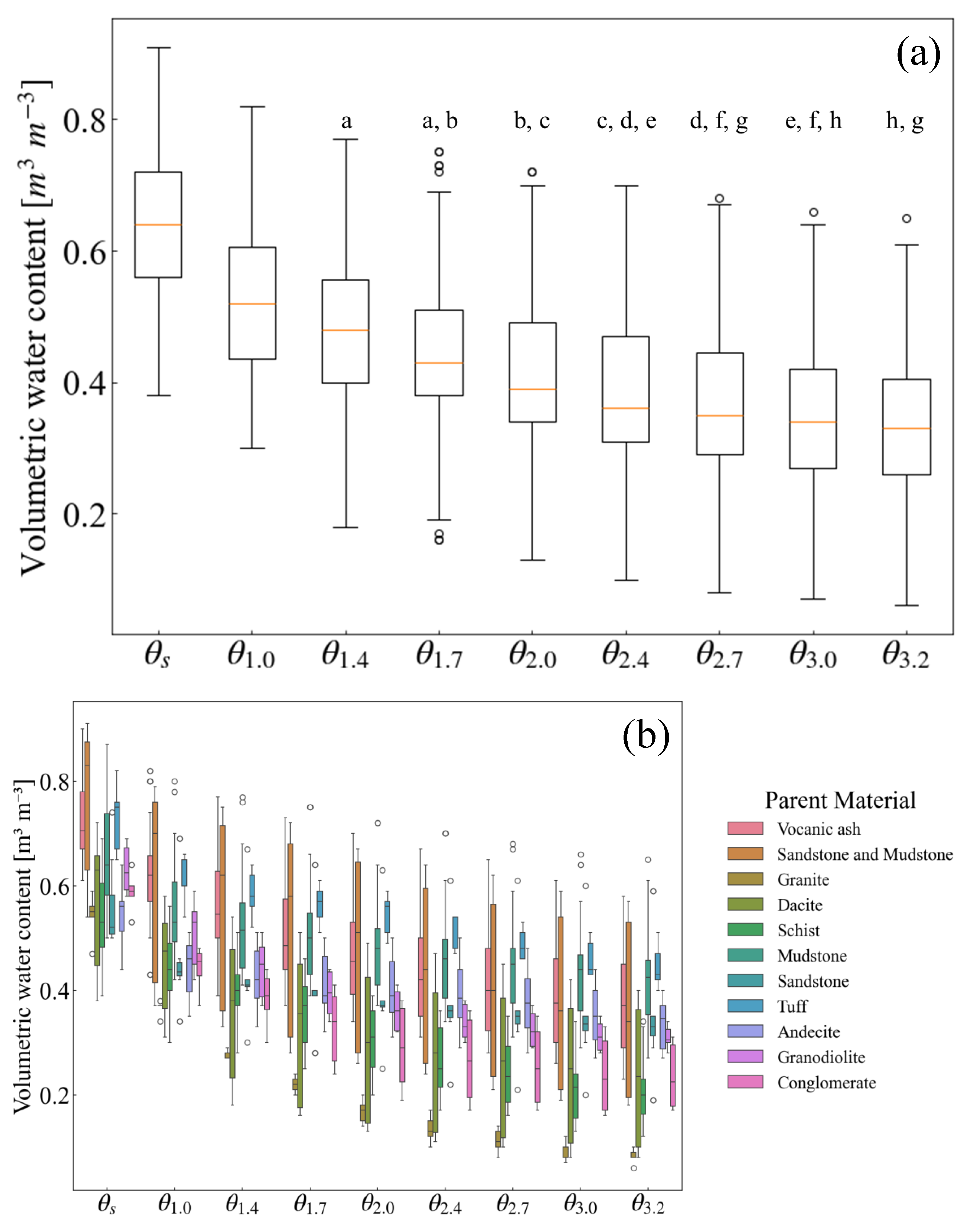
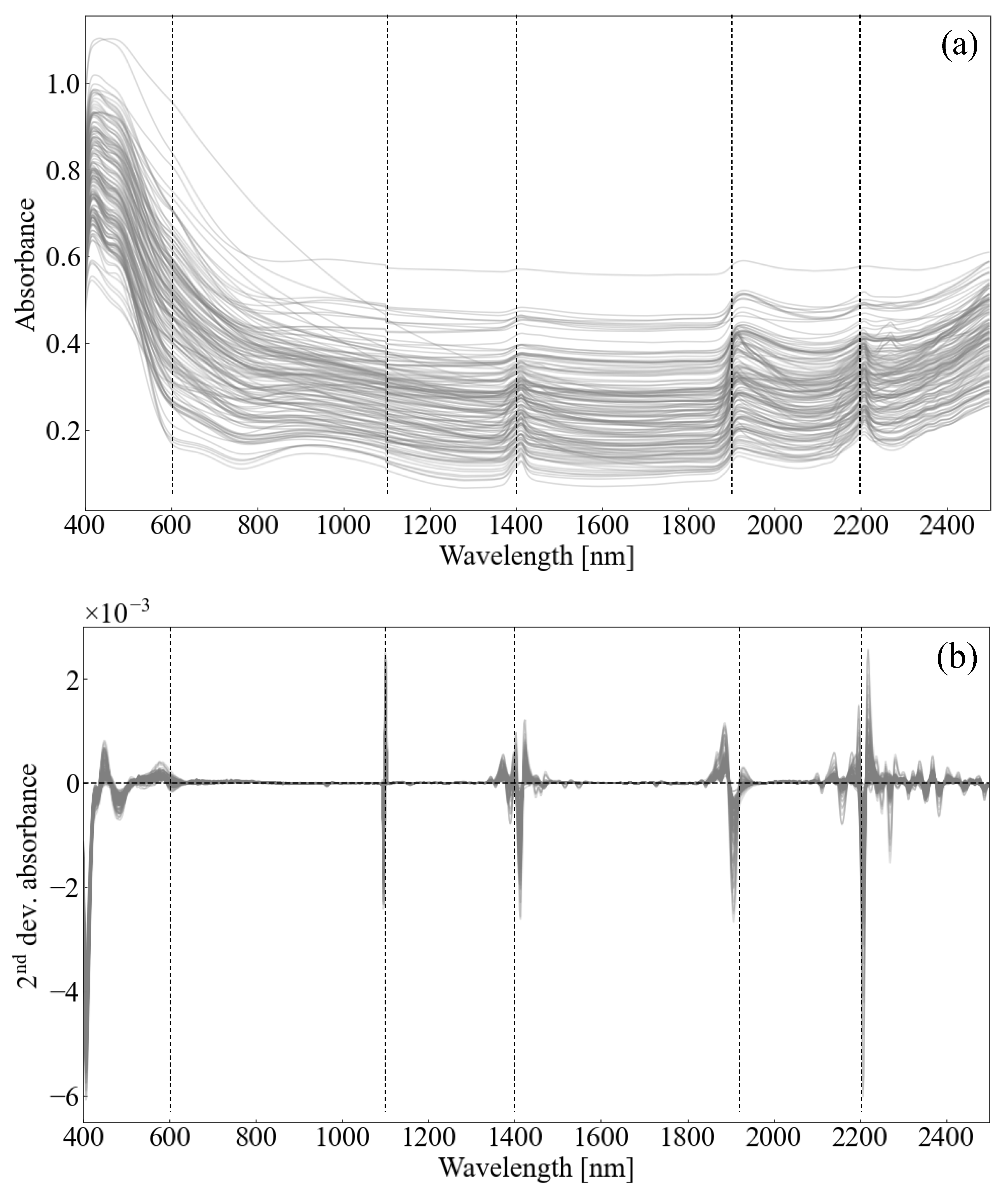
3.1. Measurements
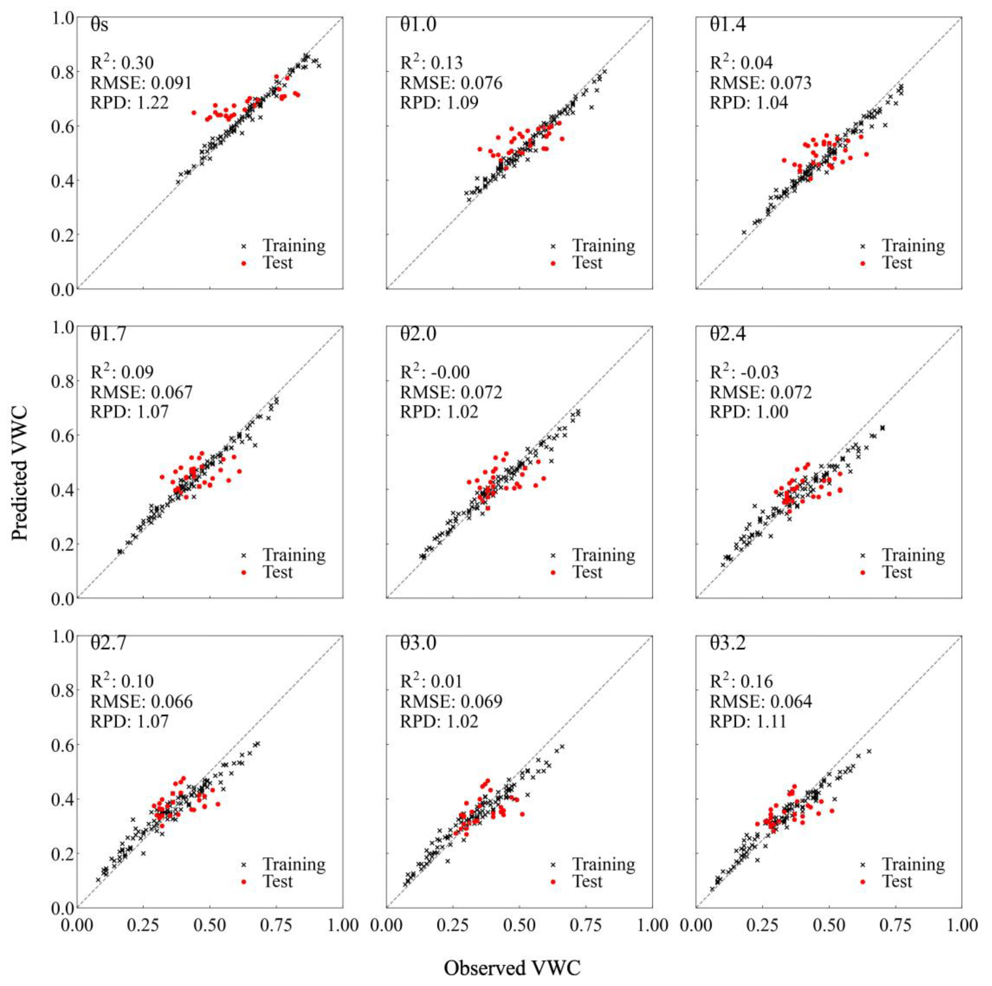
3.2. Prediction Performance
4. Discussion
5. Conclusions
Author Contributions
Funding
Data Availability Statement
Conflicts of Interest
Abbreviations
| EBM | Explainable boosting machine |
| LIME | Local interpretable model-agnostic explanations |
| PLS | Partial least-squares |
| RMSE | Root mean squared error |
| RPD | Ratio of performance to deviation |
| SHAP | Shapley additive explanations |
| SOC | Soil organic carbon |
| Vis-NIR | Visible-Near-Infrared spectroscopy |
| WRB | World Reference Base for Soil Resources |
References
- IPCC. Summary for Policymakers. In Climate Change 2023: Synthesis Report. Contribution of Working Groups I, II, and III to the Sixth Assessment Report of the Intergovernmental Panel on Climate Change; Core Writing Team, Lee, H., Romero, J., Eds.; IPCC: Geneva, Switzerland, 2023; pp. 1–34. Available online: https://www.ipcc.ch/report/ar6/syr/downloads/report/IPCC_AR6_SYR_SPM.pdf (accessed on 5 July 2025).
- Shepherd, K.D.; Walsh, M.G. Infrared spectroscopy—Enabling an evidence-based diagnostic surveillance approach to agricultural and environmental management in developing countries. J. Near Infrared Spec. 2007, 15, 1–19. [Google Scholar] [CrossRef]
- Stenberg, B.; Viscarra Rossel, R.A.; Mouazen, A.M.; Wetterlind, J. Chapter five—Visible and near infrared spectroscopy in soil science. Adv. Agron. 2010, 107, 163–215. [Google Scholar] [CrossRef]
- Mohamed, E.S.; Saleh, A.M.; Belal, A.B.; Gad, A. Application of near-infrared reflectance for quantitative assessment of soil properties. Egypt. J. Remote Sens. Space Sci. 2018, 21, 1–14. [Google Scholar] [CrossRef]
- Janik, L.J.; Merry, R.H.; Skjemstad, J.O. Can mid infrared diffuse reflectance analysis replace soil extractions? Aust. J. Exp. Agric. 1998, 38, 681–696. [Google Scholar] [CrossRef]
- Minasny, B.; McBratney, A.B.; Tranter, G.; Murphy, B.W. Using soil knowledge for the evaluation of mid-infrared diffuse reflectance spectroscopy for predicting soil physical and mechanical properties. Eur. J. Soil. Sci. 2008, 59, 960–971. [Google Scholar] [CrossRef]
- Vestergaard, R.-J.; Vasava, H.B.; Aspinall, D.; Chen, S.; Gillespie, A.; Adamchuk, V.; Biswas, A. Evaluation of optimized preprocessing and modeling algorithms for prediction of soil properties using VIS–NIR spectroscopy. Sensors 2021, 21, 6745. [Google Scholar] [CrossRef] [PubMed]
- Norouzi, S.; Sadeghi, M.; Tuller, M.; Ebrahimian, H.; Liaghat, A.; Jones, S.B. A novel laboratory method for the retrieval of the soil water retention curve from shortwave infrared reflectance. J. Hydrol. 2023, 626, 130284. [Google Scholar] [CrossRef]
- Fouad, Y.; Soltani, I.; Cudennec, C.; Michot, D. Using near-infrared spectroscopy to estimate soil water retention curves with the van Genuchten model. Geoderma 2025, 454, 117175. [Google Scholar] [CrossRef]
- De Melo, T.M.; Pedrollo, O.C. Artificial neural networks for estimating soil water retention curve using fitted and measured data. Appl. Environ. Soil. Sci. 2015, 2015, 535216. [Google Scholar] [CrossRef]
- Rossel, R.A.V.; Behrens, T. Using data mining to model and interpret soil diffuse reflectance spectra. Geoderma 2010, 158, 46–54. [Google Scholar] [CrossRef]
- Wadoux, A.M.J.-C. Interpretable spectroscopic modelling of soil with machine learning. Eur. J. Soil. Sci. 2023, 74, e13370. [Google Scholar] [CrossRef]
- Lundberg, S.M.; Lee, S.I. A Unified approach to interpreting model predictions. In Proceedings of the 2017 Conference on Neural Information Processing Systems, Long Beach, CA, USA, 4–9 December 2017; Volume 30. [Google Scholar]
- Ribeiro, M.T.; Singh, S.; Guestrin, C. “Why should I trust you?”: Explaining the predictions of any classifier. In Proceedings of the 22nd ACM SIGKDD International Conference on Knowledge Discovery and Data Mining, San Francisco, CA, USA, 13–17 August 2016; IEEE: San Francisco, CA, USA, 2016; pp. 1135–1144. [Google Scholar]
- Rudin, C. Stop explaining black box machine learning models for high stakes decisions and use interpretable models instead. Nat. Mach. Intell. 2019, 1, 206–215. [Google Scholar] [CrossRef] [PubMed]
- Molnar, C. Interpretable Machine Learning: A Guide for Making Black Box Models Explainable. 2022. Available online: https://christophm.github.io/interpretable-ml-book/ (accessed on 5 July 2025).
- Caruana, R.; Lou, Y.; Gehrke, J.; Koch, P.; Sturm, M.; Elhadad, N. Intelligible models for healthcare: Predicting pneumonia risk and hospital 30-day readmission. In Proceedings of the 21st ACM SIGKDD International Conference on Knowledge Discovery and Data Mining (KDD ‘15), Sydney, Australia, 10–13 August 2015; Association for Computing Machinery: New York, NY, USA, 2015; pp. 1721–1730. [Google Scholar]
- Lou, Y.; Caruana, R.; Gehrke, J.; Hooker, G. Accurate intelligible models with pairwise interactions. In Proceedings of the 19th ACM SIGKDD International Conference on Knowledge Discovery and Data Mining, Chicago, IL, USA, 11–14 August 2013; ACM: New York, NY, USA, 2013; pp. 623–631. [Google Scholar]
- Microsoft InterpretML Project. InterpretML: A Unified Framework for Machine Learning Interpretability. Available online: https://interpret.ml/docs/ebm.html (accessed on 3 July 2025).
- Blaschek, M.; Roudier, P.; Poggio, M.; Hedley, C.B. Prediction of soil available water-holding capacity from visible near-infrared reflectance spectra. Sci. Rep. 2019, 9, 12833. [Google Scholar] [CrossRef] [PubMed]
- Baumann, P.; Lee, J.; Behrens, T.; Biswas, A.; Six, J.; McLachlan, G.; Viscarra Rossel, R.A. Modelling soil water retention and water-holding capacity with visible–near-infrared spectra and machine learning. Eur. J. Soil Sci. 2022, 73, 13220. [Google Scholar] [CrossRef]
- Conforti, M.; Castrignanò, A.; Robustelli, G.; Scarciglia, F.; Stelluti, M.; Buttafuoco, G. Laboratory-based Vis–NIR spectroscopy and partial least square regression with spatially correlated errors for predicting spatial variation of soil organic matter content. CATENA 2015, 124, 60–67. [Google Scholar] [CrossRef]
- Nanko, K.; Ugawa, S.; Hashimoto, S.; Imaya, A.; Kobayashi, M.; Sakai, H.; Ishizuka, S.; Miura, S.; Tanaka, N.; Takahashi, M. A Pedotransfer function for estimating bulk density of forest soil in japan affected by volcanic ash. Geoderma 2014, 213, 36–45. [Google Scholar] [CrossRef]
- Chinilin, A.V.; Vindeker, G.V.; Savin, I.Y. Vis-NIR Spectroscopy for Soil Organic Carbon Assessment: A Meta-Analysis. Eurasian Soil Sc. 2023, 56, 1605–1617. [Google Scholar] [CrossRef]
- Liu, S.; Shen, H.; Chen, S.; Zhao, X.; Biswas, A.; Jia, X.; Shi, Z.; Fang, J. Estimating forest soil organic carbon content using vis-nir spectroscopy: Implications for large-scale soil carbon spectroscopic assessment. Geoderma 2019, 348, 37–44. [Google Scholar] [CrossRef]
- Soil Classification System of Japan. The Fifth Committee for Soil Classification and Nomenclature of Japanese Society of Pedology; The Japanese Society of Pedology: Sendai, Japan, 2017. (In Japanese) [Google Scholar]
- IUSS Working Group WRB. World Reference Base for Soil Resources: International Soil Classification System for Naming Soils and Creating Legends for Soil Maps, 4th ed.; International Union of Soil Sciences: Vienna, Austria, 2022. [Google Scholar]
- Imaya, A.; Noguchi, A.; Watanabe, A.; Ito, C.; Takakai, F.; Shinmachi, F.; Uno, F.; Fujisawa, H.; Miura, H.; Kubotera, H.; et al. The Soils of, Japan; Hatano, R., Shinjo, H., Takata, Y., Eds.; Springer: Singapore, 2021. [Google Scholar]
- Savitzky, A.; Golay, M.J.E. Smoothing and differentiation of data by simplified least squares procedures. Anal. Chem. 1964, 36, 1627–1639. [Google Scholar] [CrossRef]
- Riley, R.D.; Snell, K.I.E.; Ensor, J.; Burke, D.L.; Harrell, F.E.; Moons, K.G.M.; Collins, G.S. Minimum sample size for developing a multivariable prediction model: Part I—Continuous outcomes. Stat. Med. 2019, 38, 1262–1275. [Google Scholar] [CrossRef] [PubMed]
- Python Software Foundation Python Language Reference, Version 3.12.3. 2024. Available online: https://www.python.org (accessed on 5 July 2025).
- Pedregosa, F.; Varoquaux, G.; Gramfort, A.; Michel, V.; Bertrand, T.; Grisel, O. Machine Learning in Python. J. Mach. Learn. Res. 2011, 12, 2825–2830. [Google Scholar]
- Core Team. R: A Language and Environment for Statistical Computing, Version 4.4.0. R Foundation for Statistical Computing. 2024. Available online: https://www.R-project.org/ (accessed on 5 July 2025).
- Hothorn, T.; Bretz, F.; Westfall, P. Simultaneous inference in general parametric models. Biom. J. 2008, 50, 346–363. [Google Scholar] [CrossRef] [PubMed]
- McGuirk, H.A.; Cairns, A. Relationships between Soil Moisture and Visible–NIR Soil Reflectance: A Review Presenting New Analyses and Data to Fill the Gaps. Geotechnics 2024, 4, 78–108. [Google Scholar] [CrossRef]
- Weyer, L.G.; Lo, S.-C. Spectra—structure correlations in the near-infrared. In Handbook of Vibrational Spectroscopy; Chalmers, J.M., Griffiths, P.R., Eds.; Wiley: New York, NY, USA, 2006; pp. 1817–1837. [Google Scholar]
- Pittaki-Chrysodonta, Z.; Moldrup, P.; Knadel, M.; Iversen, B.V.; Hermansen, C.; Greve, M.H.; de Jonge, L.W. Predicting the campbell soil water retention function: Comparing visible–near-infrared spectroscopy with classical pedotransfer function. Vadose Zone J. 2018, 17, 1–12. [Google Scholar] [CrossRef]
- Ben-Dor, E. The reflectance spectra of organic matter in the visible near-infrared and short wave infrared region (400–2500 Nm) during a controlled decomposition process. Remote Sens. Environ. 1997, 61, 1–15. [Google Scholar] [CrossRef]
- Demattê, J.A.M.; Campos, R.C.; Alves, M.C.; Fiorio, P.R.; Nanni, M.R. Visible–NIR reflectance: A new approach on soil evaluation. Geoderma 2004, 121, 95–112. [Google Scholar] [CrossRef]
- Viscarra Rossel, R.A.; McBratney, A.B. Laboratory evaluation of a proximal sensing technique for simultaneous measurement of soil clay and water content. Geoderma 1998, 85, 19–39. [Google Scholar] [CrossRef]
- Roth, K.; Sanderson, M.; Koestel, J.; Jarvis, N. Rapid estimation of soil water retention curves using visible–near infrared spectroscopy. J. Hydrol. 2021, 603, 127195. [Google Scholar] [CrossRef]
- Lalitha, M.; Sarkar, D.; Bhowmik, A.; Chakraborty, S.; Das, T.; Kundu, D. Field-scale prediction of soil moisture retention parameters using VNIR–SWIR spectroscopy and machine learning. Geoderma 2022, 417, 115816. [Google Scholar]
- Oberholzer, S.; Summerauer, L.; Steffens, M.; Ifejika Speranza, C. Best performances of visible–near-infrared models in soils with little carbonate—A field study in Switzerland. Soil 2024, 10, 231–249. [Google Scholar] [CrossRef]
- Jeong, S.; Kim, Y.-K.; Hur, S.H.; Bang, H.; Kim, H.; Chung, H. Explainable extreme gradient boosting as a machine learning tool for discrimination of the geographical origin of chili peppers using laser ablation-inductively coupled plasma mass spectrometry, X-ray fluorescence, and near-infrared spectroscopy. J. Agric. Food Res. 2024, 18, 101446. [Google Scholar] [CrossRef]


| Sampling Number | Latitude (N) Longitude (E) | Horizon | Sampling Depth [cm] | Parent Material | Sample Volume [cm3] | Bulk Density [g cm−3] |
|---|---|---|---|---|---|---|
| 1 | 36.1845 140.218 | A1 | 10 | Volcanic ash | 400 | 0.89 |
| A2 | 30 | 400 | 0.83 | |||
| B1 | 54 | 400 | 0.70 | |||
| B2 | 85 | 400 | 0.66 | |||
| 2 | 36.183 140.217 | * | 10 | Volcanic ash | 400 | 0.61 |
| * | 40 | 400 | 0.70 | |||
| * | 10 | 400 | 0.67 | |||
| * | 80 | 400 | 0.55 | |||
| * | 40 | 400 | 0.64 | |||
| * | 80 | 400 | 0.68 | |||
| 3 | 36.183 140.217 | * | 10 | Volcanic ash | 400 | 0.52 |
| * | 40 | 400 | 0.65 | |||
| * | 80 | 400 | 0.67 | |||
| 4 | 34.121 134.044 | A | 5 | Sandstone and mudstone | 400 | 0.48 |
| BA | 12 | 400 | 0.70 | |||
| B1 | 24 | 400 | 1.01 | |||
| 5 | 34.792 135.841 | AC | 5 | Granite | 400 | 0.84 |
| C1 | 20 | 400 | 0.87 | |||
| C2 | 35 | 400 | 0.83 | |||
| C3 | 52 | 400 | 0.87 | |||
| R | 72 | 400 | 0.94 | |||
| 6 | 37.938 139.359 | A | 2 | Dacite | 400 | 0.79 |
| B | 13 | 400 | 1.10 | |||
| C1 | 42 | 400 | 1.22 | |||
| C2 | 78 | 400 | 1.31 | |||
| C3 | 107 | 400 | 1.25 | |||
| 7 | 33.139 130.709 | A | 3 | Schist | 400 | 0.59 |
| B1 | 13 | 400 | 0.72 | |||
| B2 | 35 | 400 | 0.83 | |||
| 2A | 55 | 400 | 0.88 | |||
| 2C | 73 | 400 | 1.16 | |||
| 8 | 33.139 130.709 | HA-A | 10 | Schist | 400 | 0.57 |
| B1 | 30 | 400 | 0.99 | |||
| B2 | 48 | 400 | 1.01 | |||
| B3 | 72 | 400 | 1.25 | |||
| BL | 90 | 400 | 0.93 | |||
| 9 | 26.819 128.299 | HA-AB | 3 | Mudstone | 400 | 0.90 |
| B1 | 15 | 400 | 1.39 | |||
| B2 | 35 | 400 | 1.28 | |||
| BC | 58 | 400 | 1.12 | |||
| 10 | 26.809 128.294 | A | 5 | Mudstone | 400 | 0.76 |
| B1 | 20 | 400 | 0.94 | |||
| B2 | 45 | 400 | 1.00 | |||
| 11 | 26.8100 128.274 | A | 4 | Mudstone | 400 | 0.27 |
| B1 | 23 | 400 | 0.91 | |||
| B2 | 50 | 400 | 0.98 | |||
| 12 | 26.826 128.255 | A | 4 | Sandstone | 400 | 0.57 |
| B | 20 | 400 | 1.36 | |||
| BC1 | 50 | 400 | 1.19 | |||
| 13 | 26.820 128.274 | A | 2 | Mudstone | 400 | 0.52 |
| B1 | 7 | 400 | 0.66 | |||
| B2 | 18 | 400 | 0.88 | |||
| C | 30 | 400 | 0.92 | |||
| 14 | 35.738 137.014 | A | 5 | Sandstone and mudstone | 400 | 0.46 |
| BA | 15 | 400 | 0.32 | |||
| B | 30 | 400 | 0.52 | |||
| BC1 | 54 | 400 | 0.74 | |||
| 15 | 31.5200 130.795 | A1 | 4 | Volcanic ash | 400 | 0.88 |
| A2 | 14 | 400 | 0.53 | |||
| BC | 30 | 400 | 0.72 | |||
| 2AB | 50 | 400 | 0.46 | |||
| 2B1 | 70 | 400 | 0.44 | |||
| 2B2 | 90 | 400 | 0.58 | |||
| 16 | 26.8100 128.274 | * | 5 | Mudstone | 400 | 0.66 |
| * | 20 | 400 | 1.21 | |||
| * | 50 | 400 | 1.24 | |||
| 17 | 26.7200 128.270 | A-AB | 3 | Mudstone | 400 | 0.63 |
| B1 | 33 | 400 | 1.09 | |||
| B2 | 58 | 400 | 1.11 | |||
| B3 | 76 | 400 | 1.11 | |||
| CB | 92 | 400 | 1.20 | |||
| 18 | 26.843 128.262 | A-AB(1) | 3 | Sandstone | 400 | 1.01 |
| A-AB(2) | 5 | 400 | 0.66 | |||
| B1 | 25 | 400 | 1.30 | |||
| B2 | 50 | 400 | 1.36 | |||
| BC | 70 | 400 | 1.39 | |||
| 19 | 36.183 140.217 | A | 5 | Volcanic ash | 400 | 0.46 |
| A | 5 | 400 | 0.51 | |||
| 20 | 36.183 140.217 | A | 5 | Volcanic ash | 400 | 0.47 |
| A | 5 | 400 | 0.57 | |||
| 21 | 36.429 136.645 | A | 5 | Dacite | 400 | 0.67 |
| B1 | 23 | 400 | 0.73 | |||
| B2 | 47 | 400 | 0.87 | |||
| BC1 | 72 | 400 | 0.93 | |||
| BC2 | 98 | 400 | 0.75 | |||
| 22 | 38.941 140.258 | A1 | 3 | Tuff | 400 | 0.37 |
| A2 | 15 | 400 | 0.57 | |||
| AB | 33 | 400 | 0.59 | |||
| B1 | 55 | 400 | 0.79 | |||
| B2 | 85 | 400 | 0.91 | |||
| 23 | 40.678 140.211 | A | 5 | Volcanic ash | 400 | 0.20 |
| BA | 12 | 400 | 0.65 | |||
| B1 | 24 | 400 | 0.72 | |||
| B2 | 43 | 400 | 0.83 | |||
| B3 | 66 | 400 | 0.83 | |||
| CB | 85 | 400 | 0.80 | |||
| 24 | 33.297 130.836 | * | 5 | Andesite | 100 | 0.53 |
| * | 15 | 100 | 0.49 | |||
| * | 30 | 100 | 0.89 | |||
| * | 50 | 100 | 0.97 | |||
| * | 70 | 100 | 0.80 | |||
| * | 90 | 100 | 0.90 | |||
| 25 | 33.297 130.836 | * | 5 | Andesite | 100 | 0.58 |
| * | 15 | 100 | 0.68 | |||
| * | 30 | 100 | 0.79 | |||
| * | 50 | 100 | 0.87 | |||
| * | 70 | 100 | 0.96 | |||
| * | 90 | 100 | 0.90 | |||
| 26 | 33.484 130.675 | * | 5 | Granodiolite | 100 | 0.58 |
| * | 15 | 100 | 0.54 | |||
| * | 30 | 100 | 0.64 | |||
| * | 50 | 100 | 0.77 | |||
| * | 70 | 100 | 0.82 | |||
| * | 90 | 100 | 0.82 | |||
| 27 | 36.174 140.177 | * | 5 | Volcanic ash | 100 | 0.28 |
| * | 15 | 100 | 0.36 | |||
| * | 30 | 100 | 0.58 | |||
| * | 50 | 100 | 0.82 | |||
| * | 70 | 100 | 0.80 | |||
| 28 | 33.647 133.718 | A | 2 | Conglomerate | 400 | 0.53 |
| B1 | 13 | 400 | 0.96 | |||
| B2 | 27 | 400 | 1.12 | |||
| B3 | 39 | 400 | 0.93 | |||
| 29 | 36.431 136.643 | A | 3 | Dacite | 400 | 0.40 |
| B1 | 17 | 400 | 0.81 | |||
| B2 | 45 | 400 | 0.70 | |||
| B4 | 85 | 400 | 0.71 | |||
| 30 | 33.484 130.675 | * | 5 | Conglomerate | 100 | 0.67 |
| * | 15 | 100 | 0.67 | |||
| * | 30 | 100 | 0.94 | |||
| * | 50 | 100 | 1.05 | |||
| 31 | 33.479 130.710 | * | 5 | Schist | 100 | 0.95 |
| * | 15 | 100 | 0.93 | |||
| * | 30 | 100 | 0.90 | |||
| * | 50 | 100 | 1.00 | |||
| * | 70 | 100 | 1.09 | |||
| * | 90 | 100 | 1.07 | |||
| 32 | 33.479 130.710 | * | 5 | Schist | 100 | 0.64 |
| * | 15 | 100 | 1.00 | |||
| * | 30 | 100 | 1.17 | |||
| * | 50 | 100 | 1.05 | |||
| * | 70 | 100 | 1.22 | |||
| * | 90 | 100 | 1.11 | |||
| 33 | 36.515 140.307 | A | 10 | Volcanic ash | 100 | 0.56 |
| B2 | 30 | 100 | 0.63 | |||
| B3 | 60 | 100 | 0.48 | |||
| B4 | 100 | 100 | 0.76 | |||
| 34 | 36.515 140.308 | A1 | 10 | Volcanic ash | 100 | 0.45 |
| A2 | 30 | 100 | 0.60 | |||
| B1 | 60 | 100 | 0.79 | |||
| B3 | 100 | 100 | 0.30 |
| θs | θ1.0 | θ1.4 | θ1.7 | θ2.0 | θ2.4 | θ2.7 | θ3.0 | θ3.2 | |||||||||
|---|---|---|---|---|---|---|---|---|---|---|---|---|---|---|---|---|---|
| Wavelength | Importance | Wavelength | Importance | Wavelength | Importance | Wavelength | Importance | Wavelength | Importance | Wavelength | Importance | Wavelength | Importance | Wavelength | Importance | Wavelength | Importance |
| 2360 | 0.1367 | 1690 | 0.2088 | 1690 | 0.2087 | 1690 | 0.2254 | 1690 | 0.2307 | 1690 | 0.1517 | 1690 | 0.1423 | 1768 | 0.1387 | 1768 | 0.1366 |
| 1684 | 0.1332 | 1592 | 0.1735 | 1592 | 0.1936 | 1592 | 0.1845 | 1692 | 0.1845 | 1768 | 0.1415 | 1768 | 0.1396 | 1690 | 0.1299 | 1690 | 0.1290 |
| 2396 | 0.1294 | 1186 | 0.1610 | 1768 | 0.1584 | 1692 | 0.1768 | 1592 | 0.1818 | 1692 | 0.1284 | 1824 | 0.1195 | 1824 | 0.1223 | 1824 | 0.1224 |
| 1630 | 0.1289 | 1630 | 0.1602 | 1692 | 0.1531 | 1768 | 0.1538 | 1768 | 0.1598 | 1592 | 0.1213 | 1692 | 0.1181 | 1692 | 0.1132 | 1692 | 0.1148 |
| 1592 | 0.1268 | 1640 | 0.1519 | 1186 | 0.1464 | 930 | 0.1390 | 930 | 0.1332 | 1824 | 0.1109 | 1592 | 0.1117 | 2104 | 0.1074 | 2104 | 0.1044 |
| 1690 | 0.1222 | 1692 | 0.1510 | 1608 | 0.1394 | 1712 | 0.1215 | 1712 | 0.1244 | 2104 | 0.1108 | 2104 | 0.1071 | 1694 | 0.1046 | 1694 | 0.1036 |
| 1186 | 0.1175 | 930 | 0.1377 | 1640 | 0.1379 | 1684 | 0.1209 | 2362 | 0.1235 | 930 | 0.1064 | 1694 | 0.1043 | 1592 | 0.1032 | 1592 | 0.1012 |
| 2362 | 0.1170 | 1768 | 0.1372 | 930 | 0.1338 | 1186 | 0.1204 | 1714 | 0.1234 | 1694 | 0.1054 | 744 | 0.1034 | 744 | 0.0989 | 2362 | 0.0977 |
| 930 | 0.1148 | 1314 | 0.1347 | 1630 | 0.1248 | 2362 | 0.1194 | 1824 | 0.1212 | 2344 | 0.1048 | 930 | 0.1008 | 2362 | 0.0987 | 1714 | 0.0976 |
| 2358 | 0.1129 | 1608 | 0.1347 | 1314 | 0.1187 | 1694 | 0.1163 | 1590 | 0.1212 | 744 | 0.1048 | 2344 | 0.1008 | 2344 | 0.0980 | 930 | 0.0941 |
Disclaimer/Publisher’s Note: The statements, opinions and data contained in all publications are solely those of the individual author(s) and contributor(s) and not of MDPI and/or the editor(s). MDPI and/or the editor(s) disclaim responsibility for any injury to people or property resulting from any ideas, methods, instructions or products referred to in the content. |
© 2025 by the authors. Licensee MDPI, Basel, Switzerland. This article is an open access article distributed under the terms and conditions of the Creative Commons Attribution (CC BY) license (https://creativecommons.org/licenses/by/4.0/).
Share and Cite
Sekiguchi, R.; Tsurita, T.; Kobayashi, M.; Imaya, A. Applicability of Visible–Near-Infrared Spectroscopy to Predicting Water Retention in Japanese Forest Soils. Forests 2025, 16, 1182. https://doi.org/10.3390/f16071182
Sekiguchi R, Tsurita T, Kobayashi M, Imaya A. Applicability of Visible–Near-Infrared Spectroscopy to Predicting Water Retention in Japanese Forest Soils. Forests. 2025; 16(7):1182. https://doi.org/10.3390/f16071182
Chicago/Turabian StyleSekiguchi, Rando, Tatsuya Tsurita, Masahiro Kobayashi, and Akihiro Imaya. 2025. "Applicability of Visible–Near-Infrared Spectroscopy to Predicting Water Retention in Japanese Forest Soils" Forests 16, no. 7: 1182. https://doi.org/10.3390/f16071182
APA StyleSekiguchi, R., Tsurita, T., Kobayashi, M., & Imaya, A. (2025). Applicability of Visible–Near-Infrared Spectroscopy to Predicting Water Retention in Japanese Forest Soils. Forests, 16(7), 1182. https://doi.org/10.3390/f16071182