
The Phenophases of Mixed-Forest Species Are Regulated by Photo-Hydro-Thermal Conditions: An Approach Using UAV-Derived and In Situ Data

 ,
,  ,
,  and
and
Abstract

1. Introduction
2. Materials and Methods
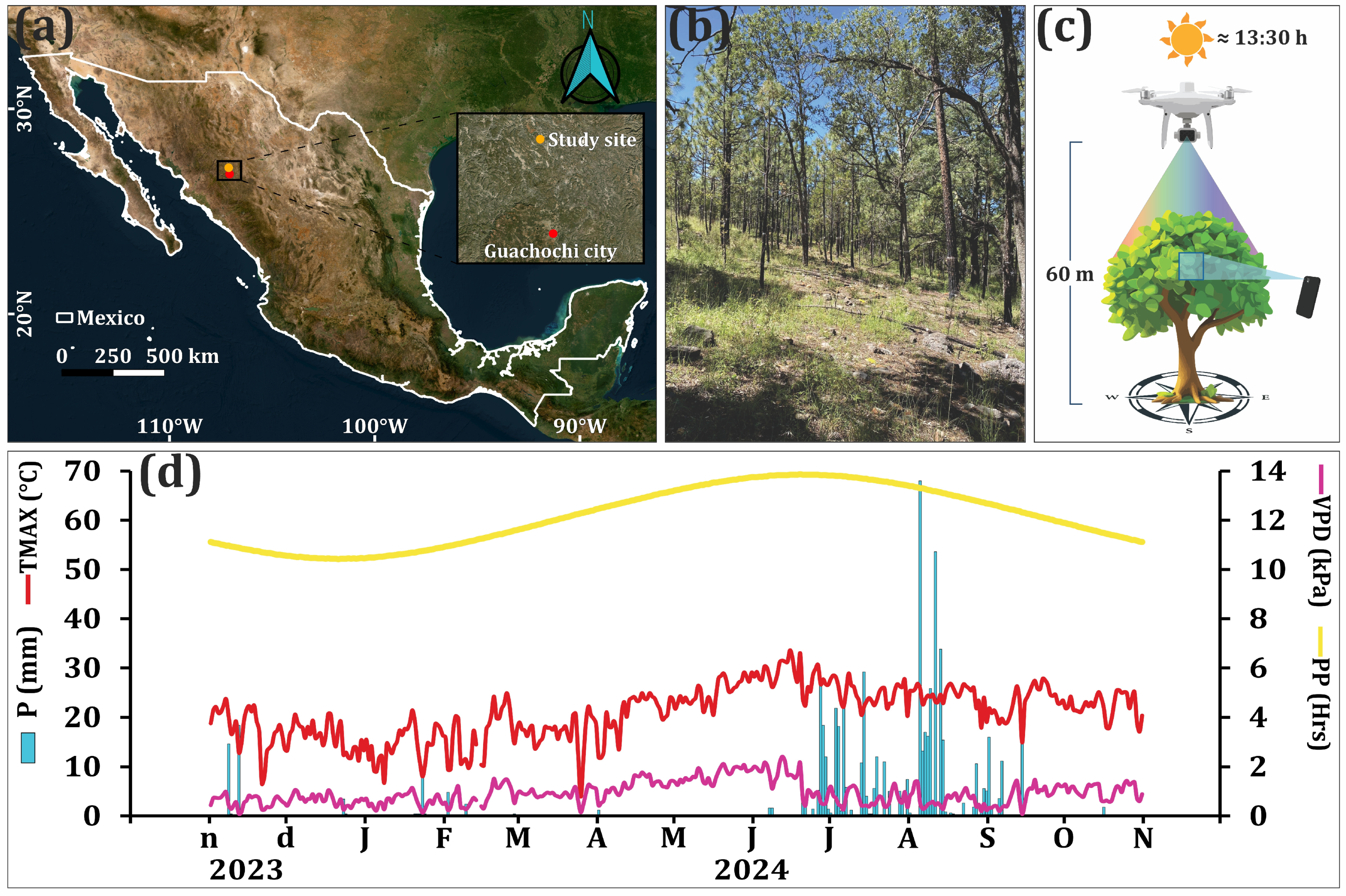
2.1. Study Area and Data Collection
2.2. Transitional Phenophases: Ground and Remote Sensing Detection
2.3. Environmental and Phenology Relationships
3. Results
3.1. Transitional Phenophases: Ground and Remote Sensing Detection
3.2. Environmental and Phenology Relationships
4. Discussion
4.1. Transitional Phenophases: Ground and Remote Sensing Detection
4.2. Environmental and Phenological Relationships
4.3. Final Remarks
4.4. Limitations
5. Conclusions
Supplementary Materials
Author Contributions
Funding
Data Availability Statement
Conflicts of Interest
Appendix A
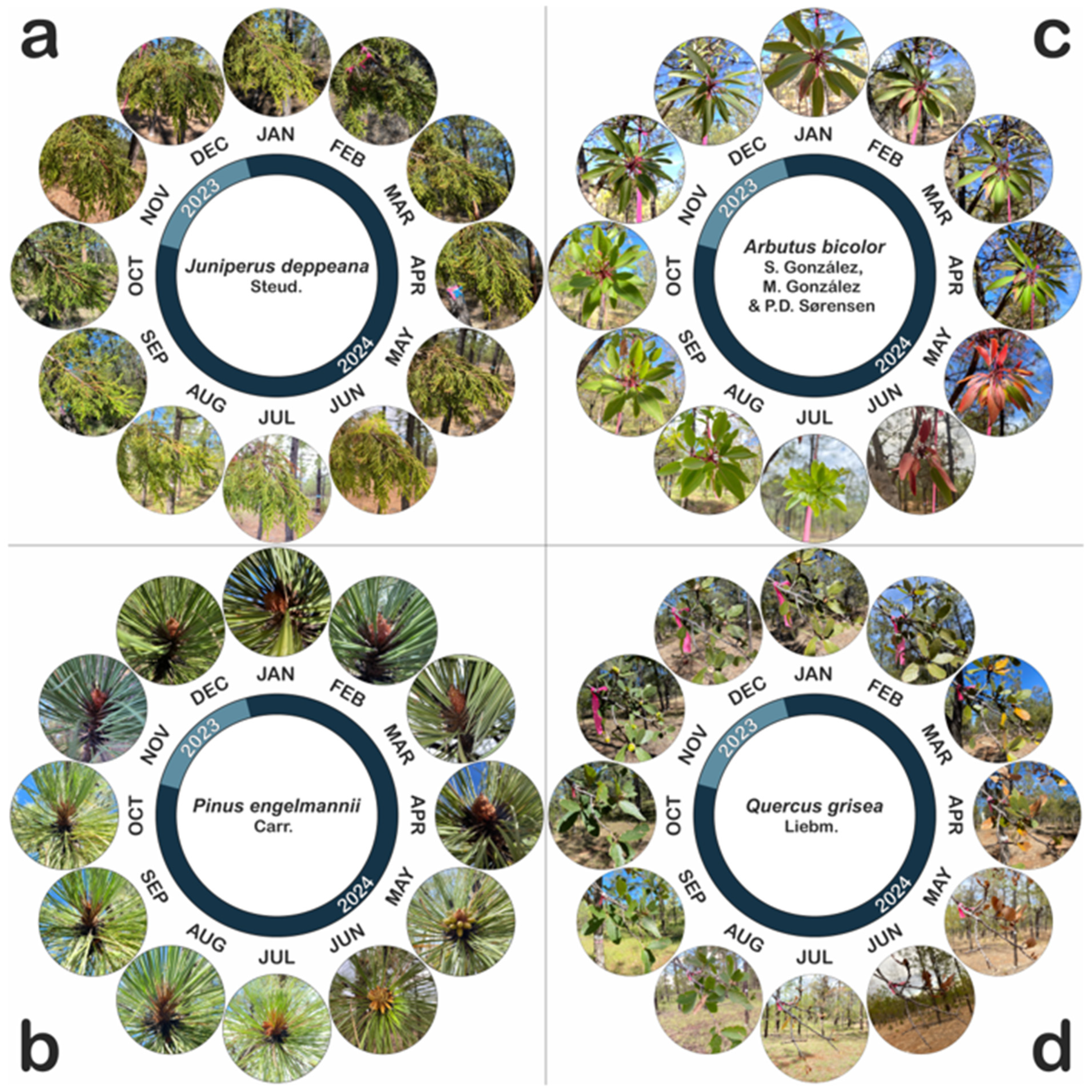
Appendix A.1. Ecology of the Studied Species
Appendix A.1.1. Arbutus bicolor S. González, M. González & P.D. Sørensen
Appendix A.1.2. Juniperus deppeana Steud.
Appendix A.1.3. Pinus engelmannii Carr.
Appendix A.1.4. Quercus grisea Liebm.
Appendix B

| Effect | F | Df | Df.res | Pr(>F) | Signif.Codes |
|---|---|---|---|---|---|
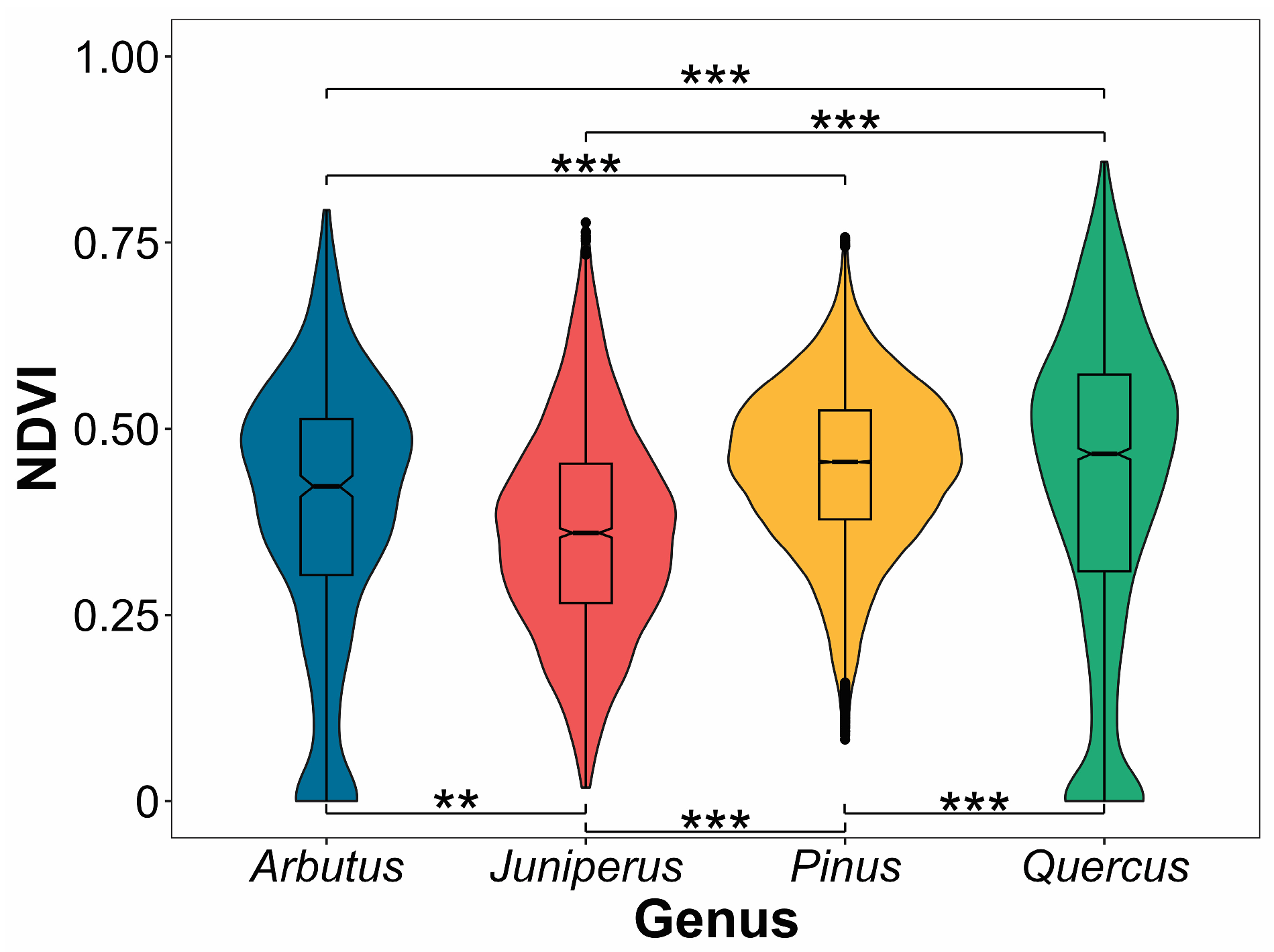
| Genus | 35.387 | 3 | 520 | <2.2 × 10⁻¹⁶ | *** |
| Date | 481.451 | 44 | 22717 | <2.2× 10⁻¹⁶ | *** |
| Interaction Genus × Date | 155.506 | 132 | 22717 | <2.2× 10⁻¹⁶ | *** |
| Comparison | n1 | n2 | Statistic | df | p | p.adj | Significance |
|---|---|---|---|---|---|---|---|
| Arbutus–Juniperus | 540 | 2310 | 3.22 | 694 | 1.00× 10−03 | 8.00 × 10−03 | ** |
| Arbutus–Pinus | 540 | 17,439 | −7.35 | 551 | 7.35 × 10⁻¹³ | 4.41 × 10⁻¹² | *** |
| Arbutus–Quercus | 540 | 3128 | −3.99 | 816 | 7.29 × 10−05 | 4.37 × 10−04 | *** |
| Juniperus–Pinus | 2310 | 17,439 | −28.1 | 2698 | 7.96 × 10−153 | 4.78 × 10−152 | *** |
| Juniperus–Quercus | 2310 | 3128 | −12.9 | 5363 | 1.95 × 10−37 | 1.17 × 10−36 | *** |
| Pinus–Quercus | 17,439 | 3128 | 5.94 | 3428 | 3.10 × 10−09 | 1.86 × 10−08 | *** |
| Effect | F | Df | Df.res | Pr(>F) | Signif.Codes |
|---|---|---|---|---|---|
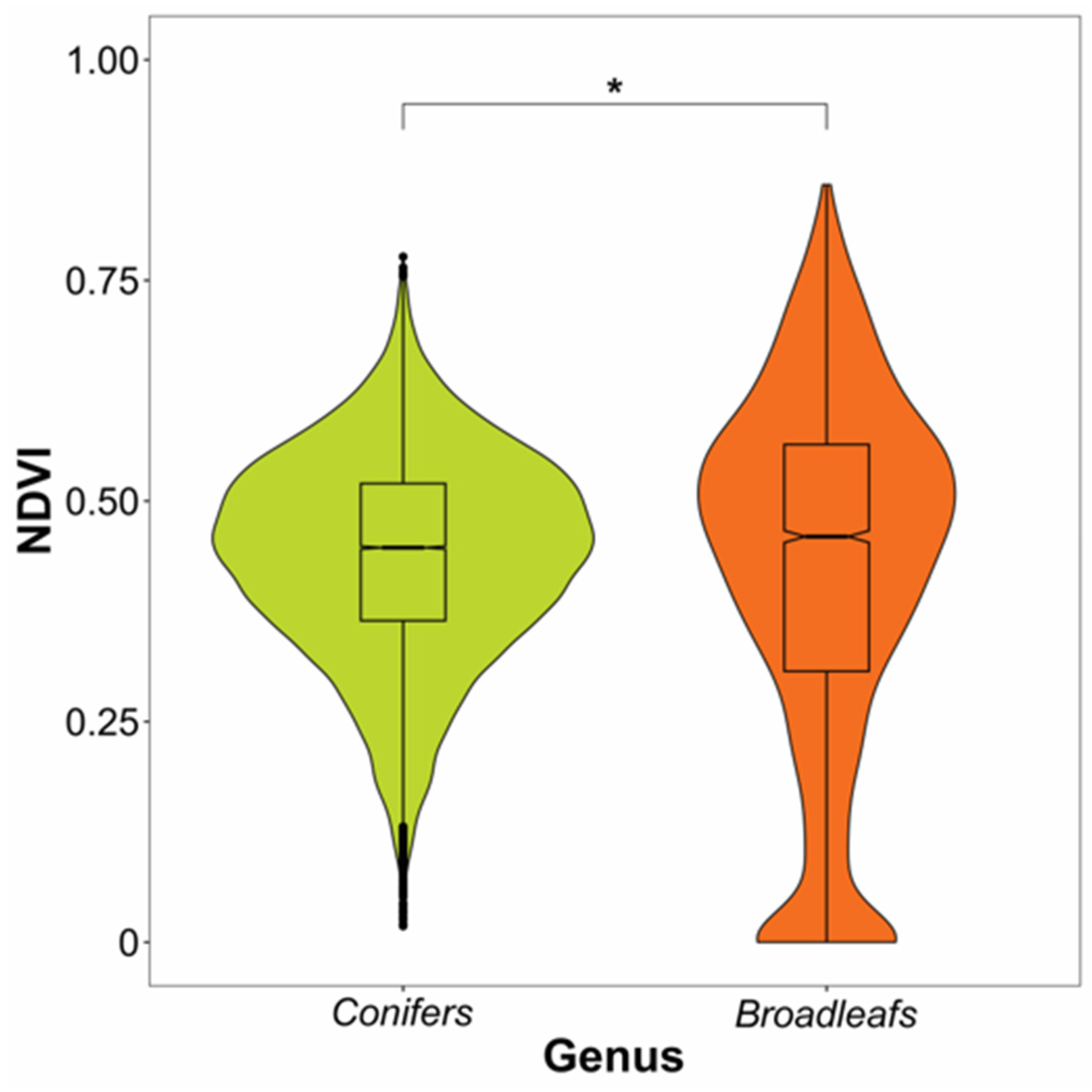
| Class (Conifer or Broadleaf) | 5.5412 | 1 | 522 | 0.01894 | * |
| Date | 458.0485 | 44 | 22,805 | <2.2 × 10⁻¹⁶ | *** |
| Interaction Class × Date | 416.686 | 44 | 22,805 | <2.2 × 10⁻¹⁶ | *** |
References
- Ault, T.R.; Schwartz, M.D.; Zurita-Milla, R.; Weltzin, J.F.; Betancourt, J.L. Trends and natural variability of spring onset in the coterminous United States as evaluated by a new gridded dataset of spring indices. J. Clim. 2015, 28, 8363–8378. [Google Scholar] [CrossRef]
- Keenan, T.F.; Gray, J.; Friedl, M.A.; Toomey, M.; Bohrer, G.; Hollinger, D.Y.; Munger, J.W.; O’Keefe, J.; Schmid, H.P.; Wing, I.S.; et al. Net carbon uptake has increased through warming-induced changes in temperate forest phenology. Nat. Clim. Change 2014, 4, 598–604. [Google Scholar] [CrossRef]
- Piao, S.; Liu, Z.; Wang, T.; Peng, S.; Ciais, P.; Huang, M.; Ahlstrom, A.; Burkhart, J.F.; Chevallier, F.; Janssens, I.A.; et al. Weakening temperature control on the interannual variations of spring carbon uptake across northern lands. Nat. Clim. Change 2017, 7, 359–363. [Google Scholar] [CrossRef]
- Piao, S.; Liu, Q.; Chen, A.; Janssens, I.A.; Fu, Y.; Dai, J.; Liu, L.; Lian, X.; Shen, M.; Zhu, X. Plant phenology and global climate change: Current progresses and challenges. Glob. Change Biol. 2019, 25, 1922–1940. [Google Scholar] [CrossRef] [PubMed]
- Klosterman, S.; Melaas, E.; Wang, J.A.; Martinez, A.; Frederick, S.; O’Keefe, J.; Orwig, D.A.; Wang, Z.; Sun, Q.; Schaaf, C.; et al. Fine-scale perspectives on landscape phenology from unmanned aerial vehicle (UAV) photography. Agric. For. Meteorol. 2018, 248, 397–407. [Google Scholar] [CrossRef]
- Park, J.Y.; Muller-Landau, H.C.; Lichstein, J.W.; Rifai, S.W.; Dandois, J.P.; Bohlman, S.A. Quantifying leaf phenology of individual trees and species in a tropical forest using Unmanned Aerial Vehicle (UAV) images. Remote Sens. 2019, 11, 1534. [Google Scholar] [CrossRef]
- Thapa, S.; Millan, V.E.G.; Eklundh, L. Assessing Forest Phenology: A multi-scale comparison of near-surface (UAV, spectral reflectance sensor, PhenoCam) and satellite (MODIS, Sentinel-2) remote sensing. Remote Sens. 2021, 13, 1597. [Google Scholar] [CrossRef]
- Fawcett, D.; Bennie, J.; Anderson, K. Monitoring spring phenology of individual tree crowns using drone-acquired NDVI data. Remote Sens. Ecol. Conserv. 2020, 7, 227–244. [Google Scholar] [CrossRef]
- Berra, E.F.; Gaulton, R.; Barr, S. Assessing spring phenology of a temperate woodland: A multiscale comparison of ground, unmanned aerial vehicle and Landsat satellite observations. Remote Sens. Environ. 2019, 223, 229–242. [Google Scholar] [CrossRef]
- Delpierre, N.; Vitasse, Y.; Chuine, I.; Guillemot, J.; Bazot, S.; Rutishauser, T.; Rathgeber, C.B.K. Temperate and boreal forest tree phenology: From organ-scale processes to terrestrial ecosystem models. Ann. For. Sci. 2016, 73, 5–25. [Google Scholar] [CrossRef]
- Bosio, F.; Rossi, S.; Marcati, C.R. Periodicity and environmental drivers of apical and lateral growth in a Cerrado woody species. Trees 2016, 30, 1495–1505. [Google Scholar] [CrossRef]
- Seager, R.; Ting, M.; Davis, M.; Cane, M.; Naik, N.; Nakamura, J.; Li, C.; Cook, E.; Stahle, D.W. Mexican drought: An observational modeling and tree ring study of variability and climate change. Atmósfera 2009, 22, 1–31. [Google Scholar]
- Silva-Ávila, N.; Pompa-García, M.; Martínez-Rivas, J.A. Kawí Tamiruyé: Un acceso universal al conocimiento del bosque. Una revisión documental. Nat. Soc. Desafíos Medioambient. 2025, 11, 60–75. [Google Scholar] [CrossRef]
- Klinger, Y.P.; Eckstein, R.L.; Kleinebecker, T. iPhenology: Using open-access citizen science photos to track phenology at continental scale. Methods Ecol. Evol. 2023, 14, 1424–1431. [Google Scholar] [CrossRef]
- Richardson, A.D.; Braswell, B.H.; Hollinger, D.Y.; Jenkins, J.P.; Ollinger, S.V. Near-surface remote sensing of spatial and temporal variation in canopy phenology. Ecol. Appl. 2009, 19, 1417–1428. [Google Scholar] [CrossRef]
- NASA POWER Data Access Viewer. Available online: https://power.larc.nasa.gov/data-access-viewer/ (accessed on 4 April 2025).
- NOAA Solar Calculator. Available online: https://gml.noaa.gov/grad/solcalc/ (accessed on 4 April 2025).
- Support for P4 Multispectral. Available online: https://www.dji.com/mx/support/product/p4-multispectral (accessed on 4 June 2025).
- Lin, C.; Chen, S.-Y.; Chen, C.-C.; Tai, C.-H. Detecting newly grown tree leaves from unmanned-aerial-vehicle images using hyperspectral target detection techniques. ISPRS J. Photogramm. Remote Sens. 2018, 142, 174–189. [Google Scholar] [CrossRef]
- Li, D.; Chen, J.M.; Zhang, X.; Yan, Y.; Zhu, J.; Zheng, H.; Zhou, K.; Yao, X.; Tian, Y.; Zhu, Y.; et al. Improved estimation of leaf chlorophyll content of row crops from canopy reflectance spectra through minimizing canopy structural effects and optimizing off-noon observation time. Remote Sens. Environ. 2020, 248, 111985. [Google Scholar] [CrossRef]
- OpenDroneMap. A Command Line Toolkit to Generate Maps, Point Clouds, 3D Models and Dems from Drone, Balloon or Kite Images. Available online: https://github.com/OpenDroneMap/ODM (accessed on 20 February 2025).
- R Core Team. R: A Language and Environment for Statistical Computing; The R Project for Statistical Computing: Vienna, Austria, 2025; Available online: https://www.R-project.org/ (accessed on 4 June 2025).
- Myers, L.; Sirois, M.J. Spearman Correlation Coefficients, Differences between. Wiley StatsRef Stat. Ref. Online, 2014; epub ahead of print. [Google Scholar] [CrossRef]
- Primack, R.B.; Laube, J.; Gallinat, A.S.; Menzel, A. From observations to experiments in phenology research: Investigating climate change impacts on trees and shrubs using dormant twigs. Ann. Bot. 2015, 116, 889–897. [Google Scholar] [CrossRef]
- Beaton, J.; Perry, A.; Cottrell, J.; Iason, G.; Stockan, J.; Cavers, S. Phenotypic trait variation in a long-term multisite common garden experiment of Scots pine in Scotland. Sci. Data 2022, 9, 671. [Google Scholar] [CrossRef]
- Wolkovich, E.M.; Cook, B.I.; Allen, J.M.; Crimmins, T.M.; Betancourt, J.L.; Travers, S.E.; Pau, S.; Regetz, J.; Davies, T.J.; Kraft, N.J.B.; et al. Warming experiments underpredict plant phenological responses to climate change. Nature 2012, 485, 494–497. [Google Scholar] [CrossRef]
- Delpierre, N.; Guillemot, J.; Dufrêne, E.; Cecchini, S.; Nicolas, M. Tree phenological ranks repeat from year to year and correlate with growth in temperate deciduous forests. Agric. For. Meteorol. 2017, 234–235, 1–10. [Google Scholar] [CrossRef]
- Stoy, P.C.; Williams, M.; Disney, M.; Prieto-Blanco, A.; Huntley, B.; Baxter, R.; Lewis, P. Upscaling as ecological information transfer: A simple framework with application to Arctic ecosystem carbon exchange. Landsc. Ecol. 2009, 24, 971–986. [Google Scholar] [CrossRef]
- Klosterman, S.T.; Hufkens, K.; Gray, J.M.; Melaas, E.; Sonnentag, O.; Lavine, I.; Mitchell, L.; Norman, R.; Friedl, M.A.; Richardson, A.D. Evaluating remote sensing of deciduous forest phenology at multiple spatial scales using PhenoCam imagery. Biogeosciences 2014, 11, 4305–4320. [Google Scholar] [CrossRef]
- Vitasse, Y.; Signarbieux, C.; Fu, Y.H. Global warming leads to more uniform spring phenology across elevations. Proc. Natl. Acad. Sci. USA 2018, 115, 1004–1008. [Google Scholar] [CrossRef]
- Jiang, D.; Xu, Z.; Nie, T. Advancements in monitoring tree phenology under global change: A comprehensive review. Forests 2025, 16, 771. [Google Scholar] [CrossRef]
- Richardson, A.D.; Black, T.A.; Ciais, P.; Delbart, N.; Friedl, M.A.; Gobron, N.; Hollinger, D.Y.; Kutsch, W.L.; Longdoz, B.; Luyssaert, S.; et al. Influence of spring and autumn phenological transitions on forest ecosystem productivity. Phil. Trans. R. Soc. B 2010, 365, 3227–3246. [Google Scholar] [CrossRef]
- Polgar, C.A.; Primack, R.B. Leaf-out phenology of temperate woody plants: From trees to ecosystems. New Phytol. 2011, 191, 926–941. [Google Scholar] [CrossRef]
- Vitasse, Y.; Bresson, C.C.; Kremer, A.; Michalet, R.; Delzon, S. Quantifying phenological plasticity to temperature in two temperate tree species. Funct. Ecol. 2010, 24, 1211–1218. [Google Scholar] [CrossRef]
- Walker, J.J.; Soulard, C.E. Phenology patterns indicate recovery trajectories of Ponderosa pine forests after high-severity fires. Remote Sens. 2019, 11, 2782. [Google Scholar] [CrossRef]
- White, K.; Pontius, J.; Schaberg, P. Remote sensing of spring phenology in northeastern forests: A comparison of methods, field metrics and sources of uncertainty. Remote Sens. Environ. 2014, 148, 97–107. [Google Scholar] [CrossRef]
- Ishii, H.; Asano, S. The role of crown architecture, leaf phenology and photosynthetic activity in promoting complementary use of light among coexisting species in temperate forests. Ecol. Res. 2010, 25, 715–722. [Google Scholar] [CrossRef]
- Hover, A.; Buissart, F.; Caraglio, Y.; Heinz, C.; Pailler, F.; Ramel, M.; Vennetier, M.; Prévosto, B.; Sabatier, S. Growth phenology in Pinus halepensis Mill.: Apical shoot bud content and shoot elongation. Ann. For. Sci. 2017, 74, 39. [Google Scholar] [CrossRef]
- Hallman, C.; Arnott, H. Morphological and physiological phenology of Pinus longaeva in the White Mountains of California. Tree-Ring Res. 2015, 71, 1–12. [Google Scholar] [CrossRef]
- Burdon, R.D. Shoot phenology as a driver or modulator of stem diameter growth and wood properties, with special reference to Pinus radiata. Forests 2023, 14, 570. [Google Scholar] [CrossRef]
- Basler, D.; Körner, C. Photoperiod and temperature responses of bud swelling and bud burst in four temperate forest tree species. Tree Physiol. 2014, 34, 377–388. [Google Scholar] [CrossRef]
- Man, Z.; Zhang, J.; Liu, J.; Liu, L.; Yang, J.; Cao, Z. Process-based modeling of phenology and radial growth in Pinus tabuliformis in response to climate factors over a cold and semi-arid region. Plants 2024, 13, 980. [Google Scholar] [CrossRef]
- Clark, J.S.; Salk, C.; Melillo, J.; Mohan, J. Tree phenology responses to winter chilling, spring warming, at north and south range limits. Funct. Ecol. 2014, 28, 1344–1355. [Google Scholar] [CrossRef]
- Acosta-Hernández, A.C.; Pompa-García, M.; Martínez-Rivas, J.A.; Vivar-Vivar, E.D. Cutting the Greenness Index into 12 monthly slices: How intra-annual NDVI dynamics help decipher drought responses in mixed forest tree species. Remote Sens. 2024, 16, 389. [Google Scholar] [CrossRef]
- Gunderson, C.A.; Edwards, N.T.; Walker, A.V.; O’Hara, K.H.; Campion, C.M.; Hanson, P.J. Forest phenology and a warmer climate—Growing season extension in relation to climatic provenance. Glob. Change Biol. 2011, 18, 2008–2025. [Google Scholar] [CrossRef]
- Luo, Y.; Zohner, C.; Crowther, T.W.; Feng, J.; Hoch, G.; Li, P.; Richardson, A.D.; Vitasse, Y.; Gessler, A. Internal physiological drivers of leaf development in trees: Understanding the relationship between non-structural carbohydrates and leaf phenology. Funct. Ecol. 2024, 1–14, early view. [Google Scholar] [CrossRef]
- Zhang, J.; Zhai, J.; Wang, J.; Si, J.; Li, J.; Ge, X.; Li, Z. Interrelationships and environmental influences of photosynthetic capacity and hydraulic conductivity in desert species Populus pruinose. Forests 2024, 15, 1094. [Google Scholar] [CrossRef]
- Gray, R.E.J.; Ewers, R.M. Monitoring forest phenology in a changing world. Forests 2021, 12, 297. [Google Scholar] [CrossRef]
- Kellomäki, S. Physiology, growth, and acclimatizing of boreal tree species to climate. In Management of Boreal Forests, 1st ed.; Springer: Cham, Switzerland, 2022; pp. 139–216. [Google Scholar] [CrossRef]
- Fu, Y.H.; Piao, S.; de Beeck, M.O.; Cong, N.; Zhao, H.; Zhang, Y.; Menzel, A.; Janssens, I.A. Recent spring phenology shifts in western Central Europe based on multiscale observations. Glob. Ecol. Biogeogr. 2014, 23, 1255–1263. [Google Scholar] [CrossRef]
- Fadón, E.; Fernandez, E.; Behn, H.; Luedeling, E. A conceptual framework for winter dormancy in deciduous trees. Agronomy 2020, 10, 241. [Google Scholar] [CrossRef]
- Wu, X.; Niu, C.; Liu, X.; Hu, T.; Feng, Y.; Zhao, Y.; Liu, S.; Liu, Z.; Dai, G.; Zhang, Y.; et al. Canopy structure regulates autumn phenology by mediating the microclimate in temperate forests. Nat. Clim. Change 2024, 14, 1299–1305. [Google Scholar] [CrossRef]
- Vitasse, Y.; Lenz, A.; Hoch, G.; Körner, C. Earlier leaf-out rather than difference in freezing resistance puts juvenile trees at greater risk of damage than adult trees. J. Ecol. 2014, 102, 981–988. [Google Scholar] [CrossRef]
- Radville, L.; Post, E.; Eissenstat, D.M. On the sensitivity of root and leaf phenology to warming in the Arctic. Arct. Antarct. Alp. Res. 2018, 50, S100020. [Google Scholar] [CrossRef]
- González-Elizondo, M.S.; González-Elizondo, M.; Sørensen, P.D. Arbutus bicolor (Ericaceae, Arbuteae), a new species from Mexico. Act. Bot. Mex. 2012, 99, 55–72. [Google Scholar] [CrossRef]
- Herrerías-Mier, L.G.; de Pascual Pola, M.C.C.N. Características estructurales y demográficas de Juniperus deppeana Steud. en dos localidades del estado de Tlaxcala. Rev. Mex. Cienc. For. 2021, 11, 124–151. [Google Scholar] [CrossRef]
- Jiménez-Salazar, M.A.; Méndez-González, J. Distribución actual y potencial de Pinus engelmannii Carriére bajo escenarios de cambio climático. Madera Bosques 2021, 27, e2732117. [Google Scholar] [CrossRef]
- Pavek, D.S. Pinus engelmannii. Fire Effects Information System [Online]. U.S. Department of Agriculture, Forest Service, Rocky Mountain Research Station, Fire Sciences Laboratory (Producer). 1994. Available online: https://www.fs.usda.gov/database/feis/plants/tree/pineng/all.html (accessed on 9 May 2025).
- Pavek, D.S. Quercus grisea. Fire Effects Information System [Online]. U.S. Department of Agriculture, Forest Service, Rocky Mountain Research Station, Fire Sciences Laboratory (Producer). 1994. Available online: https://www.fs.usda.gov/database/feis/plants/tree/quegri/all.html (accessed on 9 May 2025).
| Species | Variable | n | Min | Max | Mean | SD | Age |
|---|---|---|---|---|---|---|---|
| A. bicolor | BD (cm) | 5 | 16.30 | 31.50 | 21.66 | 5.83 | |
| DBH (cm) | 5 | 9.80 | 21.90 | 14.20 | 4.80 | ||
| CH (m) | 5 | 0.87 | 1.86 | 1.56 | 0.39 | 46 ± 4 | |
| TH (m) | 5 | 4.01 | 7.57 | 5.70 | 1.30 | ||
| J. deppeana | BD (cm) | 5 | 11.40 | 19.10 | 14.80 | 3.35 | |
| DBH (cm) | 5 | 8.10 | 12.00 | 9.86 | 1.89 | ||
| CH (m) | 5 | 1.95 | 2.06 | 1.99 | 0.05 | 45 ± 3 | |
| TH (m) | 5 | 4.07 | 4.67 | 4.27 | 0.27 | ||
| P. engelmannii | BD (cm) | 5 | 20.70 | 33.80 | 28.74 | 6.17 | |
| DBH (cm) | 5 | 16.30 | 27.50 | 23.20 | 5.18 | 60 ± 2 | |
| CH (m) | 5 | 2.49 | 3.02 | 2.75 | 0.21 | ||
| TH (m) | 5 | 7.31 | 12.20 | 10.14 | 1.93 | ||
| Q. grisea | BD (cm) | 5 | 23.70 | 40.30 | 33.54 | 6.67 | |
| DBH (cm) | 5 | 19.20 | 32.60 | 26.12 | 5.19 | ||
| CH (m) | 5 | 2.46 | 3.00 | 2.77 | 0.22 | 42 ± 1 | |
| TH (m) | 5 | 9.71 | 12.82 | 11.65 | 1.20 |
| Phenophase | Period | Variables | Model | R2 |
|---|---|---|---|---|
| 1 | 15 November 2023 to 15 February 2024 (Late autumn–winter) | Juniperus–PP | NDVI = −0.08 × PP + 1.09 | 0.63 |
| Pinus–PP | NDVI = −0.06 × PP + 1.08 | 0.62 | ||
| 2 | 15 February 2024 to 14 June 2024 (Late winter–spring) | Quercus–PP | NDVI = −0.14 × PP + 2.08 | 0.80 |
| Quercus–TMAX | NDVI = −0.02 × TMAX + 0.71 | 0.66 | ||
| Quercus–VPD | NDVI = −0.22 × VPD + 0.56 | 0.64 | ||
| 3 | 14 June 2024 to 14 October 2024 (Summer–early autumn) | Juniperus–PP | NDVI = 0.08 × PP − 0.68 | 0.93 |
| Juniperus–TMAX | NDVI = 0.01 × TMAX + 0.003 | 0.58 | ||
| Juniperus–VPD | NDVI = 0.09 × VPD + 0.24 | 0.57 |
Disclaimer/Publisher’s Note: The statements, opinions and data contained in all publications are solely those of the individual author(s) and contributor(s) and not of MDPI and/or the editor(s). MDPI and/or the editor(s) disclaim responsibility for any injury to people or property resulting from any ideas, methods, instructions or products referred to in the content. |
© 2025 by the authors. Licensee MDPI, Basel, Switzerland. This article is an open access article distributed under the terms and conditions of the Creative Commons Attribution (CC BY) license (https://creativecommons.org/licenses/by/4.0/).
Share and Cite
Pompa-García, M.; Vivar-Vivar, E.D.; Acosta-Hernández, A.C.; Rossi, S. The Phenophases of Mixed-Forest Species Are Regulated by Photo-Hydro-Thermal Conditions: An Approach Using UAV-Derived and In Situ Data. Forests 2025, 16, 1118. https://doi.org/10.3390/f16071118
Pompa-García M, Vivar-Vivar ED, Acosta-Hernández AC, Rossi S. The Phenophases of Mixed-Forest Species Are Regulated by Photo-Hydro-Thermal Conditions: An Approach Using UAV-Derived and In Situ Data. Forests. 2025; 16(7):1118. https://doi.org/10.3390/f16071118
Chicago/Turabian StylePompa-García, Marín, Eduardo Daniel Vivar-Vivar, Andrea Cecilia Acosta-Hernández, and Sergio Rossi. 2025. "The Phenophases of Mixed-Forest Species Are Regulated by Photo-Hydro-Thermal Conditions: An Approach Using UAV-Derived and In Situ Data" Forests 16, no. 7: 1118. https://doi.org/10.3390/f16071118
APA StylePompa-García, M., Vivar-Vivar, E. D., Acosta-Hernández, A. C., & Rossi, S. (2025). The Phenophases of Mixed-Forest Species Are Regulated by Photo-Hydro-Thermal Conditions: An Approach Using UAV-Derived and In Situ Data. Forests, 16(7), 1118. https://doi.org/10.3390/f16071118