Abstract
Accurate real-time tracking of forest fires using UAV platforms is crucial for timely early warning, reliable spread prediction, and effective autonomous suppression. Existing detection-based multi-object tracking methods face challenges in accurately associating targets and maintaining smooth tracking trajectories in complex forest environments. These difficulties stem from the highly nonlinear movement of flames relative to the observing UAV and the lack of robust fire-specific feature modeling. To address these challenges, we introduce AO-OCSORT, an association-optimized observation-centric tracking framework designed to enhance robustness in dynamic fire scenarios. AO-OCSORT builds on the YOLOX detector. To associate detection results across frames and form smooth trajectories, we propose a temporal–physical similarity metric that utilizes temporal information from the short-term motion of targets and incorporates physical flame characteristics derived from optical flow and contours. Subsequently, scene classification and low-score filtering are employed to develop a hierarchical association strategy, reducing the impact of false detections and interfering objects. Additionally, a virtual trajectory generation module is proposed, employing a kinematic model to maintain trajectory continuity during flame occlusion. Locally evaluated on the 1080P-resolution FireMOT UAV wildfire dataset, AO-OCSORT achieves a 5.4% improvement in MOTA over advanced baselines at 28.1 FPS, meeting real-time requirements. This improvement enhances the reliability of fire front localization, which is crucial for forest fire management. Furthermore, AO-OCSORT demonstrates strong generalization, achieving 41.4% MOTA on VisDrone, 80.9% on MOT17, and 92.2% MOTA on DanceTrack.
1. Introduction
Forests are a vital component of Earth’s ecosystem, playing a crucial role in maintaining ecological balance and supporting life [1]. However, forest fires occur frequently each year, triggered by both natural factors, such as global warming, dry winter climates, and lightning strikes, and anthropogenic activities, including unattended ignition sources, careless use of fire, and littering [2]. These fires pose significant threats to nature, human life, and property. Consequently, the early detection and tracking of forest fires have become urgent necessities. Traditional forest fire monitoring systems include manual patrols, watchtower observations, sensor networks, and satellite remote sensing. Historically, fire monitoring and suppression efforts have been human-driven, relying on forest rangers patrolling designated routes and watchtower surveillance for fire detection, followed by the manual development of suppression plans [3]. This approach suffers from limited coverage, delayed responses, and significant safety risks for personnel. Additionally, maintaining sensor-based detection systems incurs substantial costs, often encountering issues such as power shortages or communication interruptions. The early stage of a fire, characterized by smoke and flame generation, is crucial for early warning and intervention. Satellite remote sensing, typically employed for large-scale monitoring, struggles to detect localized areas and small-scale fires in their early stages. Recently, unmanned aerial vehicle (UAV) technology has garnered significant attention for forest fire monitoring due to its flexibility, mobility, and cost-effectiveness for wide-area coverage. UAV-based fire monitoring offers distinct advantages over manual methods: (1) significantly broader monitoring coverage; (2) more flexible patrol path planning; (3) potential for fire spread prediction using tracking technology during fire progression; and (4) the possibility of direct fire suppression at ignition points with UAVs equipped with tracking-guided systems, thereby preventing fire spread and reducing personnel safety risks.
In the realm of UAV-based monitoring, multi-object tracking (MOT) within computer vision [4,5,6,7,8] has become indispensable for navigation, autonomous fire suppression, and fire spread estimation. Although advanced MOT algorithms such as DeepSORT [9], ByteTrack [10], and OC-SORT [11] demonstrate significant stability, accuracy, and real-time processing capabilities under general conditions [12,13,14], forest fire tracking presents distinct challenges: (1) Highly Nonlinear Dynamics. The interaction between flame and UAV movement leads to complex, nonlinear trajectories that traditional linear motion models—such as Kalman Filters [15], which are often used in trackers [9,11,16]—cannot effectively capture due to their single-step linear prediction assumptions [17]. (2) Severe Appearance Ambiguity and Distortion. Motion blur caused by flames and the inherent visual similarity among fire points result in frequent trajectory ambiguities, target misidentification, identity switches, and fragmented tracks. Current MOT approaches, which predominantly depend on linear association strategies and general appearance features, inadequately model the specific attributes of fire and fail to effectively differentiate visually similar targets in chaotic environments.
To alleviate the above problems, efforts in research on fire tracking have predominantly concentrated on two areas: feature extraction and the optimization of tracking frameworks. In terms of feature extraction, Xie et al. [18] developed a method for flame segmentation and tracking within the YCbCr color space, while Khalil et al. [19] employed multi-color space analysis combined with background modeling. For tracking framework optimization, Rong et al. [20] proposed a cumulative geometric independent component analysis (C-GICA) model featuring a delayed data structure to track flame spread dynamics. Yuan et al. [21] designed a UAV-based system utilizing image processing techniques such as color space conversion and thresholding. Daoud et al. [22] integrated an enhanced YOLOv3 [23] with Kalman filtering, while Yuan et al. [24] employed histogram segmentation and optical flow methodologies. Cai et al. [25] combined an improved Gaussian mixture model (GMM) with mean shift, and Mouelhi et al. [26] implemented a hybrid geodesic active contour (GAC) model. Additionally, De et al. [27] refined YOLOv4 [28] for enhanced fire monitoring. Despite progress in controlled settings, these approaches still fail to effectively handle the nonlinear trajectories of dynamic fire progression, resulting in tracking inaccuracies such as identity confusion between adjacent flames, misidentifications, and missed detections under challenging conditions. The complexity inherent in forest fire scenarios poses ongoing challenges for future monitoring and mitigation efforts.
Addressing these limitations requires a fundamental enhancement of the tracker’s ability to model complex temporal dynamics and fire-specific features. Recent developments in state-space models (SSMs) [29], particularly the Mamba architecture [30], have shown remarkable efficacy in long-sequence modeling due to their selective scan mechanism and hardware-aware computation strategy. These models have been widely used in downstream tasks that require long-term and complex sequence understanding capabilities. Inspired by these capabilities, we incorporate Mamba into the multiple object tracking (MOT) framework to more effectively capture the intricate temporal evolution of fire trajectories along with frame-specific physical features.
Building upon the YOLOX detector [31], this paper proposes an association optimization method to enhance the observation-centric simple online real-time tracker (OCSORT) [11], termed AO-OCSORT. As a deep learning-based object detection algorithm, YOLOX excels in rapidly and accurately identifying objects within images. For the detection results generated by YOLOX, the OC-SORT MOT method establishes cross-frame target trajectories through data association and track management mechanisms, effectively reducing cumulative errors and improving adaptability in complex scenarios. However, OC-SORT lacks robust modeling capability for fire-related objects, exhibiting limitations in analyzing visually ambiguous and highly similar flame objects. Consequently, AO-OCSORT optimizes the data association stage by modeling complex temporal dynamics and fire-specific characteristics. To mitigate the scarcity of comprehensive forest fire datasets, we curated aerial video imagery of forest canopies. Data selection prioritized diverse challenging scenarios—including varying illumination, vegetation interference, and complex viewing angles—to ensure dataset representativeness. These images were processed to analyze complex features such as smoke and flames, enabling the development of a dedicated fire-tracking model for forest monitoring and warning systems.
The contributions of AO-OCSORT are summarized as follows:
- Introduction of a temporal–physical similarity metric, implemented through novel temporal correlation (TC) and physical feature modeling (PFM) components, which enhance target representation efficacy and association robustness in dynamic fire environments characterized by nonlinear motion and high visual similarity.
- Development of a hierarchical association strategy (HAS) that balances tracking accuracy gains from the joint metric with computational efficiency, integrating an adaptive threshold mechanism to reduce detection noise and bolster system robustness.
- Creation of a virtual trajectory generation (VTG) method designed to address detection inaccuracies and interruptions caused by flame dynamics and complex motion patterns in forest fire scenarios, ensuring continuity in tracking under environmental disturbances.
- Introduction of the AO-OCSORT framework alongside a specialized FireMOT forest fire-tracking dataset. Extensive experiments validate the model’s superior tracking stability on FireMOT, with its generalization performance further examined across three standard benchmark datasets.
2. Materials and Methods
2.1. Dataset
High-quality datasets are crucial for effectively evaluating the performance of forest fire-tracking models. The FireMOT dataset, introduced in this paper, primarily comprises publicly available aerial footage and fire videos sourced from online platforms. All videos are in visible light with a resolution of . It includes various challenges encountered in forest fire scenarios, such as different environments (e.g., snow-covered terrain, broadleaf forests, and coniferous forests) and complex factors, like illumination variations, viewpoint shifts, vegetation occlusion, and smoke interference, as depicted in Figure 1. This diversity enables a comprehensive assessment of the effectiveness and robustness of forest fire-tracking algorithms in complex real-world settings.
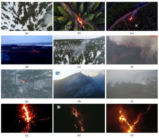
Figure 1.
Typical forest fire images from the FireMOT dataset. We describe the images in terms of the camera viewpoint, time of day, fire and smoke intensity, scene, etc. (a) Top-Down Shot, snow, daylight, minor fire, slight smoke. (b) Top-Down Shot, daylight, open flame, no visible smoke. (c) Top-Down Shot, dusk or dawn, minor fire, slight Smoke. (d) Oblique shot, dusk or dawn, minor fire, slight smoke. (e) Oblique shot, snow, daylight, minor fire, slight smoke. (f) Oblique shot, daylight, major fire, dense smoke. (g) Eye-Level shot, daylight, minor fire, medium smoke. (h) Oblique shot, dusk or dawn, minor fire, dense smoke. (i) Oblique shot, daylight, dense smoke, no active fire. (j) Oblique shot, night, major fire, no visible smoke. (k) Eye-Level shot, night, moderate fire, medium smoke. (l) Oblique shot, daylight, major fire, medium smoke.
The dataset is annotated using the well-established DarkLabel software (version 2.4) in accordance with the standard MOT format. Annotations comprise frame numbers, unique target identifiers (IDs), and bounding box coordinates. Video sequences are processed frame-by-frame during annotation, with all visible fire targets manually labeled. To improve efficiency, DarkLabel’s auto-prediction function is used, which estimates target positions based on previous frames. After annotation, comprehensive data files containing all target trajectories are created for subsequent tracking algorithm research and testing.
To guarantee the quality of annotation, explicit labeling protocols are established. Completely obscured targets are omitted, while partially occluded flames are annotated solely in their visible sections. Microscopic flames, indistinguishable to the naked eye, are excluded until they become clearly observable. Due to the inherent subjectivity of manual annotation, all labeled data underwent thorough verification to ensure accuracy, and only verified data were included in the final dataset.
Ultimately, the FireMOT dataset—comprising 60 video sequences encompassing the aforementioned forest scenarios and challenges—is curated through systematic data collection, screening, and stringent annotation verification. The dataset is evenly divided into training and test sets, with a 1:1 ratio. The training set contains 120,838 identity-annotated bounding boxes. Table 1 compares key metrics of FireMOT with mainstream MOT datasets.

Table 1.
Basic information about the FireMOT dataset.
To robustly assess the generalization capabilities of our method in similarity scenarios, we strategically employ three complementary benchmarks: (1) VisDrone [12] offers a critical UAV perspective, characterized by small targets and varied environmental conditions such as changes in illumination and weather. (2) MOT17 [13] presents challenges related to extreme occlusions in dense crowds, demanding robust detector performance. (3) DanceTrack [14] evaluates the modeling of nonlinear motion through complex, coordinated movements that defy linear assumptions. This triad intentionally targets key generalization aspects relevant to forest fire tracking, such as drone-specific conditions, severe occlusions, and nonlinear dynamics, while ensuring domain relevance.
2.2. Overall Framework
The proposed AO-OCSORT framework aligns with the detection-based MOT paradigm [11]. This approach involves decomposing videos into sequential frames, where target objects are identified within each individual frame to facilitate tracking. In this paradigm, for two consecutive frames, MOT is formulated as a matching problem between detection boxes in the current frame and target trajectories from the previous frame, as illustrated in Figure 2. The architecture of AO-OCSORT comprises four core components: a detector, a motion model, a data association module, and a trajectory manager. The workflow for tracking unfolds as follows.
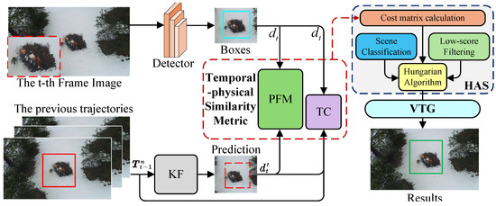
Figure 2.
The architecture of the AO-OCSORT framework. The AO-OCSORT algorithm associates existing trajectories with current detection bounding boxes. The proposed temporal–physical similarity metric integrates both temporal information and physical characteristics of fire targets to enhance data association. This information is processed by the HAS module, which uses scene classification and low-score filtering to reduce interference. Ultimately, the VTG module produces continuous and stable tracking trajectories.
The detector initially generates bounding boxes from the input image at frame t. YOLOX [31] is utilized as the detector. Each tracked trajectory represents a sequence of historical target states over n frames (e.g., position and scale).
During data association, detection boxes are matched with existing trajectories. For each detection and a possible trajectory, the Kalman filter (KF), functioning as the motion model, forecasts the trajectory’s current state , estimating the target’s position in frame t. The predicted box is subsequently compared with using intersection over union (IoU) to create a cost matrix that quantifies their affinity.
To address complex nonlinear dynamics, our temporal–physical similarity metric utilizes , , and as input variables. The temporal correlation (TC) component calculates a temporal similarity score based on and using a bidirectional Mamba architecture [30] to construct its encoder. This encoder extracts intricate motion features from nonlinear trajectories, enabling the decoder to effectively differentiate between correct and incorrect associations. Meanwhile, physical feature modeling (PFM) assesses the physical similarity by analyzing and . The region of interest (RoI) method [32] is employed to extract the object image delineated by the trajectory and the detection box. Subsequently, PFM analyzes the distinctive flame characteristics of the RoI image, thereby bolstering its capability to resist visually similar interference sources. This temporal–physical similarity produces an auxiliary cost matrix.
Computing cost matrices for all trajectory–detection pairs is inefficient. To address this issue, we propose a hierarchical association strategy (HAS) for group-based matching, which balances precision and efficiency. Scene classification and low-score filtering enhance the grouping process by minimizing false alarms and noise. The Hungarian algorithm [9] is employed to assign unique matches based on the computed cost matrices, thereby completing the data association process.
Trajectory management utilizes a state machine design [10], classifying trajectories into three categories: Active (continuously matched and updated with high confidence), Inactive (unmatched but recoverable within a tolerance window), and Lost (removed after consecutive mismatches). A five-frame historical state sequence, which includes position and motion, is maintained for each trajectory to support TC’s temporal modeling. To address tracking discontinuities arising from detection gaps, such as occlusion, motion blur, or dynamic interference, the virtual trajectory generation (VTG) module refines trajectories through motion interpolation and a dual-verification mechanism, compensating for missed detections and ensuring consistency. This process outputs the final tracking results for frame t, and the loop is repeated to maintain continuous tracking.
2.3. Temporal–Physical Similarity Metric
To address the challenges posed by complex flame dynamics and environmental interference, this paper introduces a temporal–physical similarity metric for data association, comprising temporal correlation and physical feature modeling.
2.3.1. Temporal Correlation
The structure of temporal correlation (TC), as depicted in Figure 3, aims to characterize temporal relationships by quantifying the associations between detection and trajectory . This module comprises two phases: temporal information encoding and motion decoding.
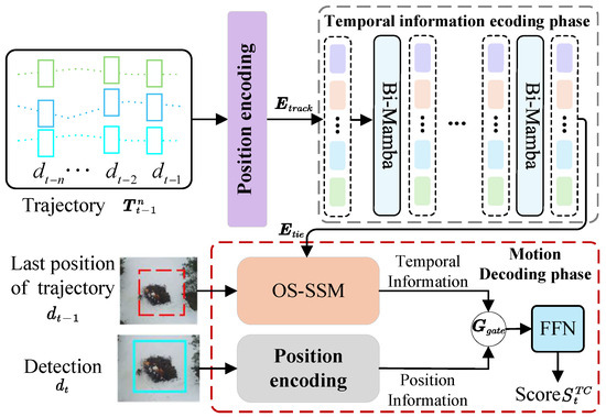
Figure 3.
Structure of the temporal correlation module. The initial encoding of temporal information involves extracting temporal features from trajectory sequences. Motion decoding begins by updating trajectory states with these encoded features and the target’s last known position, utilizing the OS-SSM approach. A gating mechanism and FFN then calculate the similarity score between trajectories and current detections, using the updated temporal information and position.
- (1)
- Temporal information encoding phase.
Given an object trajectory , the cosine position encoding method [33] is employed to derive the spatial coordinates and differential motion parameters for each element of the trajectory. This process generates a descriptor vector , where , , , and . The descriptor vectors from the n-frame historical trajectory are aggregated into a motion descriptor . represents the motion characteristics of the observed trajectory, which is subsequently processed by a linear layer to generate an embedded sequence .
The embedded sequence is then bidirectionally encoded using the temporal information encoding network. As illustrated in Figure 4, it efficiently leverages temporal information from continuous target trajectories by integrating multiple bi-Mamba architectures [30]. Each bidirectional Mamba layer utilizes two independent Mamba structures to process temporal information via forward and backward propagation, respectively.
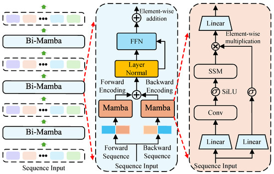
Figure 4.
Structure of the temporal information encoding network. Unfold the components of encoding network, bi-Mamba and Mamba sequentially from left to right.
During feature updates, and maintain the forward and reverse sequences of , respectively. To simplify the formula representation, we omit layer normalization and the feed-forward network (FFN) layer [34] for output features. The Mamba architecture, designed for long-range modeling of trajectory features, is illustrated in the middle part of Figure 4.
The Mamba architecture [30] captures temporal information through state-space models (SSMs) [29]. The updated sequence features are then output through an additional linear layer. State-space models (SSMs) are mathematical constructs used to characterize and analyze dynamic systems. By employing an SSM, the subsequent state of a system can be predicted based on its inputs, thereby facilitating deep sequence modeling. At time step , an SSM maps an input to an output via a hidden state . This system is governed by the following linear ordinary differential equation:
The learned parameters , , and govern system behavior. Here, evolution parameter determines the decay rate of the previous hidden state . In practice, deep learning algorithms handle discrete data, such as text, image blocks, and trajectory sequences. Therefore, the continuous parameters and are discretized using zero-order hold (ZOH). In the SSM [29] model, the continuous parameters are decomposed into discrete parameters and . These equations form a recurrence. At each step, the SSM combines the hidden state from the previous time step and the current input to produce a new hidden state .
As illustrated in the right section of Figure 4, the input sequence is transformed through linear and 1D convolution operations, followed by the application of a SiLU activation function. Subsequently, the SSM processes to generate the input matrix , the output matrix , and the time scale parameter :
Then, using the ZOH technique and the parameter Δ, discretize the parameters and to obtain and . According to Equation (2), the SSM can obtain the output .
Through iterative multi-layer bidirectional encoding, this phase outputs temporal encoding features , holistically capturing long-range dependencies and motion information within trajectories.
- (2)
- Motion decoding phase.
The motion decoding phase estimates the correlation between the trajectory and detection box using temporal encoding features . As depicted in Figure 5, the decoder structure utilizes inputs including the detection bounding box and the trajectory’s previous position . Initially, cosine positional encoding transforms into a high-dimensional space, yielding positional embeddings to enhance the model’s spatial awareness. Subsequently, these trajectory positional embeddings undergo processing by a linear layer and are partitioned along the channel dimension to extract positional features and their residual .
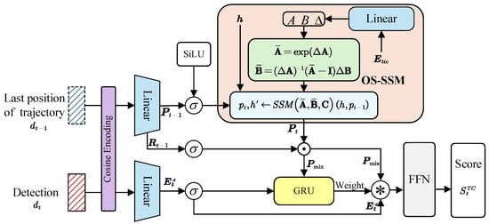
Figure 5.
Structure of the motion decoding network. The final positions of the input trajectory and the current detection box are encoded positionally and transformed into feature embeddings through two linear layers. The trajectory feature embedding, denoted as , is managed by the OS-SSM to forecast its temporal dynamics, resulting in trajectory prediction features, . A gating mechanism, governed by a GRU unit, adjusts the fusion ratio between and adaptively. The fusion process diagram is represented by an *. The fused features are processed through an FFN to estimate the temporal similarity score.
The feature is fed into the one-step SSM (OS-SSM) [35], which utilizes temporal modeling to produce trajectory prediction features . The historical positional data, , serves as a guide for generating the parametric matrix.
Following discretization, the transformation of the input position into the state is facilitated by the time sequence encoding feature and the input’s historical hidden state . The embedding of feature information from the current position to the next, which contains the state information, is accomplished in a single step.
Meanwhile, undergoes residual processing, whereby it is first transformed nonlinearly through an activation layer and subsequently multiplied by , integrating historical motion and positional data to produce the hybrid features .
Next, the vector is concatenated with the detection features . A gated mechanism, as described by [36], adaptively assigns weights to this concatenated vector.
The regulation weight generated by the GRU unit is denoted as . The concatenated features are weighted, fused, and then fed into an FFN for classification, resulting in confidence scores for matching target trajectory detection to bounding boxes, denoted as . The TC module is trained using the detection boxes and trajectories present in the training set. A binary cross-entropy loss function is utilized to predict whether a detection belongs to the trajectory .
2.3.2. Physical Feature Modeling
In addition to analyzing the relationship between trajectory and detection box using temporal information, we considered the flame’s physical characteristics to minimize background interference. The structural framework of the physical feature modeling module is depicted in Figure 6. This module receives frame images and flame-detection bounding boxes as inputs. The region of interest (RoI) method [32] extracts candidate areas from the input image based on . Subsequently, the RGB image of the RoIs is transformed into HSV color space, , to enhance flame target processing. An empirically determined HSV range for flames is applied to generate color masks, denoted as , allowing flame color filtering following the color space conversion.
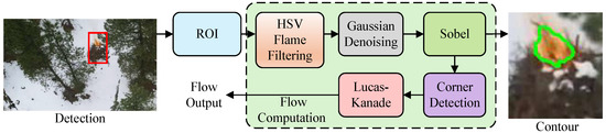
Figure 6.
Structure of physical feature modeling. ROI extraction is used to obtain image patches from objects within detection bounding boxes. The image is then converted to the HSV color space and processed with flame filtering and Gaussian denoising techniques. Contours are extracted using the Sobel operator, and corner detection is performed on these contours to compute sparse optical flow, which models the physical characteristics.
Following the application of the filtering operation to the image , Gaussian denoising is performed to suppress noise and prepare the data for subsequent processing. The denoised image is obtained through convolution:
where represents the Gaussian kernel. Subsequently, Sobel operators are applied to the denoised image to detect contours. The gradient magnitude G and direction are calculated as follows:
where and are the horizontal and vertical gradient magnitudes, respectively. Following this, non-maximum suppression is applied to generate contours. The resultant edge map is transformed into a binary mask, denoted as . Feature points on the edge mask are extracted using Shi–Tomasi corner detection, which is further used to compute optical flow coefficients using the Lucas–Kanade method.
where is the spatial gradient matrix and is the temporal gradient matrix.
The PFM utilizes contour information to quantify target shapes and optical flow data to evaluate the diffusion dynamics of flame targets, thereby establishing a physical model of flame behavior. A quantitative assessment of the alignment between target characteristics and trajectory patterns is generated at the physical feature level. A similar method is used to obtain optical flow and contour features for the final position of the trajectory. Cosine similarity is applied to generate scores, and , for two physical properties. By integrating temporal modeling of TC, the proposed temporal–physical similarity metric is incorporated into the HAS to guide the association process, enabling precise differentiation of flame targets through feature-driven constraints.
2.4. Hierarchical Association Strategy
According to [11], the primary challenge in data association is effectively matching object trajectories with detection boxes using a cost matrix. This model synthesizes three distinct matrices to form the cost matrix: (1) the overlap matrix, which is derived from the IoU between object predictions generated by motion models and detection boxes; (2) the momentum matrix, calculated based on the observed centroid momentum; and (3) the similarity matrix, obtained through the temporal–physical similarity metric.
where the matrix represents the estimated state of targets generated by trajectories, while Z denotes the state matrix of current detections. The matrix V encodes the direction of existing trajectories, calculated from observations across two consecutive time steps. The function computes the IoU between detection boxes and predicted states. The function evaluates directional consistency through momentum, considering both the trajectory’s inherent direction and the direction formed between its last position and new detections. Additionally, assesses temporal and physical attributes by aggregating similarities , , and . These metrics of temporal and physical similarity enhance flame target-tracking performance.
The Hungarian algorithm [9] is utilized with the aforementioned cost matrix to perform unique matching between trajectories and new detections. However, calculating the cost between all trajectories and detection boxes results in quadratic complexity, which elevates computational demands and subsequently hinders inference speed. To mitigate this, we propose a hierarchical association strategy (HAS) that organizes matching computations according to specific attributes, thus avoiding pairwise processing between trajectories and detection boxes. This strategy minimizes interference from low-confidence detections while maintaining a balance between optimizing model accuracy and enhancing computational efficiency. The structure of this strategy is illustrated in Figure 7.
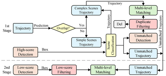
Figure 7.
Structure of the hierarchical association strategy. The HAS categorizes data associations into high-score and low-score groups. Scene classification segregates simple trajectories and high-score detections for prioritized matching, using only the IoU cost matrix to improve processing speed. For complex trajectories and low-score detections, a multi-level matching strategy is implemented to leverage additional spatiotemporal cues.
The association matching process takes as inputs the detection boxes from the current frame, , and trajectories from the previous frame, . Building upon a two-stage strategy similar to that presented in [10], we integrate key threshold controls for effective fire tracking: as the high detection confidence threshold, as the scene classification threshold, as the duplicate filtering threshold, and as the dynamic filtering threshold. The process yields the association results. For each video frame, detection boxes are initially segregated into and according to , initiating a staged association workflow.
- (1)
- The First Stage.
The scene classification delineates existing trajectories. Motion models produce predicted positions for all trajectories. When the IoU between predicted positions of two trajectories falls below 0, they are marked as overlapping. Overlapping trajectories are categorized as complex-scene trajectories, denoted as . For simple trajectories, represented as , association uses only the term in the cost matrix along with high-score detection boxes . Here, if the IoU between and falls below the threshold , the trajectory is identified as belonging to a nonlinear motion scenario and it is reclassified into . Conversely, the Hungarian algorithm is utilized for final association. Trajectories that remain unmatched are compiled into for further processing. Unmatched detections, denoted as , undergo duplicate filtering with , utilizing IoU matching. Detections exceeding the threshold are discarded as either false positives or redundant representations of the same flame. Remaining unmatched high-score detections are then associated with complex-environment trajectories . This study incorporates multi-level matching grounded on heterogeneous similarity metrics via Equation (12), constructing a cost matrix to measure trajectory–detection affinities. The Hungarian algorithm is reapplied for association. After this process, unmatched detections and trajectories persist.
- (2)
- The Second Stage.
Potential causes for the occurrence of low-score detection boxes include the detector’s diminished ability to discriminate severely deformed flames, erroneous detection of red objects, and repetitive detection due to occlusion, which often generates multiple low-confidence candidates for a single flame. Among these causes, repetitive detection presents the most significant barrier to effective tracking. To address this, a dynamic filtering threshold, , is introduced to eliminate low-score detection boxes. We start by calculating the IoU for these low-score boxes. Boxes with IoU values below are considered valid and are categorized as . To adapt to varying target sizes, is dynamically scaled according to the dimensional ratios between detection boxes. Invalid low-score detection boxes that surpass the final deletion threshold, , are merged into ; otherwise, they are removed. Unmatched trajectories, , are then associated with using a multi-level matching process. Successfully matched trajectories are added to , while any remaining boxes are eliminated.
2.5. Virtual Trajectory Generation
In the trajectory management stage of detection-based MOT, the status of trajectories is adjusted based on data association results. However, dynamic occlusions, resulting from flame deformations, can cause flame targets to become undetected at certain time points. This may lead to premature trajectory termination, due to persistent unmatched states, or trajectory fragmentation, caused by accumulated noise. To mitigate these problems, this paper introduces a virtual trajectory generation module, which algorithmically compensates for missing trajectories via motion interpolation and dual-verification mechanisms. The structure of this module is illustrated in Figure 8.
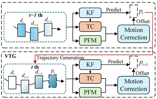
Figure 8.
Structure of virtual trajectory generation. The VTG module validates the target position predicted by KF using the temporal and physical similarity provided by TC and PFM.
For trajectories that remain inactive in frame , if no new updates are received in subsequent frame matching, their positions are predicted using Kalman filtering based on observations from the previous frame. These predicted positions are designated as “Virtual Detections”. The TC and PFM are utilized to assess the reliability of these virtual detections. The evaluation score is calculated as follows:
where are weighting coefficients. If no matching occurs in the frame t, the trajectory is further updated using virtual detection, named “Virtual Trajectory”. When a virtual detection score falls below a predefined threshold, corrections are implemented via optical flow and momentum m.
To mitigate error accumulation from prolonged virtual trajectory maintenance, a health score governs their validity. This score decays temporally to limit noise from over-prediction:
where represents the consecutive unmatched duration, and is the decay factor. Trajectories are terminated when drops below the deletion threshold, set to a value of 30 in this paper. The “Virtual Trajectory” relies on the KF motion model and is constrained through temporal–physical similarity metrics. Given its lower reliability, it is assigned a lower matching priority compared to real activated trajectories during the data association process to mitigate the risk.
2.6. Parameter Selection
Table 2 outlines the specifications of the training and testing environments, including processor configurations, GPU specifications, memory capacity, development environment, and other relevant technical parameters.
Table 2.
Training and testing environments.
For YOLOX detector [31] training, the input image dimensions are set to , and the batch size is set to 48. Training is conducted using the FireMOT dataset, which comprises 30,375 images, over a course of 300 epochs. Early termination is initiated if the validation metrics exhibit minimal fluctuation in the most recent 50 epochs. All other parameters conformed to the default configurations [31].
For the TC module of the tracker, historical trajectory sequences with a temporal length of five frames are extracted from the training dataset. Positive samples are defined as the target bounding box in the subsequent frame of each trajectory, while negative samples are taken from bounding boxes of different trajectories in the next frame. The ratio of positive to negative samples is kept at 6:4. To optimize the model, binary cross-entropy loss is utilized with a batch size of 2048 and the Adam optimizer. The initial learning rate is 0.0001, maintained over 300 epochs, with early stopping applied according to the validation stability criterion. During the tracking process, the parameters for the data association component of HAS remained consistent with [10]. AO-OCSORT identified key parameters for FireMOT through extensive experimentation, which included trajectory length, encoder depth, scene classification threshold , duplicate filtering threshold , and deletion criterion .
- (1)
- Selection of Trajectory Length
Table 3 illustrates the impact of trajectory length on tracking accuracy. Trajectories that are too short fail to capture comprehensive motion patterns, while excessively long trajectories introduce disruptive noise. The TC module achieves optimal performance with a trajectory length of 5, striking a balance between retaining localized details and representing broader temporal trends. At a length of 3, the performance slightly declines due to inadequate modeling of temporal trends. Conversely, extending trajectories beyond the optimal length results in a gradual drop in performance, mainly due to the accumulation of redundant noise.
Table 3.
Selection of trajectory length. The optimal value is indicated in boldface.
- (2)
- Selection of Encoder Depth
In the study of temporal information encoding for sequence modeling, we explored the effects of architectural modifications. As demonstrated in Table 4, the six-layer encoder configuration yielded optimal performance, whereas the three-layer variant suffered from inadequate hierarchical feature extraction and consequently exhibited poorer results. Conversely, the nine-layer architecture experienced performance saturation, possibly due to diminishing returns in deeper structures. The twelve-layer model overfitted to complex details in temporal patterns, leading to a decline in performance. Thus, our proposed framework integrates a six-layer encoder architecture, effectively balancing the capture of long-range dependencies with computational efficiency.
Table 4.
Selection of encoder depth. The optimal value is indicated in boldface.
- (3)
- Selection of Scene Classification Threshold
The scene classification threshold serves to assess the environmental context of trajectory data, thereby determining whether trajectories use IoU matching alone or incorporate multi-level matching involving the joint TC module, PFM, and IoU. Given that the introduction of the TC and PFM modules increases computational demands, this threshold critically affects the balance between model accuracy and inference speed. On the FireMOT dataset, a comprehensive analysis of this threshold is performed, evaluating tracking accuracy and speed at various thresholds. The experimental results are presented in Figure 9.
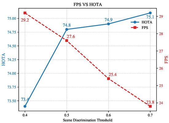
Figure 9.
Selection of scene classification threshold.
Figure 9 illustrates that increasing the scene classification threshold incrementally activates multi-level matching for a greater number of trajectories, thus improving association precision. However, this additional computational load decreases inference speed—while the higher-order tracking accuracy (HOTA) increases with higher thresholds, the FPS declines. A threshold of 0.5 was identified as optimal; raising it from 0.4 to 0.5 results in a negligible FPS reduction of 1.6 FPS yet yields a HOTA improvement of 1.4%. Beyond this threshold, HOTA growth slows down, although FPS continues to drop. Therefore, to optimize the balance between precision and speed, a threshold of 0.5 is chosen for the experiments in this study.
- (4)
- Selection of Duplicate Filtering Threshold
In the context of PFM, flame clusters may often be redundantly identified or inaccurately segmented due to motion blur and occlusion effects. To address this issue, the duplicate filtering threshold, , is utilized to filter out repetitive identifications. However, setting the threshold too low can inadvertently remove valid detection bounding boxes, leading to an increased rate of missed detections. Conversely, setting it too high may retain unnecessary duplicates, thereby increasing the occurrence of false positives. Therefore, selecting an optimal threshold is crucial for balancing the trade-off between false positives and missed detections. Experimental results demonstrating this balance are presented in Table 5. In scenarios such as forest fires, repeated detections can occur due to dynamic blur or occlusions. Lower thresholds tend to increase false negatives (FN), whereas higher thresholds elevate false positives (FP). At a threshold of 0.6, the model attains its best balance, achieving a 74.3% multiple object tracking accuracy (MOTA).
Table 5.
Selection of duplicate filtering threshold. The optimal value is indicated in boldface.
- (5)
- Selection of Dynamic Filtering Threshold
In forest fire scenarios, the rapid and intense variations of flames often lead detectors to produce low-confidence bounding boxes for large flame clusters, with multiple low-score detections redundantly anchoring the same target. To address this issue, we investigate the impact of different filtering thresholds on tracking performance. As shown in Figure 10, the fixed threshold for the blue line achieves an optimal performance of 74.2% at 0.6. The dynamic thresholds (orange line) with a base value of 0.5 and adaptive scaling based on a flame area achieve the best MOTA, effectively addressing redundant low-score detections in dynamic fire scenarios.
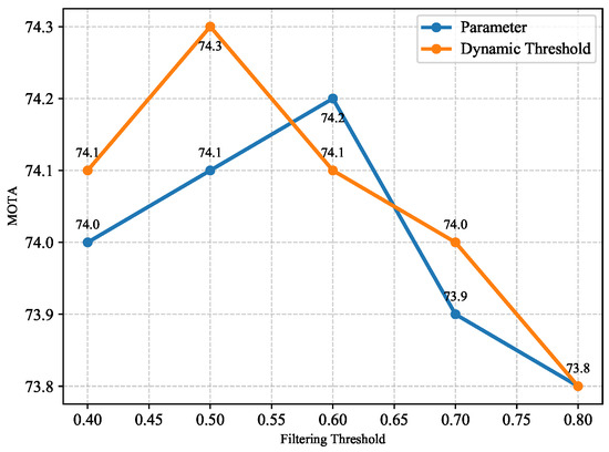
Figure 10.
Selection of dynamic filtering threshold.
3. Result and Discussion
3.1. Experimental Calculation and Result Analysis
To validate the accuracy of the proposed forest fire-tracking model, experiments are conducted using the FireMOT dataset. Additionally, to enhance the generalization capability of the proposed method in diverse scenarios, the VisDrone [12], MOT17 [13], and DanceTrack [14] datasets are included. The version incorporating temporal–physical similarity into the baseline OC-SORT method is referred to as TC-OCSORT, while the version that includes all components proposed in this paper is termed AO-OCSORT.
This paper uses higher-order tracking accuracy (HOTA) [37] as the primary evaluation metric. A significant advantage of HOTA is its balanced evaluation of detection confidence and cross-frame identity association continuity through a dual alignment strategy. Unlike the traditional multiple object tracking accuracy (MOTA) [38], which focuses on cumulative detection errors, HOTA separates detection and association errors, offering a more comprehensive assessment of tracking system performance. To further evaluate performance in complex scenarios, the identity F1 score (IDF1) [39] and MOTA are utilized, emphasizing identity preservation under challenges such as occlusion and deformation. Detection accuracy (DetA) [11] assesses the influence of detector performance, while association accuracy (AssA) [11] is introduced as a specialized benchmark for trajectory association. AssA isolates detection quality from association evaluation by determining optimal subspace mappings for cross-frame trajectory matching.
For the generalization datasets VisDrone [12], MOT17 [13], and DanceTrack [14], we adhered to the standard metric settings for comparison, as these datasets include publicly reported baseline methods. VisDrone utilizes metrics such as MOTA (multi-object tracking accuracy), IDF1 (ID F1 score), FP (false positives), FN (false negatives), and IDSW (identity switches). This community-standard practice ensures fair comparison with prior work on VisDrone [12]. Here, false positives are detections not corresponding to any ground-truth objects, whereas false negatives are ground-truth objects missed by the tracker. Identity switches measure the frequency of changes in the tracked identity of objects. IDSW counts the number of times a tracked object’s identity incorrectly switches to a different ground-truth identity between consecutive frames. This occurs when a tracker assigns a new ID to an object previously matched with another ID. Both MOT17 and DanceTrack employ evaluation settings consistent with those of FireMOT. To ensure unbiased performance evaluation, fire domain-specific processing modules are deactivated through model weight adjustments.
- (1)
- FireMOT Dataset
The dataset presents primary challenges involving complex nonlinear motion patterns and interference caused by overlapping targets. Experimental analysis indicates that OC-SORT, optimized specifically for addressing nonlinear motion challenges, delivers the highest performance among Kalman filtering-based methods. DiffMOT, utilizing a learning-based framework, excels in modeling nonlinear motion and is the nearest competitor to the proposed method. As shown in Table 6, our AO-OCSORT integrates temporal–physical similarity metrics and addresses detection gaps through virtual trajectory generation, significantly enhancing tracking robustness in forest fire scenarios. Compared to the baseline (OC-SORT), AO-OCSORT achieves improvements of 5.3% in HOTA, 11.3% in AssA, and 9.3% in IDF1. Furthermore, it surpasses the state-of-the-art DiffMOT by 2.3% in HOTA, demonstrating its enhanced effectiveness in forest fire-tracking applications.
Table 6.
Results on the FireMOT dataset. The optimal value is indicated in boldface.
Figure 11 illustrates a comparative analysis of tracking performance on the FireMOT dataset. In the first set of experiments, the flame located in the center of frame #659 and the adjacent flame are assigned identifiers 7 and 1, respectively. At the start of frame #660, these identifiers are lost due to rapid camera movement. However, by frame #662, the flames are tracked again, albeit with reassigned identifiers 35 and 34. Despite these changes, our methodology consistently preserved the identities of the flame targets throughout frames #659 to #662.
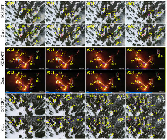
Figure 11.
Visualization of tracking results.
In the subsequent set of experiments, identity switching of tracked targets is observed between frames #293 and #296. The flame target initially identified as 1 in frame #293 is lost due to perspective jitter, but its identity is effectively reassigned in frame #296. The model proposed in this paper demonstrates stable tracking capabilities for flame targets across sequential images.
The third series of experiments examined the effects of rapid perspective shifts caused by drone movement. In frame #11, two flames located in the bottom left corner are assigned identities 2 and 4. Moving to frame #13, both flames experienced identity loss due to tracking drift. By frame #15, the trajectory originally labeled as 2 is reactivated and reassigned to a flame initially marked as 8, leading to an identity switch. Subsequently, in frame #17, the trajectory of flame 2 underwent another identity reassignment and was marked as 4, while its initial frame #11 identity was altered to #14.
The method analyzed in this paper robustly assigned identifiers 2 and 4 to the flames in the bottom left corner in frame #11, maintaining a stable track of flame 2 through frames #13, #15, and #17 without identity switching. After frame #11, flame 4, despite being momentarily obscured by vegetation, did not experience erroneous identity assignment. Furthermore, flame 8 was consistently tracked with minimal identity switching issues compared to OC-SORT.
- (2)
- VisDrone Dataset
The VisDrone dataset primarily consists of scenarios captured from UAV perspectives, where complex nonlinear motion is the main challenge. The proposed method employs temporal correlation analysis to model intricate motion dynamics and implements a hierarchical association strategy to balance missed detections and false alarms. Additionally, virtual trajectory generation addresses the fragmentation of trajectories caused by motion blur. As shown in Table 7, incorporating these enhancements improves AO-OCSORT by 1.8% in MOTA and 2.8% in IDF1 over the baseline. It is noteworthy that the more basic TC-OCSORT is also significantly superior to OC-SORT.
Table 7.
Results on the VisDrone dataset. The optimal value is indicated in boldface.
- (3)
- MOT17 Dataset
The MOT17 dataset is focused on analyzing pedestrian motion, where Kalman filter-based methods exhibit strong performance due to their natural compatibility with pedestrian motion patterns and the constant velocity model inherent to Kalman filtering. However, the proposed AO-OCSORT method surpasses the baseline model by 0.5% in HOTA, 1.7% in IDF1, and 0.9% in AssA on key evaluation metrics. As shown in Table 8, this improvement is attributed to the integration of TC and a HAS, which effectively addresses the challenges of partial occlusion in pedestrian tracking.
Table 8.
Results on the MOT17 dataset. The optimal value is indicated in boldface.
- (4)
- DanceTrack Dataset
The primary challenges of the DanceTrack dataset arise from significant deformations and intricate object interactions. Table 9 shows the tracking results of DanceTrack dataset. By utilizing the temporal correlation module’s enhanced capability to model nonlinear motion, the proposed AO-OCSORT exhibits superior performance, with improvements of 2.4% in HOTA, 3% in IDF1, and 2.4% in AssA compared to the baseline. Furthermore, it consistently outperforms the existing DiffMOT framework.
Table 9.
Results onthe DanceTrack dataset. The optimal value is indicated in boldface.
3.2. The Effect of Different Modules on Tracking
Table 10 illustrates the impact of various modules on similarity metric computation: the temporal correlation (TC) module, physical feature modeling (PFM) module, hierarchical association strategy (HAS), and virtual trajectory generation (VTG) module. Introducing the TC module alone resulted in a 3.5% enhancement in HOTA, highlighting its efficacy in modeling long-term temporal dependencies. Both IDF1 and AssA metrics increased by 5.7% and 6.8%, respectively, further validating the module’s ability to improve tracking consistency. The PFM module boosted IDF1 by 1.1%, emphasizing its utility in accurately distinguishing flame target identities. Implementing HAS led to increases in HOTA and AssA of 0.6% and 1.3%, respectively, demonstrating its adaptability to dynamic fire scenarios. Finally, the integration of the VTG module increased AssA by 0.8%, substantiating its effectiveness in addressing detection gaps through trajectory extrapolation.
Table 10.
Impact of AO-OCSORT modules on model performance. The optimal value is indicated in boldface.
As the model progresses from YOLOX-s to YOLOX-x, the increase in parameter count leads to enhanced detection performance, which subsequently improves tracking accuracy. However, this improvement comes with a significant decrease in inference speed. As shown in Table 11, the trade-off between accuracy and computational efficiency requires careful evaluation. To balance these competing priorities, this study utilizes YOLOX-l as the detector, achieving a frame rate of 28.1 FPS, thus enabling real-time tracking performance.
Table 11.
Impact of detector scale on model performance. The optimal value is indicated in boldface.
3.3. Discussion
The proposed AO-OCSORT exhibits superior performance on the FireMOT dataset, surpassing the baseline OC-SORT by 5.3% in HOTA and outperforming the leading competitor, DiffMOT, by 2.3% in HOTA. It consistently demonstrates generalizability across various scenarios, including VisDrone (MOTA increase of 1.8%), MOT17 (HOTA increase of 0.5%), and DanceTrack (HOTA increase of 2.4%). This advancement is chiefly attributed to the synergistic integration of three distinct modules. The TC module, capable of simulating complex nonlinear motion patterns, accounts for 81% of the total HOTA gain and addresses unstable flame trajectory propagation in UAV fire scenarios. Furthermore, the physical features introduced by the PFM significantly enhance MOTA. The temporal–physical similarity metric works in conjunction with HAS and VTG to further mitigate occlusion, as evidenced by substantial reductions in both false positives (FP) and false negatives (FN) on the VisDrone dataset.
Crucially, while the PFM module bolsters fire-specific discrimination using flame texture descriptors (resulting in a 9.3% increase in FireMOT IDF1), its dependence on optical features renders it susceptible to environmental interference, notably in differentiating smoke plumes from low-intensity flames. Despite achieving a balanced accuracy and processing speed (28.1 FPS with the YOLOX-l detector), the model is hindered by detector degradation under extreme conditions. Future research should focus on developing adaptive multi-spectral PFM features that integrate infrared and visible-light data, effectively resolving smoke-related ambiguities. Additionally, computational enhancements for edge deployment should be pursued to enable real-time wildfire monitoring on aerial platforms.
4. Conclusions
To address the critical limitations in drone-based forest fire tracking, especially concerning flame motion patterns viewed from a dynamic perspective, non-rigid target features, and trajectory fragmentation due to motion blur and environmental interference, existing solutions often fall short in accurately modeling the unique temporal dynamics and physical characteristics of flames. This study proposes AO-OCSORT, a redesigned multi-target tracking system for fire scenes. This method incorporates temporal–physical similarity metrics into the data association process to tackle issues related to flame dynamics and characteristics. An encoder–decoder framework with a Mamba structure models temporal tracking information as target trajectory similarity metrics, while a specialized physical feature modeling module captures flame-specific attributes. Together, these form a joint temporal–physical similarity metrics representation to enhance robustness. A hierarchical association strategy dynamically allocates matching resources based on scene complexity and conducts detection filtering, addressing the balance between accuracy and efficiency. To minimize trajectory fragmentation, a virtual trajectory generation module uses a kinematic interpolation approach with dual-verification. Extensive experiments conducted on FireRemote demonstrate that the proposed method surpasses advanced trackers. Validation on VisDrone, MOT17, and DanceTrack further supports its generalization capabilities. By explicitly tackling flame-specific challenges neglected by general trackers, this study lays a critical foundation for accurate fire spread prediction and optimized firefighting strategies. However, considering that the physical feature modeling used for fire object characteristics focuses solely on flame features, it might prove inadequate when faced with smoke and certain extreme conditions. Future work aims to integrate multimodal information to address this limitation and to consider deployment efficiency on embedded platforms more fully.
Author Contributions
Conceptualization, D.Y. and X.X.; methodology, X.X.; software, X.X.; validation, G.N. and X.W.; resources, D.Y.; data curation, X.X.; writing—original draft preparation, G.N.; writing—review and editing, G.N.; visualization, D.Z. All authors have read and agreed to the published version of the manuscript.
Funding
This research was funded by the following grants: Primary Research & Development Plan of Heilongjiang Province (Grant No. GA23A903), Vessel and Offshore Platform Safety Management Simulation Training System Development (Grant No. 2024ZX03B01), Aeronautical Science Foundation of China (Grant No. 202400550P6001), and Fundamental Research Funds for the Central Universities in China (Grant No. 3072024XX0602).
Data Availability Statement
The original contributions presented in this study are included in the article. Further inquiries can be directed to the corresponding authors.
Conflicts of Interest
The authors declare no conflicts of interest.
References
- Baldrian, P.; López-Mondéjar, R.; Kohout, P. Forest microbiome and global change. Nat. Rev. Microbiol. 2023, 21, 487–501. [Google Scholar] [CrossRef] [PubMed]
- Kinaneva, D.; Hristov, G.; Raychev, J.; Zahariev, P. Early forest fire detection using drones and artificial intelligence. In Proceedings of the 2019 42nd International Convention on Information and Communication Technology, Electronics and Microelectronics (MIPRO), Opatija, Croatia, 20–24 May 2019; IEEE: Piscataway, NJ, USA, 2019; pp. 1060–1065. [Google Scholar]
- Dogra, R.; Rani, S.; Sharma, B. A review to forest fires and its detection techniques using wireless sensor network. In Advances in Communication and Computational Technology: Select Proceedings of ICACCT 2019; Springer: Berlin/Heidelberg, Germany, 2021; pp. 1339–1350. [Google Scholar]
- Amosa, T.I.; Sebastian, P.; Izhar, L.I.; Ibrahim, O.; Ayinla, L.S.; Bahashwan, A.A.; Bala, A.; Samaila, Y.A. Multi-camera multi-object tracking: A review of current trends and future advances. Neurocomputing 2023, 552, 126558. [Google Scholar] [CrossRef]
- Lv, W.; Huang, Y.; Zhang, N.; Lin, R.S.; Han, M.; Zeng, D. Diffmot: A real-time diffusion-based multiple object tracker with non-linear prediction. In Proceedings of the IEEE/CVF Conference on Computer Vision and Pattern Recognition, Seattle, WA, USA, 16–22 June 2024; pp. 19321–19330. [Google Scholar]
- Du, Y.; Zhao, Z.; Song, Y.; Zhao, Y.; Su, F.; Gong, T.; Meng, H. Strongsort: Make deepsort great again. IEEE Trans. Multimed. 2023, 25, 8725–8737. [Google Scholar] [CrossRef]
- Gao, X.; Wang, Z.; Wang, X.; Zhang, S.; Zhuang, S.; Wang, H. DetTrack: An algorithm for multiple object tracking by improving occlusion object detection. Electronics 2023, 13, 91. [Google Scholar] [CrossRef]
- Gao, R.; Wang, L. MeMOTR: Long-term memory-augmented transformer for multi-object tracking. In Proceedings of the IEEE/CVF International Conference on Computer Vision, Paris, France, 1–6 October 2023; pp. 9901–9910. [Google Scholar]
- Veeramani, B.; Raymond, J.W.; Chanda, P. DeepSort: Deep convolutional networks for sorting haploid maize seeds. BMC Bioinform. 2018, 19, 289. [Google Scholar] [CrossRef] [PubMed]
- Zhang, Y.; Sun, P.; Jiang, Y.; Yu, D.; Weng, F.; Yuan, Z.; Luo, P.; Liu, W.; Wang, X. Bytetrack: Multi-object tracking by associating every detection box. In Proceedings of the European Conference on Computer Vision, Tel Aviv, Israel, 23–27 October 2022; Springer: Berlin/Heidelberg, Germany, 2022; pp. 1–21. [Google Scholar]
- Cao, J.; Pang, J.; Weng, X.; Khirodkar, R.; Kitani, K. Observation-centric sort: Rethinking sort for robust multi-object tracking. In Proceedings of the IEEE/CVF Conference on Computer Vision and Pattern Recognition, Vancouver, BC, Canada, 17–24 June 2023; pp. 9686–9696. [Google Scholar]
- Zhu, P.; Wen, L.; Du, D.; Bian, X.; Fan, H.; Hu, Q.; Ling, H. Detection and tracking meet drones challenge. IEEE Trans. Pattern Anal. Mach. Intell. 2021, 44, 7380–7399. [Google Scholar] [CrossRef]
- Milan, A.; Leal-Taixé, L.; Reid, I.; Roth, S.; Schindler, K. MOT16: A benchmark for multi-object tracking. arXiv 2016, arXiv:1603.00831. [Google Scholar]
- Sun, P.; Cao, J.; Jiang, Y.; Yuan, Z.; Bai, S.; Kitani, K.; Luo, P. Dancetrack: Multi-object tracking in uniform appearance and diverse motion. In Proceedings of the IEEE/CVF Conference on Computer Vision and Pattern Recognition, New Orleans, LA, USA, 18–24 June 2022; pp. 20993–21002. [Google Scholar]
- Kalman, R.E. A new approach to linear filtering and prediction problems. J. Basic Eng. 1960, 82, 35–45. [Google Scholar] [CrossRef]
- Bewley, A.; Ge, Z.; Ott, L.; Ramos, F.; Upcroft, B. Simple online and realtime tracking. In Proceedings of the 2016 IEEE International Conference on Image Processing (ICIP), Phoenix, AZ, USA, 25–28 September 2016; IEEE: Piscataway, NJ, USA, 2016; pp. 3464–3468. [Google Scholar]
- Aharon, N.; Orfaig, R.; Bobrovsky, B.Z. Bot-sort: Robust associations multi-pedestrian tracking. arXiv 2022, arXiv:2206.14651. [Google Scholar]
- Xie, M.; Wu, J.; Zhang, L.; Li, C. A novel boiler flame image segmentation and tracking algorithm based on YCbCr color space. In Proceedings of the 2009 International Conference on Information and Automation, Zhuhai, Macau, 22–24 June 2009; IEEE: Piscataway, NJ, USA, 2009; pp. 138–143. [Google Scholar]
- Khalil, A.; Rahman, S.U.; Alam, F.; Ahmad, I.; Khalil, I. Fire detection using multi color space and background modeling. Fire Technol. 2021, 57, 1221–1239. [Google Scholar] [CrossRef]
- Rong, J.; Zhou, D.; Yao, W.; Gao, W.; Chen, J.; Wang, J. Fire flame detection based on GICA and target tracking. Opt. Laser Technol. 2013, 47, 283–291. [Google Scholar] [CrossRef]
- Yuan, C.; Liu, Z.; Zhang, Y. UAV-based forest fire detection and tracking using image processing techniques. In Proceedings of the 2015 International Conference on Unmanned Aircraft Systems (ICUAS), Denver, CO, USA, 9–12 June 2015; IEEE: Piscataway, NJ, USA, 2015; pp. 639–643. [Google Scholar]
- Daoud, Z.; Ben Hamida, A.; Ben Amar, C. Fire object detection and tracking based on deep learning model and Kalman Filter. Arab. J. Sci. Eng. 2024, 49, 3651–3669. [Google Scholar] [CrossRef]
- Redmon, J.; Farhadi, A. Yolov3: An incremental improvement. arXiv 2018, arXiv:1804.02767. [Google Scholar]
- Yuan, C.; Liu, Z.; Zhang, Y. Fire detection using infrared images for UAV-based forest fire surveillance. In Proceedings of the 2017 International Conference on Unmanned Aircraft Systems (ICUAS), Miami, FL, USA, 13–16 June 2017; IEEE: Piscataway, NJ, USA, 2017; pp. 567–572. [Google Scholar]
- Cai, B.; Xiong, L.; Zhao, J. Forest fire visual tracking with mean shift method and gaussian mixture model. In Smart Innovations in Communication and Computational Sciences: Proceedings of ICSICCS 2017; Springer: Berlin/Heidelberg, Germany, 2019; Volume 2, pp. 329–337. [Google Scholar]
- Mouelhi, A.; Bouchouicha, M.; Sayadi, M.; Moreau, E. Fire tracking in video sequences using geometric active contours controlled by artificial neural network. In Proceedings of the 2020 4th International Conference on Advanced Systems and Emergent Technologies (IC_ASET), Hammamet, Tunisia, 15–18 December 2020; IEEE: Piscataway, NJ, USA, 2020; pp. 338–343. [Google Scholar]
- De Venâncio, P.V.A.; Rezende, T.M.; Lisboa, A.C.; Barbosa, A.V. Fire detection based on a two-dimensional convolutional neural network and temporal analysis. In Proceedings of the 2021 IEEE Latin American Conference on Computational Intelligence (LA-CCI), Temuco, Chile, 2–4 November 2021; pp. 1–6. [Google Scholar]
- Bochkovskiy, A.; Wang, C.Y.; Liao, H.Y.M. Yolov4: Optimal speed and accuracy of object detection. arXiv 2020, arXiv:2004.10934. [Google Scholar]
- Gu, A.; Goel, K.; Ré, C. Efficiently modeling long sequences with structured state spaces. arXiv 2021, arXiv:2111.00396. [Google Scholar]
- Gu, A.; Dao, T. Mamba: Linear-time sequence modeling with selective state spaces. arXiv 2023, arXiv:2312.00752. [Google Scholar]
- Ge, Z.; Liu, S.; Wang, F.; Li, Z.; Sun, J. Yolox: Exceeding yolo series in 2021. arXiv 2021, arXiv:2107.08430. [Google Scholar]
- Girshick, R.; Donahue, J.; Darrell, T.; Malik, J. Rich feature hierarchies for accurate object detection and semantic segmentation. In Proceedings of the IEEE Conference on Computer Vision and Pattern Recognition, Columbus, Ohio, USA, 23–28 June 2014; pp. 580–587. [Google Scholar]
- Vaswani, A.; Shazeer, N.; Parmar, N.; Uszkoreit, J.; Jones, L.; Gomez, A.N.; Kaiser, Ł.; Polosukhin, I. Attention is all you need. In Advances in Neural Information Processing Systems; MIT Press: Long Beach, California, USA, 2017; Volume 30. [Google Scholar]
- Dosovitskiy, A.; Beyer, L.; Kolesnikov, A.; Weissenborn, D.; Zhai, X.; Unterthiner, T.; Dehghani, M.; Minderer, M.; Heigold, G.; Gelly, S.; et al. An image is worth 16x16 words: Transformers for image recognition at scale. arXiv 2020, arXiv:2010.11929. [Google Scholar]
- Hu, B.; Luo, R.; Liu, Z.; Wang, C.; Liu, W. TrackSSM: A General Motion Predictor by State-Space Model. arXiv 2024, arXiv:2409.00487. [Google Scholar]
- Cho, K.; Van Merriënboer, B.; Gulcehre, C.; Bahdanau, D.; Bougares, F.; Schwenk, H.; Bengio, Y. Learning phrase representations using RNN encoder-decoder for statistical machine translation. arXiv 2014, arXiv:1406.1078. [Google Scholar]
- Luiten, J.; Osep, A.; Dendorfer, P.; Torr, P.; Geiger, A.; Leal-Taixé, L.; Leibe, B. Hota: A higher order metric for evaluating multi-object tracking. Int. J. Comput. Vis. 2021, 129, 548–578. [Google Scholar] [CrossRef] [PubMed]
- Bernardin, K.; Stiefelhagen, R. Evaluating multiple object tracking performance: The clear mot metrics. EURASIP J. Image Video Process. 2008, 2008, 246309. [Google Scholar] [CrossRef]
- Ristani, E.; Solera, F.; Zou, R.; Cucchiara, R.; Tomasi, C. Performance measures and a data set for multi-target, multi-camera tracking. In Proceedings of the European Conference on Computer Vision, Amsterdam, The Netherlands, 8–10, 15–16 October 2016; Springer: Cham, Switzerland, 2016; pp. 17–35. [Google Scholar]
- Zhang, Y.; Wang, C.; Wang, X.; Zeng, W.; Liu, W. Fairmot: On the fairness of detection and re-identification in multiple object tracking. Int. J. Comput. Vis. 2021, 129, 3069–3087. [Google Scholar] [CrossRef]
- Zeng, F.; Dong, B.; Zhang, Y.; Wang, T.; Zhang, X.; Wei, Y. Motr: End-to-end multiple-object tracking with transformer. In Proceedings of the European Conference on Computer Vision, Tel Aviv, Israel, 23–27 October 2022; Springer: Cham, Switzerland, 2022; pp. 659–675. [Google Scholar]
- Liu, S.; Li, X.; Lu, H.; He, Y. Multi-object tracking meets moving UAV. In Proceedings of the IEEE/CVF Conference on Computer Vision and Pattern Recognition, New Orleans, LA, USA, 18–24 June 2022; pp. 8876–8885. [Google Scholar]
- Wu, H.; Nie, J.; He, Z.; Zhu, Z.; Gao, M. One-shot multiple object tracking in UAV videos using task-specific fine-grained features. Remote. Sens. 2022, 14, 3853. [Google Scholar] [CrossRef]
- Zhou, X.; Koltun, V.; Krähenbühl, P. Tracking objects as points. In Proceedings of the European Conference on Computer Vision, Glasgow, UK, 23–28 August 2020; Springer: Cham, Switzerland, 2020; pp. 474–490. [Google Scholar]
- Meinhardt, T.; Kirillov, A.; Leal-Taixe, L.; Feichtenhofer, C. Trackformer: Multi-object tracking with transformers. In Proceedings of the IEEE/CVF Conference on Computer Vision and Pattern Recognition, New Orleans, LA, USA, 18–24 June 2022; pp. 8844–8854. [Google Scholar]
Disclaimer/Publisher’s Note: The statements, opinions and data contained in all publications are solely those of the individual author(s) and contributor(s) and not of MDPI and/or the editor(s). MDPI and/or the editor(s) disclaim responsibility for any injury to people or property resulting from any ideas, methods, instructions or products referred to in the content. |
© 2025 by the authors. Licensee MDPI, Basel, Switzerland. This article is an open access article distributed under the terms and conditions of the Creative Commons Attribution (CC BY) license (https://creativecommons.org/licenses/by/4.0/).