Comparison Between Traditional Forest Inventory and Remote Sensing with Random Forest for Estimating the Periodic Annual Increment in a Dry Tropical Forest

Abstract

This study evaluates the effectiveness of combining remote sensing techniques with the Random Forest algorithm for estimating the Periodic Annual Increment (PAI) in a dry tropical forest located within the Caatinga biome in northeastern Brazil. The analysis integrates forest inventory data collected from permanent plots monitored between 2011 and 2019 with Landsat satellite imagery processed through the Google Earth Engine platform. By incorporating surface reflectance and vegetation indices, the approach significantly improved the accuracy of productivity estimates while reducing the costs and efforts associated with traditional field-based methods. The Random Forest model achieved a strong performance (R² = 0.8867; RMSE = 0.87), and its predictions were further refined using post-processing correction factors. These results demonstrate the potential of data-driven modeling to support forest monitoring and sustainable management practices, especially in ecosystems vulnerable to the impacts of climate change.

1. Introduction

Native forests play a central role in the provision of timber and non-timber products, such as wood, fibers, and fuels. Beyond their industrial utility, these resources are renewable and exhibit high energy efficiency, making them environmentally responsible alternatives to fossil fuel-derived products, plastics, and metals. When sustainable management techniques are adopted, these forests contribute to soil and water conservation [1], the recovery of degraded areas [2], and offer social benefits, including job creation and regional development [3].

Research on dry tropical forests in Brazil has investigated aspects related to forest recovery [4], structure and dynamics [5,6], carbon stock [7,8,9], and, more recently, the use of remote sensing for vegetation monitoring [10,11]. These efforts aim to bridge knowledge gaps regarding the ecology of these forests, particularly in the context of climate change [12], which exacerbates their vulnerability due to the increasing frequency of extreme climatic events [13,14].

Although tropical forests are recognized for their high biodiversity, they may be dominated by a few species at local scales. This phenomenon is also observed in seasonally dry biomes, such as the Caatinga, where sparse vegetation can exhibit high diversity due to environmental heterogeneity and species’ adaptive strategies to extreme climatic conditions. Studies indicate that despite being predominantly xerophytic and of low density, the Caatinga harbors significant biodiversity, with structural variations influenced by climatic and edaphic factors [15,16]. Such dominance patterns often reflect successional and demographic variations over time [17]. Climatic factors, such as precipitation and temperature [18,19], along with soil fertility and other edaphic conditions [20,21], shape the structure and composition of these plant communities. Furthermore, species’ resilience to environmental disturbances is crucial for their survival and dispersal [22].

To better understand forest dynamics, growth assessment through the Periodic Annual Increment (PAI) has emerged as a critical metric. This measure allows for the evaluation of forest growth in response to environmental conditions. In dry tropical forests, such as the Caatinga, seasonal water availability plays a central role in influencing growth processes and natural regeneration. Extreme climatic events, such as severe droughts, can substantially alter forest dynamics, highlighting the need for studies correlating PAI with these environmental variables [23,24]. It is also crucial to further investigate the Cerrado and Caatinga biomes, considering anthropogenic impacts [25].

Traditionally, PAI monitoring has been conducted through permanent plots, where periodic measurements provide data on vegetation development. However, this method presents significant challenges, including the need for extensive fieldwork, high costs, and logistical difficulties in remote areas. These limitations can restrict the spatial and temporal scope of studies, compromising the effectiveness of continuous monitoring [26]. There is evidence of an encroachment process occurring in the Cerrado biome [27,28], which may also be taking place in the Caatinga. To understand such phenomena, methods with broad spatial and temporal coverage are essential.

With the advancement of remote sensing technologies, it has become possible to overcome some of these barriers. The use of satellite imagery and unmanned aerial vehicles (UAVs) allows for large-scale data collection with higher frequency and lower cost. One of the main applications of these technologies is the use of vegetation indices (VIs) and spectral reflectance, which are metrics derived from vegetation reflectance that enable the monitoring of vegetation cover, plant vigor, and ecosystem processes over time [29,30,31,32,33]. For example, Ref. [34] developed a low-cost UAV-based forest restoration monitoring protocol, demonstrating its effectiveness in Brazil’s Atlantic Forest. Similarly, Ref. [35] implemented a national-scale forest monitoring system in Tanzania using remote sensing data to support management and conservation decisions. These examples illustrate how remote sensing can complement traditional methods, providing a more comprehensive and updated view of forest dynamics.

Landsat satellite imagery has proven to be a valuable tool for multi-temporal analysis, enabling high-precision vegetation cover change detection over more than four decades [36,37,38,39], including harmonized data products [40,41]. The availability of orbital data and the demands associated with dry tropical forest monitoring require robust information extraction methods.

Machine learning algorithms, such as Random Forest, Gradient Boosting, Support Vector Machines (SVMs), and Artificial Neural Networks (ANNs), can enhance predictive capabilities and the analysis of complex ecosystems [42,43,44,45,46]. These algorithms, by handling large volumes of multivariate data, have demonstrated efficiency in ecological modeling, enabling the identification of relevant patterns and key variables influencing forest growth and species resilience [47,48,49].

Among these, Random Forest stands out for its robustness in analyzing large-scale multivariate datasets. This algorithm employs multiple decision trees to construct highly accurate predictive models, facilitating the identification of key factors affecting forest growth [42,50,51]. Its application in ecological studies provides valuable insights into the factors influencing forest dynamics and species resilience [50,52,53].

To assess the potential of machine learning techniques and satellite imagery, this study aims to compare the Periodic Annual Increment (PAI) estimates obtained through traditional field-based forest inventory methods with those derived from remote sensing techniques, employing machine learning algorithms such as Random Forest. The Caatinga biome was selected as the study area.

2. Materials and Methods

To provide a clear overview of the research workflow, Figure 1 presents a schematic representation of the methodological steps adopted in this study, highlighting the integration of field and orbital data, variable processing, statistical analysis, and the use of the Random Forest algorithm for the estimation and spatialization of the Periodic Annual Increment (PAI).

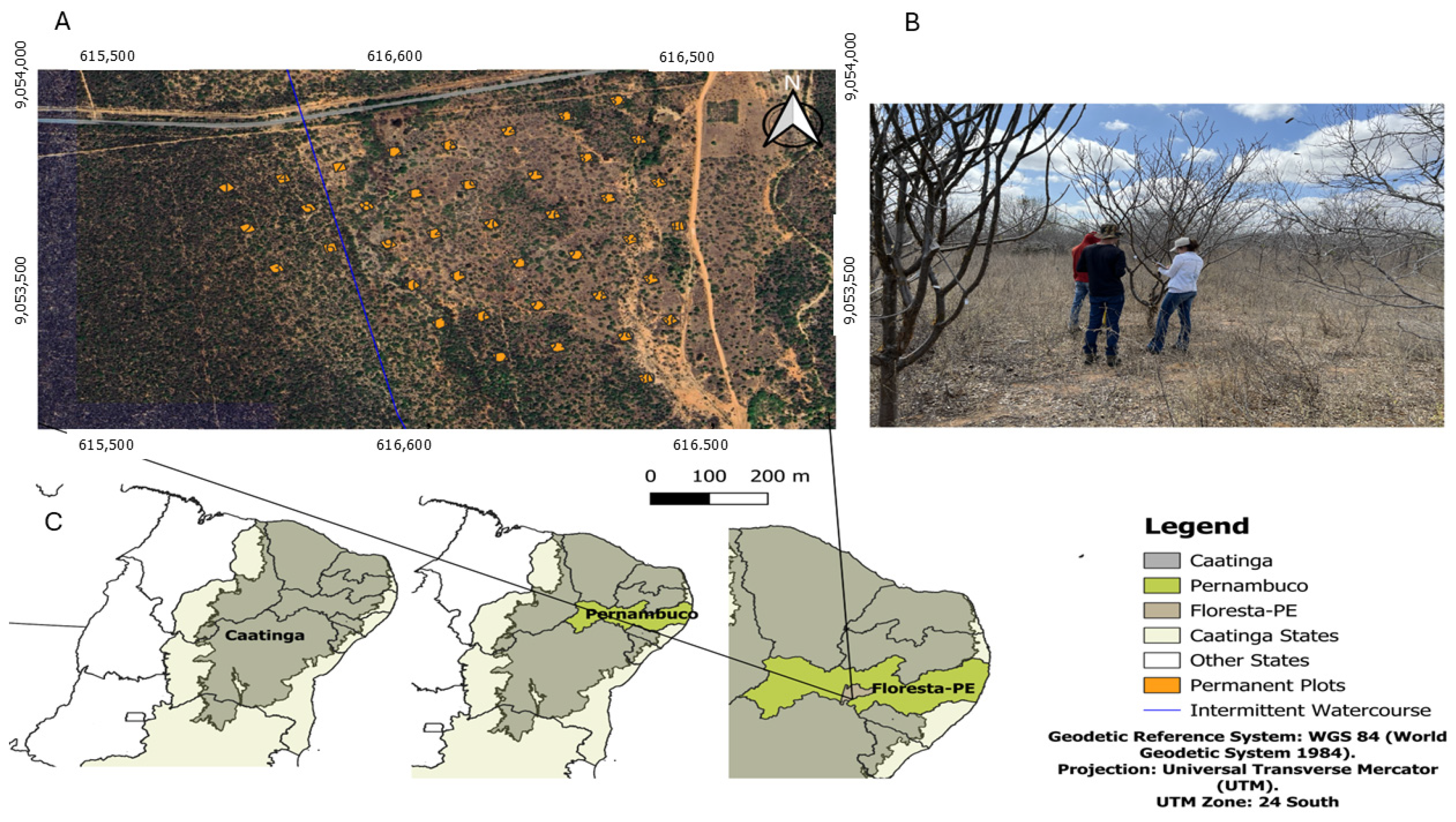
2.1. Study Area Location

The data were collected from a 1.6-hectare sampling area, located within Fazenda Itapemirim (Agrimex S.A, Floresta, Pernambuco, Brazil). The farm covers 5695.65 hectares, where native vegetation was cleared in 1987 using tractors and chains [54]. At the time, the purpose of removing the native vegetation was to establish exotic species. However, the project failed, leading to the abandonment of the area, which subsequently entered a natural regeneration process.

The study area has been monitored since 2008 through 40 permanent plots, each measuring 20 m × 20 m (400 m²), totaling a sampled area of 1.6 ha. The plots are evenly spaced 80 m apart, measured from the center, and the buffer zone between plots is 60 m (Figure 2).

2.2. Field Data Collection

For standardization purposes, plants were identified and tagged at a height of 1.30 m above ground. Annually, starting in 2011, all shrub and tree species were identified and measured in each sampling unit, recording the circumference at 1.30 m above ground level (C ≥ 6 cm) and total height (H). Additionally, newly recruited individuals (plants and/or stems reaching the minimum C criterion), as well as dead and fallen individuals, were recorded. This study followed the nomenclature and measurement standards for forest inventory [55].

A plant was considered any part belonging to a single-root system, based on the observation of its above ground structure. In cases where bifurcations occurred below 1.30 m in the same plant and met the minimum inclusion criteria, they were recorded as stems.

Data were collected each September to coincide with the dry season. Circumference measurements were taken using a measuring tape, while height was measured with a graduated ruler, both with centimeter precision. Circumferences were converted to diameter at 1.30 m above ground level (D) by dividing C by π.

2.3. Climatic Data

Temperature and precipitation data for the period from 2009 to 2023 were obtained from the LP DAAC database (USGS, Sioux Falls, SD, USA) and from the Climate Hazards Center (University of California, Santa Barbara, CA, USA). The datasets used were the MODIS/006/MOD11A1 and CHIRPS/DAILY products, based on the geographic coordinates of the study area [56,57].

2.4. Remote Sensing Data

Landsat 5 and Landsat 8 satellite images (USGS, Sioux Falls, SD, USA) were selected from the complete collection available on the Google Earth Engine platform, using the LANDSAT/LT05/C02/T1_L2 and LANDSAT/LC08/C02/T1_L2 libraries, respectively. Landsat 5 was used for the year 2011, while Landsat 8 data were employed for the years 2013, 2015, 2017, and 2019.

The images were preprocessed by applying cloud and radiometric saturation masks, limiting cloud coverage to less than 60% to ensure data quality. After preprocessing, the spectral surface reflectance bands were corrected for each sensor, and vegetation indices were calculated for each analyzed year. These data were extracted specifically for the study area, ensuring temporal and spatial consistency and comparability (

Table 1. Vegetation indices used in the study area.

Vegetation Index	Formula	Reference Source
Normalized Difference Vegetation Index (NDVI)	(NIR − RED)/(NIR + RED)	[58]
Enhanced Vegetation Index (EVI)	2.5 × (NIR − RED)/(NIR + 6 × RED − 7.5 × BLUE + 1)	[59]
Soil-Adjusted Vegetation Index (SAVI)	(1 + L) × (NIR − RED)/(NIR + RED + L)	[60]
Green Normalized Difference Vegetation Index (GNDVI)	(NIR − GREEN)/(NIR + GREEN)	[61]
Normalized Difference Water Index (NDWI)	(NIR − SWIR)/(NIR + SWIR) or (GREEN − NIR)/(GREEN + NIR)	[62]
Normalized Difference Built-up Index (NDBI)	(SWIR − NIR)/(SWIR + NIR)	[63]
Moisture Stress Index (MSI)	SWIR/NIR	[64]
Normalized Burn Ratio (NBR)	(NIR − SWIR)/(NIR + SWIR)	[65]
Normalized Difference Snow Index (NDSI)	(GREEN − SWIR)/(GREEN + SWIR)	[66]
Leaf Area Index (LAI)	Ln((0.69 − SAVI)/0.59)/0.91	[67]

In which: NIR: Near-Infrared; RED: Red; GREEN: Green; BLUE: Blue; SWIR: Short-Wave Infrared; L: Soil adjustment factor for SAVI, which typically ranges from 0 (for dense vegetation cover) to 1 (for sparse vegetation cover); in this study, a value of 0.5 was used.

).

To ensure compatibility between the two sensors, Band 6 of the Landsat 5/TM satellite and Bands 1, 8, 9, 10 and 11 of the Landsat 8/OLI satellite were excluded from the analysis.

2.5. Recruitment and Mortality Dynamics

In this study, a two-year monitoring period was considered between surveys conducted from 2011 to 2019. Thus, an individual (stem) was classified as a recruit if it reached C ≥ 6 cm only in the second measurement. This means that individuals (stems) that emerged in 2013 were counted for the 2011–2013 interval, those that emerged in 2015 for the 2013–2015 interval, those that appeared in 2017 for the 2015–2017 interval, and those that appeared in 2019 for the 2017–2019 interval.

The recruitment rate was calculated using Equation (1).

$$\mathbf{T}\mathbf{R}=\left[\mathbf{1}-{\left(\mathbf{1}-{\displaystyle \frac{{\mathbf{N}}_{\mathbf{r}}}{{\mathbf{N}}_{\mathbf{f}}}}\right)}^{{\displaystyle \frac{\mathbf{1}}{\mathbf{t}}}}\right]\times \mathbf{100}$$

(1)

where: TR = recruitment rate (%); t = time elapsed between inventories (years); Nf = final count of living trees (stems) per hectare; Nr = number of recruited individuals (stems) per hectare.

For mortality estimation, an individual (stem) was considered dead if it was an adult shrub or tree with C ≥ 6 cm in the 2011 survey but was found dead in the subsequent 2013 survey (first interval: 2011–2013). For the second interval (2013–2015), trees recorded as alive in 2013 but dead in 2015 were counted. Similarly, for the third interval (2015–2017), trees that were alive in 2015 but dead in 2017 were considered. Finally, for the fourth interval (2017–2019), trees recorded as alive in 2017 but dead in 2019 were included in the mortality count.

The mortality rate was calculated using Equation (2).

$$\mathrm{T}\mathrm{M}=\left[1-{\left(1-{\displaystyle \frac{{\mathrm{N}}_{\mathrm{m}}}{{\mathrm{N}}_0}}\right)}^{{\displaystyle \frac{1}{\mathrm{t}}}}\right]\times 100$$

(2)

where: TM = mortality rate (%); t = time elapsed between inventories (years); N₀ = initial number of trees (stems) per hectare; Nm = number of dead individuals (stems) per hectare.

Growth estimates were obtained using the methodology proposed by [52], and the Periodic Annual Increments (PAIs) for field data were calculated based on the ratio between gross and net growth (including and excluding recruits, respectively) and the interval between measurement periods, according to Equations (3)–(6).

Cb_i = G₂ + M + MF + C + CF − G₁

(3)

Cb = G₂ + M + MF + C + CF − GI − GF − G₁

(4)

Cl_I = Cb_{i −} M + MF − G₁

(5)

Cl = G_{2 −} GI + GF − G₁

(6)

where: Cbi represents the gross growth including recruits; Cb is the gross growth excluding recruits; ClI corresponds to the net growth including recruits; Cl is the net growth excluding recruits. G₂ is the basal area (m² ha⁻¹) in the final inventory, at the end of the growth period, while G₁ is the basal area (m² ha⁻¹) in the initial inventory, at the beginning of the growth period. M represents the basal area of individual mortality (m² ha⁻¹), and MF is the basal area of stem mortality in living individuals (m² ha⁻¹). C refers to the basal area of harvested individuals (recruits) in m² ha⁻¹, and CF is the basal area of harvested stems (recruits within individuals) in m² ha⁻¹. GI denotes the basal area of recruited individuals (m² ha⁻¹), and GF represents the basal area of recruited stems within individuals (m² ha⁻¹).

2.6. Periodic Annual Increments

The Periodic Annual Increments in basal area (PAIs, mm.ha⁻¹) were obtained by calculating the ratio between Cbi, Cb, ClI, and Cl, and the interval between measurement periods, considering both individuals and stems.

Based on the estimation of Cb, the mean annual periodic increment in diameter was calculated using Equation (7).

$${\overline{\mathrm{P}\mathrm{A}\mathrm{I}}}_{\mathrm{d}}={\displaystyle \frac{1}{\mathrm{n}.\mathrm{a}}}\sqrt{{\displaystyle \frac{40000.{\mathrm{C}}_{\mathrm{b}}}{\mathsf{\pi }}}}$$

(7)

where: PAI represents the mean Periodic Annual Increment in diameter (mm.ha⁻¹); Cb is the gross growth excluding recruits; n is the number of individuals; and a is the interval between measurement occasions (2 years).

2.7. Modeling with Random Forest

Digital image processing was performed using QGIS (version 3.10.4, QGIS Development Team, Hannover, Germany). The extraction of pixel reflectance values for the analyzed periods was carried out using the Point Sampling Tool plugin (version 0.5.1, Kraków, Poland), which allowed for the capture of reflectance values associated with the study area. The extracted data, including reflectance and vegetation indices, were organized into an Excel spreadsheet, containing detailed information such as plot identification, metric coordinates, basal areas, Periodic Annual Increments, reflectance values from Landsat 5 and Landsat 8 bands, and the vegetation indices calculated for each plot and analyzed period. These variables were later used as predictors in machine learning modeling.

To estimate the Periodic Annual Increment (PAI) using the remote sensing variables of the study area, the Random Forest technique was employed, implemented in the Scikit-learn (version 1.2.2) library in Python (version 3.10.12, Python Software Foundation, Wilmington, DE, USA) [68,69]. Random Forest is an ensemble learning algorithm based on the aggregation of multiple decision trees. Each tree is built from a bootstrap sample of the dataset, and the final prediction is obtained by averaging the outputs of individual trees. This approach reduces overfitting and improves generalization, making it particularly robust for modeling complex and nonlinear relationships, as often encountered in ecological and remote sensing data [42,50,51]. In addition to this library, Pandas (version 1.5.3, PyData Development Team, Austin, TX, USA) [70] was used for data analysis, Scipy.stats (version 1.10.1, SciPy Developers, Austin, TX, USA) [71] for computing Spearman’s correlation, Matplotlib.pyplot (version 3.7.1, Matplotlib Development Team, New York, NY, USA) [72] and Seaborn (version 0.12.2, Michael Waskom, Stanford, CA, USA) [73] for generating graphs, and Numpy (version 1.24.3, NumPy Developers, Austin, TX, USA) [74] for matrix calculations.

Each model was trained with 400 estimators (trees), balancing prediction accuracy and computational efficiency. This number was chosen based on preliminary testing with different values (ranging from 100 to 500), which showed that performance gains stabilized around 400 estimators. Thus, this value was selected as an optimal point to avoid unnecessary computational cost while ensuring model robustness. The data were split into 80% for training and 20% for validation, following common predictive modeling practices [75].

The selection of variables was guided by the significance of Spearman’s correlation [76] (Equation (8)).

$${\mathrm{r}}_{\mathrm{s}}=1-{\displaystyle \frac{6\sum {\mathrm{d}}_{\mathrm{i}}^2}{\mathrm{n}({\mathrm{n}}^2-1)}}$$

(8)

where d_i represents the difference between the ranks of each pair of observations, and n is the number of observations.

The model performance metrics included the Coefficient of Determination (R²) and the Root Mean Square Error (RMSE) (Equations (9) and (10), respectively) to assess prediction accuracy [77].

$${\mathrm{R}}^2=1-{\displaystyle \frac{{\sum }_{\mathrm{i}=1}^{\mathrm{n}}({\mathrm{y}}_{\mathrm{i}}-{\widehat{\mathrm{y}}}_{\mathrm{i}}{)}^2}{{\sum }_{\mathrm{i}=1}^{\mathrm{n}}({\mathrm{y}}_{\mathrm{i}}-\overline{\mathrm{y}}{)}^2}}$$

(9)

where n is the number of observations, y_i represents the observed values, ŷ_i represents the predicted values from the model, and ȳ is the mean of the observed values.

$$\mathrm{R}\mathrm{M}\mathrm{S}\mathrm{E}=\sqrt{{\displaystyle \frac{{\sum }_{\mathrm{i}=1}^{\mathrm{n}}({\mathrm{y}}_{\mathrm{i}}-{\widehat{\mathrm{y}}}_{\mathrm{i}}{)}^2}{\mathrm{n}}}}$$

(10)

where y_i is the observed value, ŷ_i is the predicted value from the model, and n is the number of observations.

2.8. Bias Correction of Estimates

Due to the observed bias in the Random Forest models, considering the complexity of the forest structure in a dry tropical forest, a correction factor was applied based on the Periodic Annual Increment (PAI).

The correction factor was obtained as follows:

(a)

Estimation difference calculation: First, the absolute difference between the actual values and the predicted values was calculated and stored in a new column in the spreadsheet. This was carried out to quantify the estimation error for each observation (Equation (11)).

$${∆}_{\mathrm{i}}=\left|{\mathrm{y}}_{\mathrm{i}}-{\widehat{\mathrm{y}}}_{\mathrm{i}}\right|$$

(11)

where y_i represents the actual observed value of observation i, and ŷ_i is the value predicted by the Random Forest model.

(b)

Data classification: Next, the actual data were classified into ranges using the Qcut function, which divides the data into quantiles. The data were segmented into six equally sized classes, with an additional unit added to each class to avoid zero-based indexing, resulting in classes numbered 1 to 6. These classes were stored in a new column (Equation (12)).

$${\mathrm{C}}_{\mathrm{i}}=\mathrm{Classe}\left(\mathrm{y}\mathrm{i}\right),{\mathrm{C}}_{\mathrm{i}} \mathsf{ϵ} \left\{1,2,\dots ,\mathrm{k}\right\}$$

(12)

where k = 6 is the number of classes.

(c)

Correction factor calculation: For each previously defined class, a mean correction factor was calculated based on the estimation difference. This was carried out by grouping the data by class and obtaining the mean difference for each group. These factors represent the average adjustment required for each value class, considering both basal area and the Periodic Annual Increment (Equation (13)).

$${\mathrm{F}}_{\mathrm{c}}={\displaystyle \frac{1}{\mathrm{n}\mathrm{C}}}{\sum }_{\mathrm{i}\mathsf{ϵ}\mathrm{C}}{∆}_{\mathrm{i}}$$

(13)

where nC is the number of observations in class C, and Δ_i represents the estimation difference for observation i in class C.

(d)

Application of the correction factor: The correction factor was then applied to adjust the original predictions. For each observation, the respective correction factor was added to the estimated value, resulting in a new column of corrected predictions (Equation (14)).

$${{\widehat{\mathrm{y}}}_{\mathrm{i}}}^{\mathrm{c}\mathrm{o}\mathrm{r}\mathrm{r}}={\widehat{\mathrm{y}}}_{\mathrm{i}}+\mathrm{F}{\mathrm{C}}_{\mathrm{i}}$$

(14)

(e)

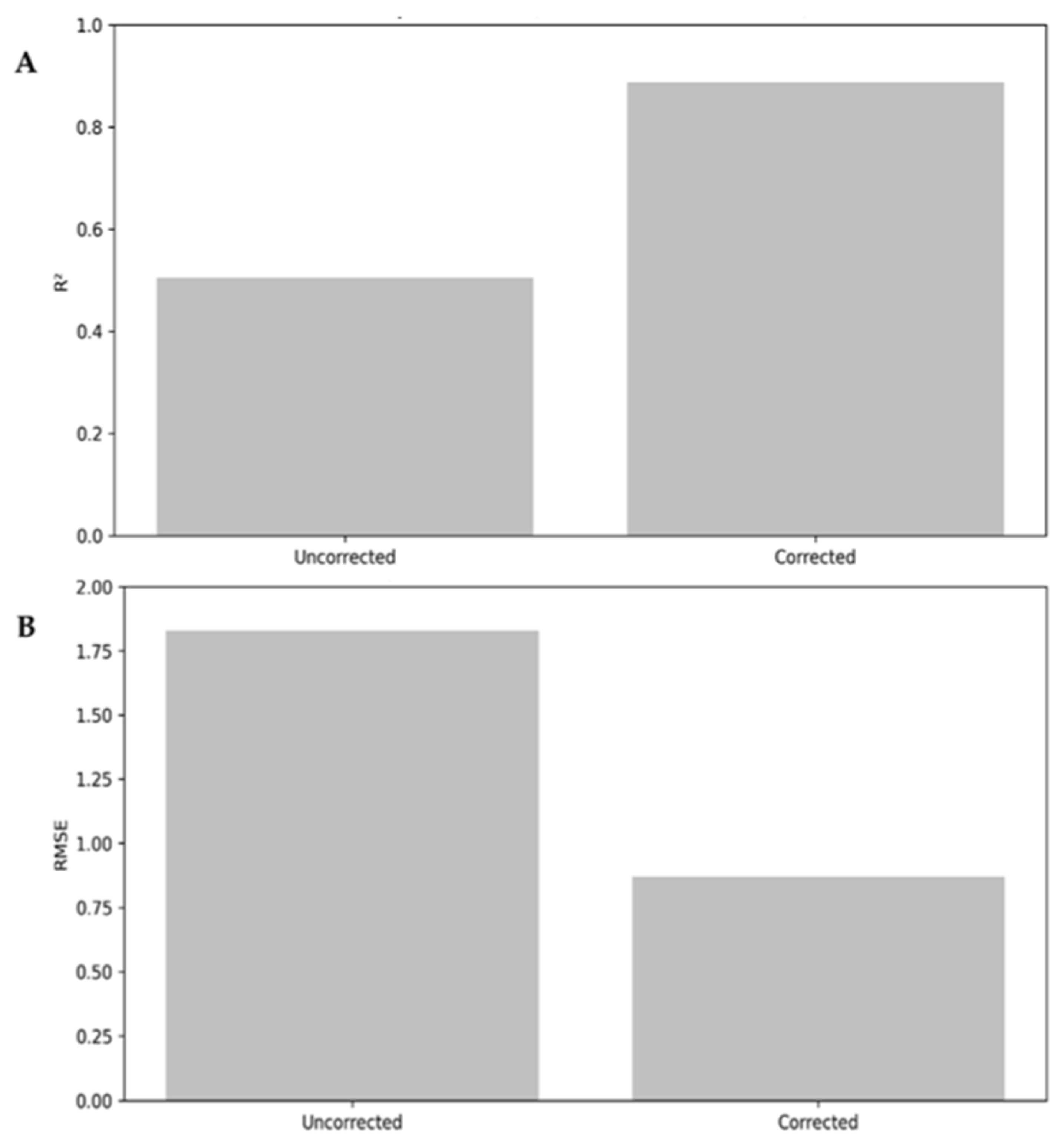
Reevaluation of model metrics: After applying the correction factor, the model evaluation metrics were recalculated, including the coefficient of determination (R²) and the root mean square error (RMSE) (Equations (15) and (16))

$${\mathrm{R}}^2=1-{\displaystyle \frac{{\sum }_{\mathrm{i}=1}^{\mathrm{n}}{(\mathrm{y}}_{\mathrm{i}}-{{\widehat{\mathrm{y}}}_{\mathrm{i}}}^{\mathrm{c}\mathrm{o}\mathrm{r}\mathrm{r}}{)}^2}{{\sum }_{\mathrm{i}=1}^{\mathrm{n}}{(\mathrm{y}}_{\mathrm{i}}-\overline{\mathrm{y}}{)}^2}}$$

(15)

$$\mathrm{R}\mathrm{M}\mathrm{S}\mathrm{E}=\sqrt{{\displaystyle \frac{1}{\mathrm{n}}}{\sum }_{\mathrm{i}=1}^{\mathrm{n}}{(\mathrm{y}}_{\mathrm{i}}-{{\widehat{\mathrm{y}}}_{\mathrm{i}}}^{\mathrm{corr}}{)}^2}$$

(16)

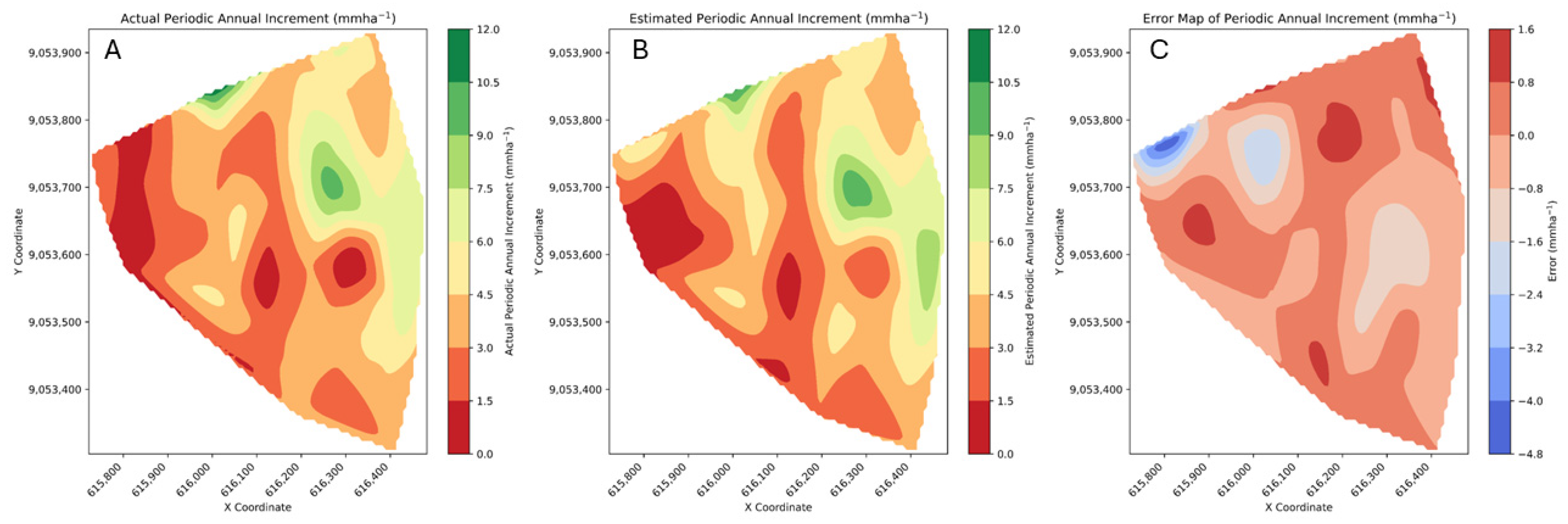
2.9. Generation of Spatial Maps

After constructing the Random Forest models for estimating the Periodic Annual Increment (PAI), spatial distribution maps were generated. The Inverse Distance Weighting (IDW) interpolation technique was used, implemented through the Scipy.interpolate (version 1.10.1, SciPy Developers, Austin, TX, USA) library. This method assigns greater weight to values closer to the predicted location and is well established for the spatial interpolation of environmental variables [78].

The maps were created using both estimated and observed values from the 40 plots. For each plot, the PAI value was interpolated across a grid covering the entire study area using IDW, allowing for the visualization of a spatial continuum of the variables of interest.

IDW was selected due to its simplicity, low computational cost, and suitability for datasets with a limited number of spatial points, as in this case (n = 40 plots). Although geostatistical methods such as Kriging provide estimates of spatial uncertainty, they require assumptions about stationarity and spatial autocorrelation that are difficult to satisfy with small sample sizes.

3. Results and Discussion

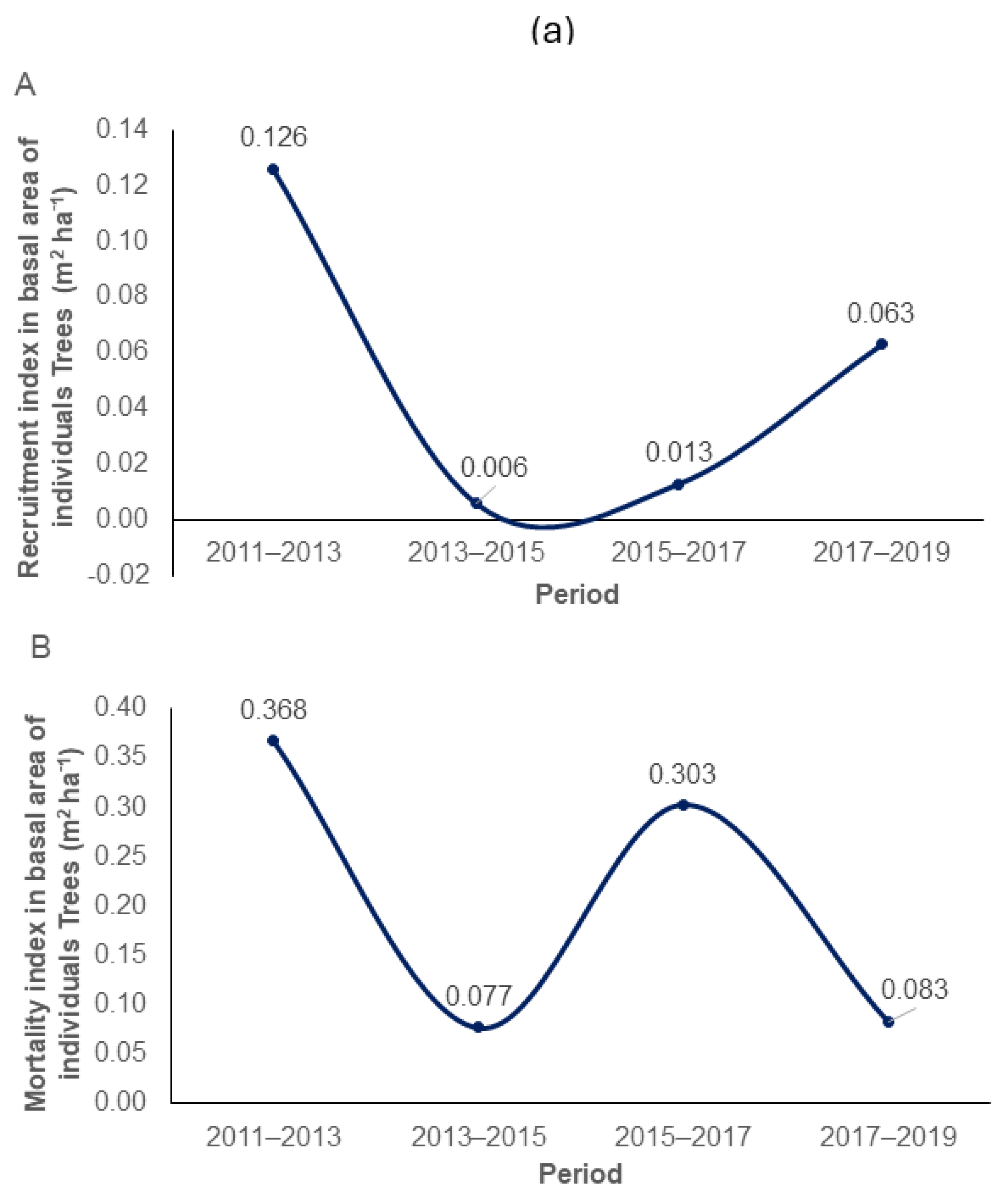
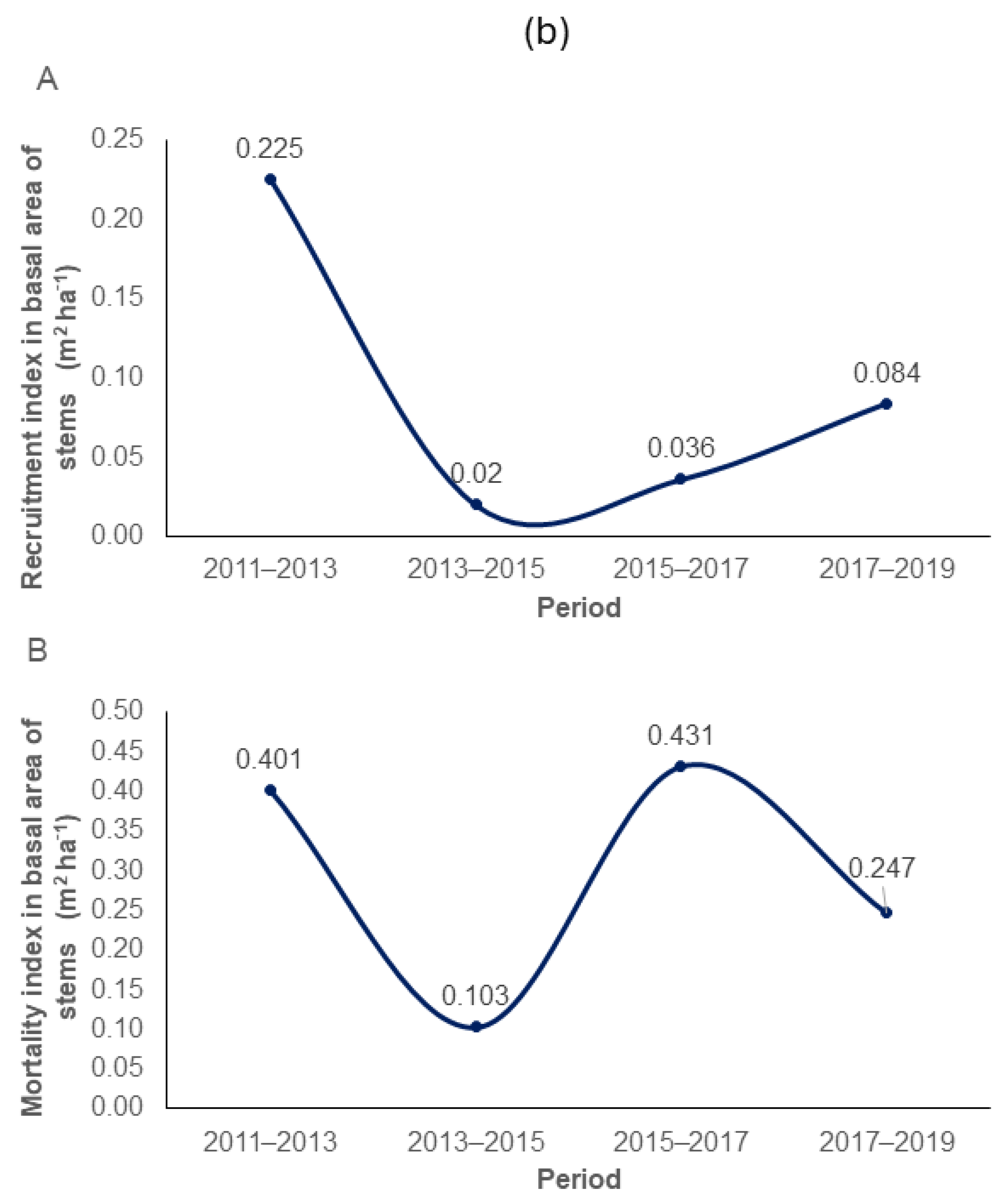
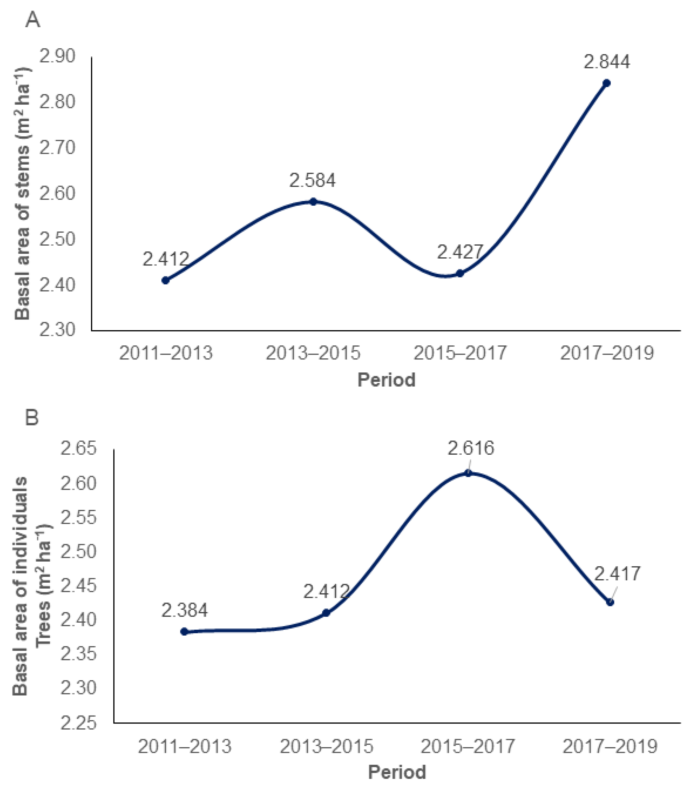
3.1. Growth Dynamics

Figure 3 illustrates the annual variation in precipitation and the minimum, mean, and maximum temperatures in the study area over the years. Based on the graphical analysis, important trends can be observed, helping to contextualize the climatic factors that influence forest growth and the Periodic Annual Increment (PAI) in the Caatinga biome.

Precipitation variability is a defining characteristic of the Caatinga biome, known for its cycles of intense and intermittent droughts. This variability has a direct impact on the Periodic Annual Increment (PAI), as tree growth in the Caatinga is highly dependent on water availability.

Between 2011 and 2019, total mortality in the study area exceeded the recruitment of both stems and individuals (Figure 4a,b and Figure 5). This imbalance resulted in a negative net growth rate, highlighting the struggle for survival faced by various species and individual trees during this period. This timeframe coincided with a severe drought recorded in Northeastern Brazil, which lasted from 2010 to 2016 [5,79]. The recorded water deficit likely had a negative influence on vital plant processes, leading to a reduced growth rate and an increase in vegetation mortality.

The analysis of biennial periods revealed that the maximum basal area increment was recorded in the last analyzed interval, reaching 2.844 m² ha⁻¹ (Figure 5). This growth can be attributed to a reduction in individual mortality and a simultaneous increase in the mortality of smaller stems.

This pattern suggests an adaptive strategy of Caatinga species, in which there is a selective allocation of resources, such as nutrients and water, favoring stems with larger diameters. This natural selection mechanism, known as self-thinning, contributes to the optimization of resource use, promoting the survival and growth of more robust stems.

The higher mortality rate compared to the recruitment of new individuals resulted in a negative net growth for several species between 2011 and 2019. This phenomenon reflects the challenges these species face in developing in this region, as the low recruitment rate significantly impacts the dynamics of the local community (Figure 4). The authors of [54,80] emphasize that population dynamics vary significantly among different species; while some populations respond positively to environmental conditions, others exhibit negative responses. This pattern highlights the complexity and variability inherent in ecological dynamics across different contexts.

Given the semi-arid context, a region frequently affected by intense drought periods, the local vegetation may experience a decline in the number of individuals, leading to an increase in mortality rates. This scenario can result in a negative net growth of populations, as indicated by [81]. The vulnerability of semi-arid flora to such extreme climatic conditions underscores the challenges these ecosystems face in maintaining their integrity and biodiversity.

The predominance of stems over the total number of individuals can be attributed to an adaptive survival mechanism of these species, where bifurcation is a common characteristic among specimens (Figure 6).

A study conducted in the Brazilian Cerrado biome by Ref. [82] demonstrated that wood density significantly influences water translocation within plants. Young plants, characterized by lower wood density, facilitate water transport, contributing to the development of new stems. However, as wood density increases, particularly under high-temperature conditions, water transport efficiency decreases, limiting water availability to certain branches. This process leads to natural pruning, where the less-supplied branches are eliminated, thereby optimizing the distribution of water resources within the plant. Such a process may contribute to woody encroachment, a phenomenon previously recorded in the Cerrado biome [27].

The results of the present study emphasize the complexity and dynamics of the Caatinga biome, addressing key aspects related to recruitment, mortality, basal area, and the Periodic Annual Increment (PAI). The analysis of recruitment highlighted that climatic events, such as precipitation, play a determinant role in vegetation regeneration. This pattern aligns with the findings of Ref. [54], who identified a direct relationship between rainfall occurrence and the recruitment of woody species. In the context of forest management, these data reinforce the importance of considering climatic variability in the development of conservation strategies.

The observed mortality was particularly high during severe drought periods, such as in 2012, confirming previous studies by Ref. [83], which highlighted the vulnerability of Caatinga species to prolonged water deficits. Mortality, combined with recruitment, reflects the high turnover rate of dry tropical forests, showcasing their resilience but also their sensitivity to climate change. Additionally, the mortality and recruitment values indicate the crucial role of interannual precipitation variability; this factor plays a key role in controlling forest dynamics, as discussed by Ref. [84].

The observed forest dynamics patterns were largely influenced by water availability and the edaphic characteristics of the region. Areas with greater hydrological stability exhibited higher recruitment rates, supporting the observations of Ref. [10] regarding the impact of soil resources on the regeneration and growth of woody species. These dynamics are particularly significant in semi-arid regions, where climatic fluctuations play a central role in shaping the structure and composition of forests.

Between 2015 and 2021, Cenostigma bracteosum (Tul.) E. Gagnon & G. P. Lewis exhibited the highest basal area increment, with an average value of 0.210 m² ha⁻¹ year⁻¹ over the analyzed period [3]. Other species with notable growth included Cnidoscolus quercifolius Pohl and Jatropha mollissima (Pohl) Baill, whose PAI in basal area ranged between 0.165 and 0.198 m² ha⁻¹ year⁻¹ from 2018 to 2021, coinciding with slightly higher precipitation levels.

Conversely, some species exhibited negative growth performance throughout this study. Bauhinia cheilantha (Bong.) Steud and Combretum glaucocarpum (Mart.) Eichler recorded negative PAI values in basal area in some periods, with declines of −0.0200 m² ha⁻¹ year⁻¹ and −0.0010 m² ha⁻¹ year⁻¹, respectively.

A study by Ref. [5], conducted between 2011 and 2015, reported lower-diameter PAI values on average compared to the findings of Ref. [3], likely due to the prolonged drought period during that interval. The species Cenostigma bracteosum exhibited the highest basal area increment values, with 0.1217 m² ha⁻¹ year⁻¹ in the 2011–2013 period and 0.0937 m² ha⁻¹ year⁻¹ in 2013–2015. Other species with significant growth included Mimosa ophthalmocentra Mart. ex Benth. and Cnidoscolus quercifolius, which had basal area PAI values of 0.0871 m² ha⁻¹ year⁻¹ and 0.0766 m² ha⁻¹ year⁻¹, respectively.

Some species faced significant regeneration challenges. Combretum glaucocarpum, for instance, recorded a negative basal area PAI of −0.0010 m² ha⁻¹ year⁻¹ between 2013 and 2015. Additionally, between 2011 and 2013, 318 dead individuals and 611 lost stems were recorded, resulting in a mortality rate of 13.51% for individuals and 10.26% for stems. Between 2013 and 2015, the mortality rates decreased to 222 individuals and 501 stems, with mortality rates of 10.71% and 8.46%, respectively.

These results align with the present study, indicating that during periods of greater water scarcity, the species exhibited reduced growth, whereas higher precipitation periods led to increased growth rates.

3.2. Random Forest Model Performance

The statistical analysis of the variables (

Table 2. Descriptive statistics of the analyzed variables for the study area.

Variable	Mean	Median	Min	Max	SD	CV (%)
PAI	4.30	3.94	0.58	16.57	2.59	60.27
Blue	0.06	0.05	0.02	0.09	0.02	32.94
Green	0.09	0.09	0.04	0.14	0.02	25.30
Red	0.12	0.13	0.03	0.20	0.04	36.11
NIR	0.27	0.26	0.19	0.38	0.03	12.89
SWIR1	0.33	0.34	0.18	0.45	0.07	21.48
SWIR2	0.23	0.24	0.08	0.36	0.07	31.81
NDVI	0.38	0.29	0.17	0.82	0.19	50.36
EVI	0.24	0.17	0.10	0.56	0.12	51.61
SAVI	0.25	0.19	0.11	0.54	0.12	46.55
GNDVI	0.49	0.43	0.31	0.76	0.12	24.51
NDWI	−0.10	−0.16	−0.29	0.31	0.15	−160.12
NDBI	0.10	0.16	−0.31	0.29	0.15	160.12
MSI	1.27	1.38	0.53	1.83	0.35	27.33
NBR	0.10	0.03	−0.19	0.62	0.21	214.83
NDSI	−0.57	−0.56	−0.64	−0.51	0.02	−4.36
LAI	0.95	0.93	0.67	1.35	0.13	13.31

) considered in this study included mean, median, minimum and maximum values, standard deviation (SD), and coefficient of variation (CV%). These metrics were calculated for the Periodic Annual Increment (PAI), vegetation indices, and spectral bands obtained from Landsat 5 and Landsat 8 satellite images.

The Periodic Annual Increment (PAI) had an average of 4.30 mm.ha⁻¹ and a median of 3.94 mm.ha⁻¹, with significant variation between the minimum (0.58 mm.ha⁻¹) and maximum (16.57 mm.ha⁻¹) values, reflected in the high coefficient of variation (CV) of 60.27%.

Among the spectral bands, the NIR (related to cell wall structure) and SWIR1 (associated with leaf water content) exhibited lower coefficients of variation, 12.89% and 21.48%, respectively, suggesting greater stability in reflectance values. On the other hand, indices such as NDBI and NBR displayed extremely high coefficients of variation, 160.12% and 214.83%, respectively, indicating greater variability, possibly due to the structural heterogeneity of the study area.

The EVI and SAVI indices, known for their sensitivity to vegetation, showed relatively high coefficients of variation, 51.61% and 46.55%, respectively, highlighting the spatial and temporal variability in vegetation in the analyzed area. Additionally, SAVI has been recognized as suitable for areas with low vegetation cover, as described in [85]. This index proved useful for biomass modeling in semi-arid ecosystems. Furthermore, the NDWI water index exhibited a contrasting behavior, with a negative mean value (−0.10) and a high coefficient of variation (−160.12%), possibly linked to the restricted water conditions of the semi-arid region, consistent with the findings of Ref. [86]. These authors explored the seasonal dynamics of water resources in dry tropical forests, emphasizing the vegetation response to limited water availability and the challenges in detecting critical areas within semi-arid ecosystems.

The variability observed in spectral indices, such as the NDVI and EVI, reinforces the importance of these indices in analyzing the structural heterogeneity and vegetation dynamics in dry ecosystems. The high coefficients of variation (CV = 50.36% for NDVI) found in this study reflect the complexity and structural heterogeneity of the Caatinga, characteristics that have also been described in remote sensing analyses of seasonal tropical forests.

The NDVI is widely used to represent seasonal differences in vegetation, whereas the EVI is effective in correcting soil influences, especially in heterogeneous areas [85]. This index was useful for biomass modeling in semi-arid ecosystems, which is consistent with our results, where the Caatinga, characterized by sparse vegetation and seasonal variability, exhibited high variability in these indices.

The lower coefficients of variation observed for the NIR (12.89%) and SWIR1 (21.48%) spectral bands further emphasize the importance of these variables in capturing information related to biomass and vegetation health. This behavior reflects the direct interaction of these bands with leaf structure and vegetation density, as highlighted by Ref. [43], who demonstrated the critical role of NIR, along with the red-edge band, in distinguishing vegetation types and understanding their interactions with soil attributes in the Brazilian semi-arid region.

Overall, the variability expressed by the coefficients of variation reflects the intrinsic heterogeneity of vegetation, environmental conditions, and spectral indices in the study area, reinforcing the complexity of monitoring dry tropical forests. These results highlight the importance of robust methods, such as the use of machine learning algorithms, for data modeling and analysis.

The selection of variables based on Spearman’s correlation allowed for a significant reduction in the number of spectral variables and vegetation indices used in the predictive model for the Periodic Annual Increment (PAI). Initially, 16 variables were evaluated, of which only four showed statistically significant correlations (p < 0.05) with PAI (

Table 3. Significant correlations between variables and the Periodic Annual Increment (PAI) for model construction.

Variable	Correlation	p-Value
NIR	0.254451	0.000004
LAI	0.244708	0.000010
NDSI	0.201745	0.000281
NDVI	0.118065	0.034761

).

Among the selected variables, NIR (Near Infrared) exhibited the highest correlation (r = 0.254, p = 0.000004), standing out as the most strongly related variable to the Periodic Annual Increment (PAI). This result aligns with the role of NIR in capturing information on biomass and vegetation health, reflecting its interaction with leaf structure and vegetation density [43]. These findings are consistent with those of Ref. [87], which demonstrated that Landsat 8 spectral bands, such as NIR, possess high predictive capacity in forest ecosystems due to their sensitivity to structural characteristics and vegetation health.

Additionally, Ref. [88] emphasized the importance of NIR in capturing leaf structure-related information, such as chlorophyll content and physical leaf characteristics, which are essential for distinguishing between different vegetation types. These findings support the strong correlation observed between NIR and PAI (r = 0.254) in the present study, reinforcing its role as a key predictor variable in modeling vegetation productivity.

The Leaf Area Index (LAI) also showed a significant correlation (r = 0.245, p = 0.000010), further reinforcing its importance in PAI modeling, as LAI is directly related to primary vegetation productivity and growth dynamics.

The Normalized Difference Snow Index (NDSI) presented a moderate correlation (r = 0.202, p = 0.000281), suggesting that the model is sensitive to soil and vegetation properties in arid environments, where reflectance conditions may be influenced by leafless vegetation. Etymologically, the word “Caatinga” (Brazilian Dry Tropical Forest) originates from the Tupi-Guarani language and means “white forest”, composed of caa (forest) and tinga (white).

The NDVI (Normalized Difference Vegetation Index), widely used as an indicator of vegetation cover, exhibited a relatively low but significant correlation (r = 0.118, p = 0.034761), indicating its contribution to the model despite its weaker association with PAI. This behavior aligns with the findings of [74] who demonstrated that NDVI is effective in differentiating vegetation classes. It is also consistent with the results of [89], who highlighted NDVI’s sensitivity to climatic variations in semi-arid regions of Northeastern Brazil over a 20-year period. Their study identified that NDVI captures both seasonal and interannual vegetation patterns, reflecting changes in vegetation cover in response to climatic and environmental fluctuations.

The reduction in the number of variables based on correlation criteria not only simplifies the model but also reduces potential multicollinearity issues, ensuring greater efficiency and interpretability in the predictive modeling process. These results highlight the importance of selecting key variables that capture the most relevant variations in forest growth dynamics, particularly in complex ecosystems such as dry tropical forests.

The vegetation indices and the NIR band used in this study demonstrated a positive correlation with PAI, confirming their utility as proxies for estimating vegetation productivity. Ref. [84] previously highlighted the robustness of using remote sensing data to capture variations in vegetation cover and vigor. The Spearman correlation analysis revealed that remote sensing-derived variables had significant relationships with PAI, supporting the findings of Ref. [10], who emphasized the role of these indicators in modeling forest processes.

The reduction in the number of variables based on correlation criteria not only simplifies the model but also reduces potential multicollinearity issues, ensuring greater efficiency and interpretability in the predictive modeling process. As emphasized by Ref. [90], Spearman’s correlation coefficient is a robust tool for identifying monotonic associations between variables, especially when data do not meet normality or linearity assumptions. By replacing original values with ranks, Spearman’s method allows for reliable analysis, even in cases of asymmetrical distributions, which are frequently observed in environmental data.

The initial evaluation of the Random Forest model for estimating PAI showed promising results, but also highlighted challenges related to the intrinsic variability in field data. Before applying adjustments, the model presented a coefficient of determination (R²) of 0.5055, indicating that approximately 50.55% of the variation in actual PAI values was explained by the model, while the Root Mean Square Error (RMSE) was 1.83 mm.ha⁻¹. These results are consistent with the performance reported by Ref. [91] in arid regions, where Random Forest was identified as the most accurate algorithm for predicting environmental and soil properties in challenging scenarios with high dimensionality and correlated variables.

The study by Ref. [87] further supports the potential of Random Forest as a powerful tool for environmental modeling, even when compared to more recent algorithms such as XGBoost. The ability of Random Forest to randomly sample variables and observations enhances its resistance to multicollinearity, enabling more effective modeling in complex ecosystems.

An analysis of the estimated values revealed that the model tended to underestimate higher PAI values and overestimate lower ones, as evidenced by an average percentage difference of 0.29% and a total absolute difference of 4.00 mm.ha⁻¹. This bias may be attributed to the structural complexity of the dry tropical forest and the model’s limitations in fully capturing the variability in spectral and vegetation index data.

The initial challenges of the model included the underestimation of high PAI values and overestimation of low PAI values, a behavior also observed by Ref. [87] in forest biomass estimations using Random Forest. This limitation is attributed to the algorithm’s difficulty in handling extreme data points without additional adjustments. Nonetheless, the high Spearman’s correlation (0.846) demonstrated that the model effectively captured general data trends, even though it lacked precision in extreme values.

The application of Random Forest for drought monitoring in grasslands has highlighted that adjustments based on error distribution can minimize discrepancies and improve overall model performance, a strategy that has also been implemented in the present study [92].

Given this limitation, a correction factor was introduced, based on the distribution of estimation errors. The adjustment involved dividing the data into six classes, using PAI value intervals, and computing average correction factors for each class. These factors were then applied to adjust the model’s estimated values, resulting in a substantial improvement in prediction accuracy (

Table 4. Correction factor for model bias in estimating the Periodic Annual Increment (PAI) (mm.ha⁻¹).

Class	Intervals (mm.ha−1)	Correction Factor (FC)
1	0.5835–1.8916	−0.8685
2	1.8916–2.9572	−0.6340
3	2.9572–3.9390	−0.4750
4	3.9390–4.8921	−0.1901
5	4.8921–6.4431	0.2911
6	6.4431–16.5665	1.5334

).

After applying the correction factor, the model’s results were significantly improved. The R² increased to 0.8867, indicating that 88.67% of the variation in the actual PAI values is now explained by the corrected model. This substantial increase in R² reflects a better fit between the estimated and real values. Simultaneously, the RMSE was reduced to 0.87 mm.ha⁻¹, demonstrating a marked reduction in the average prediction error (Figure 7).

This outcome aligns with the findings of Refs. [93,94], who underscored the importance of post-modeling adjustments in reducing discrepancies in heterogeneous systems. Moreover, the use of correction factors reinforces the applicability of Random Forest in complex scenarios, such as dry tropical forests. Ref. [85] highlighted the algorithm’s capacity to capture complex patterns and handle nonlinear data, demonstrating its relevance for robust estimates in heterogeneous ecosystems.

Furthermore, Spearman’s correlation increased to 0.946 after applying the correction factor, indicating a more robust relationship between the actual and estimated values. This improvement not only reflects enhanced metrics such as R² and RMSE but also demonstrates greater consistency in the ranking trends of the corrected data, which is crucial for monitoring and management studies. The high post-correction correlation shows that the adjusted model is capable of capturing the patterns of forest growth with higher fidelity, even in an environment characterized by high variability.

Figure 8 presents detailed comparisons between the actual and estimated values of the Periodic Annual Increment (PAI) before and after the Random Forest model correction. Density analyses reveal improved alignment between the estimated and actual values after applying the correction factor. The distribution peaks become closer, indicating a significant reduction in the discrepancy between the estimated maximum and minimum values.

Scatter plots further illustrate the relationship between the actual and estimated values before and after correction. It is evident that, following the application of the correction factor, the values align more consistently, signifying a substantial improvement in the model’s predictive accuracy.

These results underscore the effectiveness of the correction factor in adjusting discrepancies—especially in extreme values—thereby enhancing the model’s ability to capture the variations in forest growth within the study area.

Post-modeling adjustments are essential for addressing discrepancies in predictions for complex systems such as dry tropical forests. The application of correction factors allows estimates to be aligned with observed data, particularly in cases where data variability challenges traditional modeling approaches [95]. The corrected model demonstrated significantly improved performance, underscoring its potential as a valuable tool for the management and monitoring of dry tropical forests. Furthermore, the strong correlation between precipitation and PAI (r = 0.946) suggests that environmental factors, such as water availability, play a crucial role in forest growth and should be incorporated into future studies to refine predictive estimates.

Table 5. Precipitation and PAI values for the studied periods.

Period	Mean Precipitation (mm)	Mean PAI (mm)
2011–2013	286.2	4.04
2013–2015	245.9	3.73
2015–2017	372.5	4.23
2017–2019	461.7	6.14

shows that there is a positive relationship between precipitation and PAI, with periods of higher precipitation being associated with higher mean PAI values. This indicates that precipitation may be an important factor in tree growth in the Caatinga, a biome sensitive to moisture variations. Similar results were found by Ref. [96], who demonstrated the significant influence of precipitation on the seasonality of vegetation in the Caatinga biome, reinforcing the biome’s sensitivity to water availability Ref. [97].

The values between the mean precipitation and the mean Periodic Annual Increment (PAI) exhibited a correlation of approximately 0.92. This indicates a strong positive correlation, suggesting that, in this dataset, periods with higher precipitation tend to be associated with higher tree growth rates. According to recent studies, precipitation plays a crucial role in the population dynamics of Caatinga vegetation. Ref. [98] found that the growth of woody species in the Brazilian semi-arid region is directly influenced by water availability, especially in years with above-average precipitation patterns.

Furthermore, research conducted by Ref. [99] highlighted that the Leaf Area Index and biomass of the Caatinga are strongly dependent on precipitation patterns, demonstrating that water availability is a limiting factor for vegetation development. These findings align with the observations in Table 5, which reinforce the importance of precipitation as one of the main determining factors for the Periodic Annual Increment in trees in the Caatinga.

Periods with below-average precipitation, such as those observed in 2012 and 2014, tend to result in lower mean PAI values, as previously shown. Conversely, years with greater water availability, such as 2019, coincide with higher forest growth rates, reinforcing the strong positive correlation between precipitation and PAI (ρ = 0.92).

The combination of highly variable precipitation and elevated temperatures creates a challenging environment for forest growth in the Caatinga biome. These factors underscore the need to consider not only water availability but also the role of extreme temperatures in adjusting and refining predictive models of PAI. Additionally, these climatic data provide a basis for exploring adaptive management strategies that can mitigate the effects of climate change on the growth of tree species in this ecosystem.

The Periodic Annual Increment (PAI), a widely used metric for evaluating forest growth, revealed significant variations over the analyzed years. The PAI values were lower during dry periods and higher in years with above-average precipitation, as observed in 2019. This pattern is consistent with the physiological response mechanisms of species to water deficits, as discussed by Refs. [7,83]. Mapping the PAI revealed marked spatial variations, reflecting the interactions between climatic and edaphic factors, as also observed by Ref. [100] in a similar study.

The positive relationship between precipitation and the PAI, with a correlation of 0.92, reinforces the importance of water availability for tree growth in the Caatinga, as evidenced by studies from Refs. [101,102]. This result highlights the need for continuous monitoring of climatic conditions and their incorporation into forest management models to mitigate the impacts of climate change.

The analysis of these climatic factors demonstrates the relevance of using robust models—such as the corrected Random Forest—to estimate the PAI, incorporating environmental variables and their interactions. The variability in precipitation and the persistence of high temperatures underscore the importance of continuously monitoring climatic conditions in the sustainable management of the Caatinga.

The spatial distribution maps of the actual and estimated PAI, along with the uncertainty map, provided valuable insights into the forest dynamics of the region (Figure 9). It was observed that areas with higher species diversity and closer proximity to recharge sources exhibited the highest increments, while plots located in more arid areas showed the largest estimation errors. This pattern highlights the importance of integrating climatic and edaphic data to refine predictions, as suggested by Ref. [103]. In the error map, the greatest discrepancies were associated with specific plots, which may be related to species diversity and local growth dynamics.

4. Conclusions

The estimates generated by the Random Forest model showed high agreement with the field data, demonstrating its efficacy in predicting the Periodic Annual Increment (PAI) in dry tropical forests. The application of a correction factor to the model was decisive in improving the precision of the estimates, resulting in a significant increase in the coefficient of determination (R²) and a reduction in the root mean square error (RMSE). This adjustment underscores the importance of integrating post-processing methods in forest modeling studies, particularly in ecosystems with high spatial and temporal variability.

This work demonstrates that the integration of remote sensing, machine learning, and field data is an effective approach for understanding the forest dynamics of the Caatinga. In addition to contributing to scientific advancement in the field, the results presented provide important support for the planning and sustainable management of this biome in the context of climate change.

Despite the promising results, this study presents limitations that should be acknowledged. The relatively small number of sampling plots (n = 40) may limit the generalization of the model to broader spatial scales. In addition, the model was calibrated using spectral and climatic conditions specific to the study area, which may differ across other regions or under varying seasonal contexts. Future research should consider integrating additional environmental variables (e.g., soil texture, land use history) and expanding the spatial and temporal extent of data collection to improve model accuracy and applicability in other ecosystems.

References

1. Perrando, E.R.; Breunig, F.M.; Galvão, L.S.; Bostelmann, S.L.; Martarello, V.; Straube, J.; Conte, B.; Sestari, G.; Burgin, M.R.B.; De Marco, R. Evaluation of the Effects of Pine Management on the Water Yield and Quality in Southern Brazil. J. Sustain. For. 2021, 40, 217–233. [Google Scholar] [CrossRef]
2. Kumar Mishra, R.; Agarwal, R. Sustainable Forest Land Management to Restore Degraded Lands; IntechOpen: Rijeka, Croatia, 2024. [Google Scholar] [CrossRef]
3. Da Silva, A.F. Estrutura e Dinâmica Relacionadas A Fatores Ambientais em Floresta Seca Submetida ao Manejo Florestal. Ph.D. Thesis, Universidade Federal Rural de Pernambuco, Recife, Brazil, 2023. [Google Scholar]
4. Salazar, A.A.; Arellano, E.C.; Muñoz-sáez, A.; Miranda, M.D.; da Silva, F.O.; Zielonka, N.B.; Crowther, L.P.; Silva-ferreira, V.; Oliveira-reboucas, P.; Dicks, L.V. Restoration and Conservation of Priority Areas of Caatinga’s Semi-Arid Forest Remnants Can Support Connectivity within an Agricultural Landscape. Land 2021, 10, 550. [Google Scholar] [CrossRef]
5. De Melo, C.L.S.M.S.; Ferreira, R.L.C.; da Silva, J.A.A.; Machuca, M.Á.H.; Cespedes, G.H.G. Dynamics of Dry Tropical Forest after Three Decades of Vegetation Suppression. Floresta Ambient. 2019, 26, e20171163. [Google Scholar]
6. dos Santos, N.Á.T. Dinâmica da Floresta Seca SOB Diferentes Históricos de USO: Distribuição Diamétrica de Indivíduos e Fustes. Master’s Thesis, Universidade Federal Rural de Pernambuco, Recife, Brazil, 2021. [Google Scholar]
7. Dalla Lana, M.; Ferreira, R.L.C.; da Silva, J.A.A.; Duda, G.P.; Cespedes, G.H.G. Carbon Content in Shrub-Tree Species of the Caatinga. Floresta Ambient. 2019, 26, e20170617. [Google Scholar] [CrossRef]
8. De Abreu, J.C.; da Silva, J.A.A.; Ferreira, R.L.C.; da Rocha, S.J.S.S.; Tavares, I.d.S.; Farias, A.A.; Villanova, P.H.; Viana, A.B.T.; Schettini, B.L.S.; Telles, L.A.d.A.; et al. Mixed Models for Nutrients Prediction in Species of the Brazilian Caatinga Biome. Árvore 2023, 47, e4712. [Google Scholar] [CrossRef]
9. Salami, G.; Ferreira, R.L.C.; da Silva, J.A.A.; Freire, F.J.; Silva, E.A.; Diodato, M.A.; Pessi, D.D. Distribuição Espaço-Temporal Da Biomassa e Carbono Florestal Acima Do Solo Em Floresta Tropical Seca Sob Pressão Antrópica, Brasil. Terr@ Plur. 2024, 18, 1–27. [Google Scholar] [CrossRef]
10. Moreira, G.L. Modelagem de Variáveis Biofísicas Em Floresta Tropical Seca Por Meio de Geotecnologias. Master’s Thesis, Universidade Federal Rural de Pernambuco, Recife, Brasil, 2021. [Google Scholar]
11. de Oliveira, C.P.; Ferreira, R.L.C.; da Silva, J.A.A.; de Lima, R.B.; Silva, E.A.; da Silva, A.F.; de Lucena, J.D.S.; Dos Santos, N.A.T.; Lopes, I.J.C.; Pessoa, M.M.d.L.; et al. Modeling and Spatialization of Biomass and Carbon Stock Using LiDAR Metrics in Tropical Dry Forest, Brazil. Forests 2021, 12, 473. [Google Scholar] [CrossRef]
12. Beck, H.E.; McVicar, T.R.; Vergopolan, N.; Berg, A.; Lutsko, N.J.; Dufour, A.; Zeng, Z.; Jiang, X.; van Dijk, A.I.J.M.; Miralles, D.G. High-Resolution (1 Km) Köppen-Geiger Maps for 1901–2099 Based on Constrained CMIP6 Projections. Sci. Data 2023, 10, 724. [Google Scholar] [CrossRef]
13. Ottoni, F.P.; Filgueira, C.T.S.; Lima, B.N.; Vieira, L.O.; Rangel-Pereira, F.; Oliveira, R.F. Extreme Drought Threatens the Amazon. Science 2023, 382, 1253–1255. [Google Scholar] [CrossRef]
14. AR6 Synthesis Report: Climate Change 2023. Available online: https://www.ipcc.ch/report/ar6/syr/ (accessed on 20 March 2025).
15. Santos, J.C.; Leal, I.R.; Almeida-Cortez, J.S.; Fernandes, G.W.; Tabarelli, M. Caatinga: The Scientific Negligence Experienced by a Dry Tropical Forest. Trop. Conserv. Sci. 2011, 4, 276–286. [Google Scholar] [CrossRef]
16. Leal, I.R.; Da Silva, J.M.C.; Tabarelli, M.; Lacher, T.E. Changing the Course of Biodiversity Conservation in the Caatinga of Northeastern Brazil Cambiando El Curso de La Conservación de Biodiversidad En La Caatinga Del Noreste de Brasil. Conserv. Biol. 2005, 19, 701–706. [Google Scholar] [CrossRef]
17. Pitman, N.C.A.; Silman, M.R.; Terborgh, J.W. Oligarchies in Amazonian Tree Communities: A Ten-Year Review. Ecography 2013, 36, 114–123. [Google Scholar] [CrossRef]
18. Ter Steege, H.; Pitman, N.C.A.; Sabatier, D.; Baraloto, C.; Salomão, R.P.; Guevara, J.E.; Phillips, O.L.; Castilho, C.V.; Magnusson, W.E.; Molino, J.F.; et al. Hyperdominance in the Amazonian Tree Flora. Science 2013, 342, 1243092. [Google Scholar] [CrossRef] [PubMed]
19. Bonal, D.; Burban, B.; Stahl, C.; Wagner, F.; Hérault, B. The Response of Tropical Rainforests to Drought—Lessons from Recent Research and Future Prospects. Ann. For. Sci. 2016, 73, 27–44. [Google Scholar] [CrossRef]
20. Elias, F.; Marimon, B.S.; Marimon-Junior, B.H.; Budke, J.C.; Esquivel-Muelbert, A.; Morandi, P.S.; Reis, S.M.; Phillips, O.L. Idiosyncratic Soil-Tree Species Associations and Their Relationships with Drought in a Monodominant Amazon Forest. Acta Oecol. 2018, 91, 127–136. [Google Scholar] [CrossRef]
21. Lloyd, J.; Domingues, T.F.; Schrodt, F.; Ishida, F.Y.; Feldpausch, T.R.; Saiz, G.; Quesada, C.A.; Schwarz, M.; Torello-Raventos, M.; Gilpin, M.; et al. Edaphic, Structural and Physiological Contrasts across Amazon Basin Forest-Savanna Ecotones Suggest a Role for Potassium as a Key Modulator of Tropical Woody Vegetation Structure and Function. Biogeosciences 2015, 12, 6529–6571. [Google Scholar] [CrossRef]
22. Powers, J.S.; Feng, X.; Sánches-Azofeifa, A.; Medvigy, D. Focus on tropical dry forest ecosystems and ecosystem services in the face of global change. Environ. Res. Lett. 2018, 13, e090201. [Google Scholar] [CrossRef]
23. Dickinson, M.B.; Hermann, S.M.; Whigham, D.F. Low Rates of Background Canopy-Gap Disturbance in a Seasonally Dry Forest in the Yucatan Peninsula with a History of Fires and Hurricanes. J. Trop. Ecol. 2001, 17, 895–902. [Google Scholar] [CrossRef]
24. Doe Santos, J.R.; Narvaes, I.S.; Graca, P.M.L.A.; Goncalves, F.G.; dos Santos, J.R.; Narvaes, I.S.; Graca, P.M.L.A.; Goncalves, F.G. Polarimetric Responses and Scattering Mechanisms of Tropical Forests in the Brazilian Amazon. In Advances in Geoscience and Remote Sensing; Intechopen: Rijeka, Croatia, 2009. [Google Scholar] [CrossRef]
25. da Conceição Bispo, P.; Picoli, M.C.A.; Marimon, B.S.; Marimon Junior, B.H.; Peres, C.A.; Menor, I.O.; Silva, D.E.; de Figueiredo Machado, F.; Alencar, A.A.C.; de Almeida, C.A.; et al. Overlooking Vegetation Loss Outside Forests Imperils the Brazilian Cerrado and Other Non-Forest Biomes. Nat. Ecol. Evol. 2023, 8, 12–13. [Google Scholar] [CrossRef]
26. Chave, J.; Réjou-Méchain, M.; Búrquez, A.; Chidumayo, E.; Colgan, M.S.; Delitti, W.B.C.; Duque, A.; Eid, T.; Fearnside, P.M.; Goodman, R.C.; et al. Improved Allometric Models to Estimate the Aboveground Biomass of Tropical Trees. Glob. Change Biol. 2014, 20, 3177–3190. [Google Scholar] [CrossRef]
27. Rosan, T.M.; Aragão, L.E.O.C.; Oliveras, I.; Phillips, O.L.; Malhi, Y.; Gloor, E.; Wagner, F.H. Extensive 21st-Century Woody Encroachment in South America’s Savanna. Geophys. Res. Lett. 2019, 46, 6594–6603. [Google Scholar] [CrossRef]
28. Raymundo, D.; Oliveira-Neto, N.E.; Martini, V.; Araújo, T.N.; Calaça, D.; de Oliveira, D.C. Assessing Woody Plant Encroachment by Comparing Adult and Juvenile Tree Components in a Brazilian Savanna. Flora 2022, 291, 152060. [Google Scholar] [CrossRef]
29. Bilar, A.B.C.; Pimentel, R.M.d.M.; Cerqueira, M.A. Monitoramento Da Cobertura Vegetal Através de Índices Biofísicos e Gestão de Áreas Protegidas. Geosul 2018, 33, 236–259. [Google Scholar] [CrossRef]
30. García-Haro, F.J.; Campos-Taberner, M.; Muñoz-Marí, J.; Laparra, V.; Camacho, F.; Sánchez-Zapero, J.; Camps-Valls, G. Derivation of Global Vegetation Biophysical Parameters from EUMETSAT Polar System. ISPRS J. Photogramm. Remote Sens. 2018, 139, 57–74. [Google Scholar] [CrossRef]
31. Piles, M.; Camps-Valls, G.; Chaparro, D.; Entekhabi, D.; Konings, A.G.; Jagdhuber, T. Remote Sensing of Vegetation Dynamics in Agro-Ecosystems Using Smap Vegetation Optical Depth and Optical Vegetation Indices. In Proceedings of the International Geoscience and Remote Sensing Symposium (IGARSS), Fort Worth, TX, USA, 23–28 July 2017; pp. 4346–4349. [Google Scholar] [CrossRef]
32. Verrelst, J.; Malenovský, Z.; Van der Tol, C.; Camps-Valls, G.; Gastellu-Etchegorry, J.P.; Lewis, P.; North, P.; Moreno, J. Quantifying Vegetation Biophysical Variables from Imaging Spectroscopy Data: A Review on Retrieval Methods. Surv. Geophys. 2019, 40, 589–629. [Google Scholar] [CrossRef]
33. Gutiérrez-Castorena, E.V.; Silva-Núñez, J.A.; Gaytán-Martínez, F.D.; Encinia-Uribe, V.V.; Ramírez-Gómez, G.A.; Olivares-Sáenz, E. Evaluation of Statistical Models of NDVI and Agronomic Variables in a Protected Agriculture System. Horticulturae 2025, 11, 131. [Google Scholar] [CrossRef]
34. Albuquerque, R.W.; Ferreira, M.E.; Olsen, S.I.; Tymus, J.R.C.; Balieiro, C.P.; Mansur, H.; Moura, C.J.R.; Costa, J.V.S.; Branco, M.R.C.; Grohmann, C.H. Forest Restoration Monitoring Protocol with a Low-Cost Remotely Piloted Aircraft: Lessons Learned from a Case Study in the Brazilian Atlantic Forest. Remote Sens. 2021, 13, 2401. [Google Scholar] [CrossRef]
35. John, E.; Bunting, P.; Hardy, A.; Silayo, D.S.; Masunga, E. A Forest Monitoring System for Tanzania. Remote Sens. 2021, 13, 3081. [Google Scholar] [CrossRef]
36. Wulder, M.A.; White, J.C.; Masek, J.G.; Dwyer, J.; Roy, D.P. Continuity of Landsat Observations: Short Term Considerations. Remote Sens. Environ. 2011, 115, 747–751. [Google Scholar] [CrossRef]
37. Asner, G.P.; Powell, G.V.N.; Mascaro, J.; Knapp, D.E.; Clark, J.K.; Jacobson, J.; Kennedy-Bowdoin, T.; Balaji, A.; Paez-Acosta, G.; Victoria, E.; et al. High-Resolution Forest Carbon Stocks and Emissions in the Amazon. Proc. Natl. Acad. Sci. USA 2010, 107, 16738–16742. [Google Scholar] [CrossRef]
38. Saatchi, S.S.; Harris, N.L.; Brown, S.; Lefsky, M.; Mitchard, E.T.A.; Salas, W.; Zutta, B.R.; Buermann, W.; Lewis, S.L.; Hagen, S.; et al. Benchmark Map of Forest Carbon Stocks in Tropical Regions across Three Continents. Proc. Natl. Acad. Sci. USA 2011, 108, 9899–9904. [Google Scholar] [CrossRef] [PubMed]
39. Mitchard, E.T.A.; Flintrop, C.M. Woody Encroachment and Forest Degradation in Sub-Saharan Africa’s Woodlands and Savannas 1982–2006. Philos. Trans. R. Soc. B Biol. Sci. 2013, 368, 20120406. [Google Scholar] [CrossRef] [PubMed]
40. Berra, E.F.; Fontana, D.C.; Yin, F.; Breunig, F.M. Harmonized Landsat and Sentinel-2 Data with Google Earth Engine. Remote Sens. 2024, 16, 2695. [Google Scholar] [CrossRef]
41. Claverie, M.; Ju, J.; Masek, J.G.; Dungan, J.L.; Vermote, E.F.; Roger, J.C.; Skakun, S.V.; Justice, C. The Harmonized Landsat and Sentinel-2 Surface Reflectance Data Set. Remote Sens. Environ. 2018, 219, 145–161. [Google Scholar] [CrossRef]
42. Breiman, L. Random Forests. Mach. Learn. 2001, 45, 5–32. [Google Scholar] [CrossRef]
43. da Silveira, H.L.F.; Galvão, L.S.; Sanches, I.D.A.; de Sá, I.B.; Taura, T.A. Use of MSI/Sentinel-2 and Airborne LiDAR Data for Mapping Vegetation and Studying the Relationships with Soil Attributes in the Brazilian Semi-Arid Region. Int. J. Appl. Earth Obs. Geoinf. 2018, 73, 179–190. [Google Scholar] [CrossRef]
44. Hastie, T.; Tibshirani, R.; Friedman, J. The Elements of Statistical Learning; Springer: Berlin/Heidelberg, Germany, 2009. [Google Scholar] [CrossRef]
45. Goodfellow, I.; Bengio, Y.; Courville, A. Deep Learning; The MIT Press: London, UK, 2016. [Google Scholar]
46. Zhang, J.; Yin, K. Application of Gradient Boosting Model to Forecast Corporate Green Innovation Performance. Front. Environ. Sci. 2023, 11, 1252271. [Google Scholar] [CrossRef]
47. Rodriguez-Galiano, V.F.; Ghimire, B.; Rogan, J.; Chica-Olmo, M.; Rigol-Sanchez, J.P. An Assessment of the Effectiveness of a Random Forest Classifier for Land-Cover Classification. ISPRS J. Photogramm. Remote Sens. 2012, 67, 93–104. [Google Scholar] [CrossRef]
48. Powell, S.L.; Cohen, W.B.; Healey, S.P.; Kennedy, R.E.; Moisen, G.G.; Pierce, K.B.; Ohmann, J.L. Quantification of Live Aboveground Forest Biomass Dynamics with Landsat Time-Series and Field Inventory Data: A Comparison of Empirical Modeling Approaches. Remote Sens. Environ. 2010, 114, 1053–1068. [Google Scholar] [CrossRef]
49. Cutler, D.R.; Edwards, T.C.; Beard, K.H.; Cutler, A.; Hess, K.T.; Gibson, J.; Lawler, J.J. Random Forests for Classification in Ecology. Ecology 2007, 88, 2783–2792. [Google Scholar] [CrossRef]
50. Liaw, A.; Wiener, M. Classification and Regression by RandomForest. R News 2002, 2, 18–22. [Google Scholar]
51. Machado, G.; Mendoza, M.R.; Corbellini, L.G. What Variables Are Important in Predicting Bovine Viral Diarrhea Virus? A Random Forest Approach. Vet. Res. 2015, 46, 85. [Google Scholar] [CrossRef] [PubMed]
52. Ferreira, R.L.C.; da Silva, J.A.A.; Alves, F.T., Jr.; de Lima, R.B.; Lana, M.D. Components of Growth for Tropical Dry Deciduous Forest, Brazil. In Proceedings of the ASA, CSSA & SSSA International Annual Meeting, Long Beach, CA, USA, 2–5 November 2014. [Google Scholar]
53. Christina, R.; Silva, S.; Luiz, R.; Ferreira, C.; Antônio, J.; Da Silva, A.; Maria, I.; Meunier, J.; Berger, R. Aspectos Fitossociológicos e de Crescimento de Commiphora Leptophloeos No Semiárido Brasileiro. Pesqui. Florest. Bras. 2017, 37, 11–18. [Google Scholar] [CrossRef]
54. Pimentel, D.J.O. Dinâmica da Vegetação Lenhosa em Área de Caatinga, Floresta. Master’s Thesis, Universidade Federal Rural de Pernambuco, Recife, Brazil, 2012. [Google Scholar]
55. Silva, G.F.; Mendonça, A.R.; Dias, A.N.; Nogueira, G.S.; Silva, J.A.A.; Oliveira, M.L.R.; Ferreira, R.L.C. Padronização da Simbologia em Mensuração e Manejo Florestal; Alegre: Espírito Santo, Brazil, 2022. [Google Scholar]
56. Wan, Z. MODIS/Terra Land Surface Temperature/Emissivity Daily L3 Global 1 Km SIN Grid. Available online: https://lpdaac.usgs.gov/products/mod11a1v061/ (accessed on 21 March 2025).
57. Funk, C.; Peterson, P.; Landsfeld, M.; Pedreros, D.; Verdin, J.; Shukla, S.; Husak, G.; Rowland, J.; Harrison, L.; Hoell, A.; et al. The Climate Hazards Infrared Precipitation with Stations—A New Environmental Record for Monitoring Extremes. Sci. Data 2015, 2, 150066. [Google Scholar] [CrossRef] [PubMed]
58. Rouse, J.W.; Haas, R.H.; Schell, J.A.; Deering, D.W. Monitoring Vegetation Systems in the Great Plains with ERTS. In Third Earth Resources Technology Satellite-1 Symposium. Volume I: Technical Presentations; NASA SP-351; NASA: Washington, DC, USA, 1973; pp. 309–317. [Google Scholar]
59. Huete, A.; Didan, K.; Miura, T.; Rodriguez, E.P.; Gao, X.; Ferreira, L.G. Overview of the Radiometric and Biophysical Performance of the MODIS Vegetation Indices. Remote Sens. Environ. 2002, 83, 195–213. [Google Scholar] [CrossRef]
60. Huete, A.R. A Soil-Adjusted Vegetation Index (SAVI). Remote Sens. Environ. 1988, 25, 295–309. [Google Scholar] [CrossRef]
61. Gitelson, A.A.; Kaufman, Y.J.; Stark, R.; Rundquist, D. Use of a Green Channel in Remote Sensing of Global Vegetation from EOS-MODIS. Remote Sens. Environ. 1996, 58, 289–298. [Google Scholar] [CrossRef]
62. Gao, B.C. NDWI—A Normalized Difference Water Index for Remote Sensing of Vegetation Liquid Water from Space. Remote Sens. Environ. 1996, 58, 257–266. [Google Scholar] [CrossRef]
63. Zha, Y.; Gao, J.; Ni, S. Use of Normalized Difference Built-up Index in Automatically Mapping Urban Areas from TM Imagery. Int. J. Remote Sens. 2003, 24, 583–594. [Google Scholar] [CrossRef]
64. Rock, B.N.; Vogelmann, J.E.; Williams, D.L.; Vogelmann, A.F.; Hoshizaki, T. Remote Detection of Forest Damage. BioScience 1986, 36, 439–445. [Google Scholar] [CrossRef]
65. Key, C.H.; Benson, N.C. Measuring and Remote Sensing of Burn Severity. In Proceedings of the Joint Fire Science Conference and Workshop, Boise, ID, USA, 12–16 June 2000; University of Idaho and International Association of Wildland Fire: Moscow, ID, USA, 2001; pp. 1–51. [Google Scholar]
66. Hall, D.K.; Riggs, G.A. Normalized-Difference Snow Index (NDSI). In Encyclopedia of Snow, Ice and Glaciers; Singh, V.P., Singh, P., Haritashya, U.K., Eds.; Encyclopedia of Earth Sciences Series; Springer: Dordrecht, The Netherlands, 2011; pp. 779–780. [Google Scholar] [CrossRef]
67. Tucker, C.J.; Holben, B.N.; Elgin, J.H.; McMurtrey, J.E. Relationship of Spectral Data to Grain Yield Variation. Photogramm. Eng. Remote Sens. 1981, 47, 683–690. [Google Scholar]
68. Buitinck, L.; Louppe, G.; Blondel, M.; Pedregosa, F.; Müller, A.C.; Grisel, O.; Niculae, V.; Prettenhofer, P.; Gramfort, A.; Grobler, J.; et al. API Design for Machine Learning Software: Experiences from the Scikit-Learn Project. arXiv 2013, arXiv:1309.0238. [Google Scholar]
69. Pedregosa FABIANPEDREGOSA, F.; Michel, V.; Grisel Oliviergrisel, O.; Blondel, M.; Prettenhofer, P.; Weiss, R.; Vanderplas, J.; Cournapeau, D.; Pedregosa, F.; Varoquaux, G.; et al. Scikit-Learn: Machine Learning in Python Gaël Varoquaux Bertrand Thirion Vincent Dubourg Alexandre Passos Pedregosa, Varoquaux, Gramfort Et Al. Matthieu Perrot. J. Mach. Learn. Res. 2011, 12, 2825–2830. [Google Scholar]
70. McKinney, W. Data Structures for Statistical Computing in Python. In Proceedings of the 9th Python in Science Conference, Austin, TX, USA, 28 June–3 July 2010; pp. 56–61. [Google Scholar]
71. Virtanen, P.; Gommers, R.; Oliphant, T.E.; Haberland, M.; Reddy, T.; Cournapeau, D.; Burovski, E.; Peterson, P.; Weckesser, W.; Bright, J.; et al. SciPy 1.0: Fundamental Algorithms for Scientific Computing in Python. Nat. Methods 2020, 17, 261–272. [Google Scholar] [CrossRef]
72. Hunter, J.D. Matplotlib: A 2D Graphics Environment. Comput. Sci. Eng. 2007, 9, 90–95. [Google Scholar] [CrossRef]
73. Waskom, M.L. Seaborn: Statistical Data Visualization. J. Open Source Softw. 2021, 6, 3021. [Google Scholar] [CrossRef]
74. Harris, C.R.; Millman, K.J.; van der Walt, S.J.; Gommers, R.; Virtanen, P.; Cournapeau, D.; Wieser, E.; Taylor, J.; Berg, S.; Smith, N.J.; et al. Array Programming with NumPy. Nature 2020, 585, 357–362. [Google Scholar] [CrossRef]
75. James, G.; Witten, D.; Hastie, T.; Tibshirani, R. Bias-Variance Trade-Off for k-Fold Cross-Validation. Introd. Stat. Learn. Appl. R 2013, 7, 24. [Google Scholar]
76. Spearman, C. The Proof and Measurement of Association between Two Things. Am. J. Psychol. 1904, 15, 101. [Google Scholar] [CrossRef]
77. Cort, J. Willmott; Kenji Matsuura Advantages of the Mean Absolute Error (MAE) over the Root Mean Square Error (RMSE) in Assessing Average Model Performance. Clim. Res. 2005, 30, 79–82. [Google Scholar]
78. Shepard, D. A Two-Dimensional Interpolation Function for Irregularly-Spaced Data. In Proceedings of the 1968 23rd ACM National Conference, New York, NY, USA, 27–29 August 1968; pp. 517–524. [Google Scholar] [CrossRef]
79. Marengo, J.A.; Cunha, A.P.; Alves, L.M. A Seca de 2012-15 No Semiárido Do Nordeste Do Brasil No Contexto Histórico. Rev. Climanálise 2016, 4, 49–54. [Google Scholar]
80. da Costa Júnior, D.S.; Ferreira, R.L.C.; da Silva, J.A.A.; da Silva, A.F.; Pessoa, M.M.D.L. Dinâmica de Crescimento de Uma Floresta Tropical Sazonalmente Seca No Semiárido Brasileiro. Ciênc. Florest. 2022, 32, 1594–1616. [Google Scholar] [CrossRef]
81. Worbes, M. Annual Growth Rings, Rainfall-Dependent Growth and Long-Term Growth Patterns of Tropical Trees from the Caparo Forest Reserve in Venezuela. J. Ecol. 1999, 87, 391–403. [Google Scholar] [CrossRef]
82. Bucci, S.J.; Goldstein, G.; Meinzer, F.C.; Scholz, F.G.; Franco, A.C.; Bustamante, M. Functional Convergence in Hydraulic Architecture and Water Relations of Tropical Savanna Trees: From Leaf to Whole Plant. Tree Physiol. 2004, 24, 891–899. [Google Scholar] [CrossRef]
83. de la Cruz, D.B.C. Idade Relativa e Tempo de Passagem para Cenostigma Bracteosum (TUL.) E. Gagnon & G. P. Lewis NO Semiárido de Pernambuco; Universidade Federal Rural de Pernambuco: Recife, Brazil, 2024. [Google Scholar]
84. Da Silva, J.L.B.; De Albuquerque Moura, G.B.; De França, E.; Silva, Ê.F.; Lopes, P.M.O.; Da Silva, T.T.F.; Lins, F.A.C.; De Oliveira Silva, D.A.; Ortiz, P.F.S. Dinâmica Espaço-Temporal Da Cobertura Vegetal de Caatinga Por Sensoriamento Remoto Em Município Do Semiárido Bras. Rev. Bras. De Ciênc. Agrár. 2019, 14, 7128. [Google Scholar] [CrossRef]
85. Estrada Zúñiga, A.C.; Cárdenas Rodriguez, J.; Víctor, J.; Saya, B.; Ñaupari Vásquez, J.; Zúñiga, E.; Rodriguez, C.; Ñaupari Vásquez, J. Estimación de La Biomasa de Una Comunidad Vegetal Altoandina Utilizando Imágenes Multiespectrales Adquiridas Con Sensores Remotos UAV y Modelos de Regresión Lineal Múltiple, Máquina de Vectores Soporte y Bosques Aleatorios. Sci. Agropecu. 2022, 13, 301–310. [Google Scholar] [CrossRef]
86. Ferreira, M.B.; Ferreira, R.L.C.; da Silva, J.A.A.; de Lima, R.B.; Silva, E.A.; de Sousa, A.N.; de La Cruz, D.B.C.; da Silva, M.V. Spatial-Temporal Dynamics of Water Resources in Seasonally Dry Tropical Forest: Causes and Vegetation Response. AgriEngineering 2024, 6, 2526–2552. [Google Scholar] [CrossRef]
87. Li, Y.; Li, M.; Li, C.; Liu, Z. Forest Aboveground Biomass Estimation Using Landsat 8 and Sentinel-1A Data with Machine Learning Algorithms. Sci. Rep. 2020, 10, 9952. [Google Scholar] [CrossRef]
88. Guzmán-Quesada, J.A. Remote Sensing Tools for Detecting and Quantifying Lianas and Trees at the Tropical Dry Forest. Ph.D. Thesis, University of Alberta, Edmonton, Alberta, Canada, 2021. [Google Scholar]
89. Barbosa, H.A.; Huete, A.R.; Baethgen, W.E. A 20-Year Study of NDVI Variability over the Northeast Region of Brazil. J. Arid. Environ. 2006, 67, 288–307. [Google Scholar] [CrossRef]
90. Miot, H.A. Análise de Correlação Em Estudos Clínicos e Experimentais. J. Vasc. Bras. 2018, 17, 275–279. [Google Scholar] [CrossRef]
91. Suleymanov, A.; Gabbasova, I.; Komissarov, M.; Suleymanov, R.; Garipov, T.; Tuktarova, I.; Belan, L. Random Forest Modeling of Soil Properties in Saline Semi-Arid Areas. Agriculture 2023, 13, 976. [Google Scholar] [CrossRef]
92. Wang, Q.; Zhao, L.; Wang, M.; Wu, J.; Zhou, W.; Zhang, Q.; Deng, M. A Random Forest Model for Drought: Monitoring and Validation for Grassland Drought Based on Multi-Source Remote Sensing Data. Remote Sens. 2022, 14, 4981. [Google Scholar] [CrossRef]
93. Fremout, T.; Cobián-De Vinatea, J.; Thomas, E.; Huaman-Zambrano, W.; Salazar-Villegas, M.; Limache-de la Fuente, D.; Bernardino, P.N.; Atkinson, R.; Csaplovics, E.; Muys, B. Site-Specific Scaling of Remote Sensing-Based Estimates of Woody Cover and Aboveground Biomass for Mapping Long-Term Tropical Dry Forest Degradation Status. Remote Sens. Environ. 2022, 276, 113040. [Google Scholar] [CrossRef]
94. Breidenbach, J.; McRoberts, R.E.; Astrup, R. Empirical Coverage of Model-Based Variance Estimators for Remote Sensing Assisted Estimation of Stand-Level Timber Volume. Remote Sens. Environ. 2016, 173, 274–281. [Google Scholar] [CrossRef]
95. Stojanova, D.; Panov, P.; Kobler, A.; Džeroski, S.; Taškova, K. Learning to Predict Forest Fires with Different Data Mining Techniques. In Proceedings of the Conference on Data Mining and Data Warehouses, Las Vegas, NV, USA, 26–29 June 2006; pp. 255–258. [Google Scholar]
96. Alberto, J.; Becerra, B.; De, S.; Jean, C.; Henry, P.; Ometto, B. Relação Das Sazonalidades Da Precipitação e Da Vegetação No Bioma Caatinga: Abordagem Multitemporal. In Proceedings of the XVII Simpósio Brasileiro de Sensoriamento Remoto—SBSR, São José dos Campos, Brazil, 25 April 2015; pp. 6668–6674. [Google Scholar]
97. da Costa Júnior, D.S.; Ferreira, R.L.C.; da Silva, J.A.A.; Silva, J.W.L.; de Lima Pessoa, M.M. Influências Ambientais No Incremento Anual Da Área Basal, Em Ambiente de Caatinga. Ciênc. Florest. 2024, 34, e67699. [Google Scholar] [CrossRef]
98. Andrade, W.M.; Lima, E.d.A.; Rodal, M.d.J.N.; Encarnação, C.R.F.; Pimentel, R.M.d.M. Revista de Geografia. RECIFE 2009, 26, 161–184. [Google Scholar]
99. Galvíncio, J.D.; Mendes, S.M.; Morais, Y.C.B.; Souza, W.M.; De Moura, M.S.B.; Santos, W. Correlação Linear Entre a Precipitação e o Índice de Área Foliar Do Bioma Caatinga. Rev. Bras. Geogr. Fís. 2020, 13, 3304–3314. [Google Scholar] [CrossRef]
100. Jardim, A.M.d.R.F.; Araújo Júnior, G.D.N.; da Silva, M.V.; Dos Santos, A.; da Silva, J.L.B.; Pandorfi, H.; de Oliveira-Júnior, J.F.; Teixeira, A.H.d.C.; Teodoro, P.E.; de Lima, J.L.M.P.; et al. Using Remote Sensing to Quantify the Joint Effects of Climate and Land Use/Land Cover Changes on the Caatinga Biome of Northeast Brazilian. Remote Sens. 2022, 14, 1911. [Google Scholar] [CrossRef]
101. Ferreira, J.M.S.; Ferreira, H.d.S.; da Silva, H.A.; dos Santos, A.M.; Galvíncio, J.D. Análise Espaço-Temporal Da Dinâmica Da Vegetação de Caatinga No Município de Petrolina—PE (Analysis Space-Time from Dynamics of Caatinga Vegetation in the Municipality of Petrolina—PE). Rev. Bras. Geogr. Fís. 2012, 5, 904–922. [Google Scholar] [CrossRef]
102. Liu, Z.; Huang, T.; Zhang, X.; Wu, Y.; Xu, X.; Wang, Z.; Zou, F.; Zhang, C.; Xu, C.; Ou, G. Interacting Sentinel-2A, Sentinel 1A, and GF-2 Imagery to Improve the Accuracy of Forest Aboveground Biomass Estimation in a Dry-Hot Valley. Forests 2024, 15, 731. [Google Scholar] [CrossRef]
103. Oliveira, S.N.; de Carvalho Júnior, O.A.; Gomes, R.A.T.; Guimarães, R.F.; McManus, C.M. Deforestation Analysis in Protected Areas and Scenario Simulation for Structural Corridors in the Agricultural Frontier of Western Bahia, Brazil. Land Use Policy 2017, 61, 40–52. [Google Scholar] [CrossRef]
Figure 1. Methodological flowchart summarizing the integration of field and satellite data, extraction of spectral and structural variables, statistical analysis and Random Forest modeling for the estimation and spatialization of the Periodic Annual Increment (PAI) in a dry tropical forest area.
Forests 16 00998 g001
Figure 2. (A) Distribution of the 40 permanent plots in the study area, shown over high-resolution satellite imagery. Orange points indicate plot locations, and the blue line represents an intermittent watercourse. (B) Fieldwork activities conducted in the Caatinga vegetation within one of the permanent plots, illustrating the dry forest structure. (C) Geographic location of the study area: the Caatinga biome in northeastern Brazil, highlighting the state of Pernambuco and the municipality of Floresta, where the field experiment was conducted.
Forests 16 00998 g002
Figure 3. Annual variability in mean temperature and precipitation over 14 years of study, highlighting seasonal patterns and climatic fluctuations during the analyzed period.
Forests 16 00998 g003
Figure 4. (a). Recruitment and mortality index of individuals in basal area over the analyzed periods in Floresta-PE. (A) recruitment index in basal area (m2 ha−1) of individuals over the analyzed periods; (B) mortality index in basal area (m2 ha−1) of individuals over the analyzed periods. (b). Recruitment and mortality index of stems in basal area over the analyzed periods in Floresta-PE. (A) Recruitment index in basal area (m2 ha−1) of stems over the analyzed periods; (B) mortality index in basal area (m2 ha−1) of stems over the analyzed periods.
Forests 16 00998 g004aForests 16 00998 g004b
Figure 5. Variation in basal area (m2 ha−1) over the biennial periods. (A) Basal area of stems per hectare in different biennial periods in Floresta-PE; (B) basal area of individuals per hectare over the analyzed periods in Floresta-PE.
Forests 16 00998 g005
Figure 6. Distribution of the number of stems per individual in the shrub-tree community, highlighting the structural pattern of the vegetation.
Forests 16 00998 g006
Figure 7. Comparison of the Random Forest model’s performance before and after the application of the correction factor. (A) Coefficient of determination (R2) for uncorrected and corrected models. (B) Root Mean Square Error (RMSE) for uncorrected and corrected models.
Forests 16 00998 g007
Figure 8. Comparison of the Random Forest model’s performance before and after the application of the correction factor. (A) Density plot of observed and estimated Periodic Annual Increment (PAI) values before correction. (B) Density plot of observed and estimated PAI values after correction. (C) Scatter plot comparing observed and estimated PAI before correction. (D) Scatter plot comparing observed and estimated PAI after correction. In scatter plots (C,D), dots represent the observed PAI values, while the dashed line indicates the 1:1 line, representing perfect agreement between observed and estimated values. The solid red line represents the linear regression fit between observed and estimated PAI.
Forests 16 00998 g008
Figure 9. (A) Spatial distribution map for the actual PAI (mm.ha−1); (B) spatial distribution map for the estimated PAI (mm.ha−1); (C) error map of the PAI distribution (mm.ha−1) for the study area.
Forests 16 00998 g009