
Velocity Thresholds for Ultrasonic Tomographic Imaging Aimed at Detecting Cavities and Decay in Trees


Abstract
1. Introduction
2. Materials and Methods
2.1. Experimental Design
2.2. Sampling
2.3. Methodology
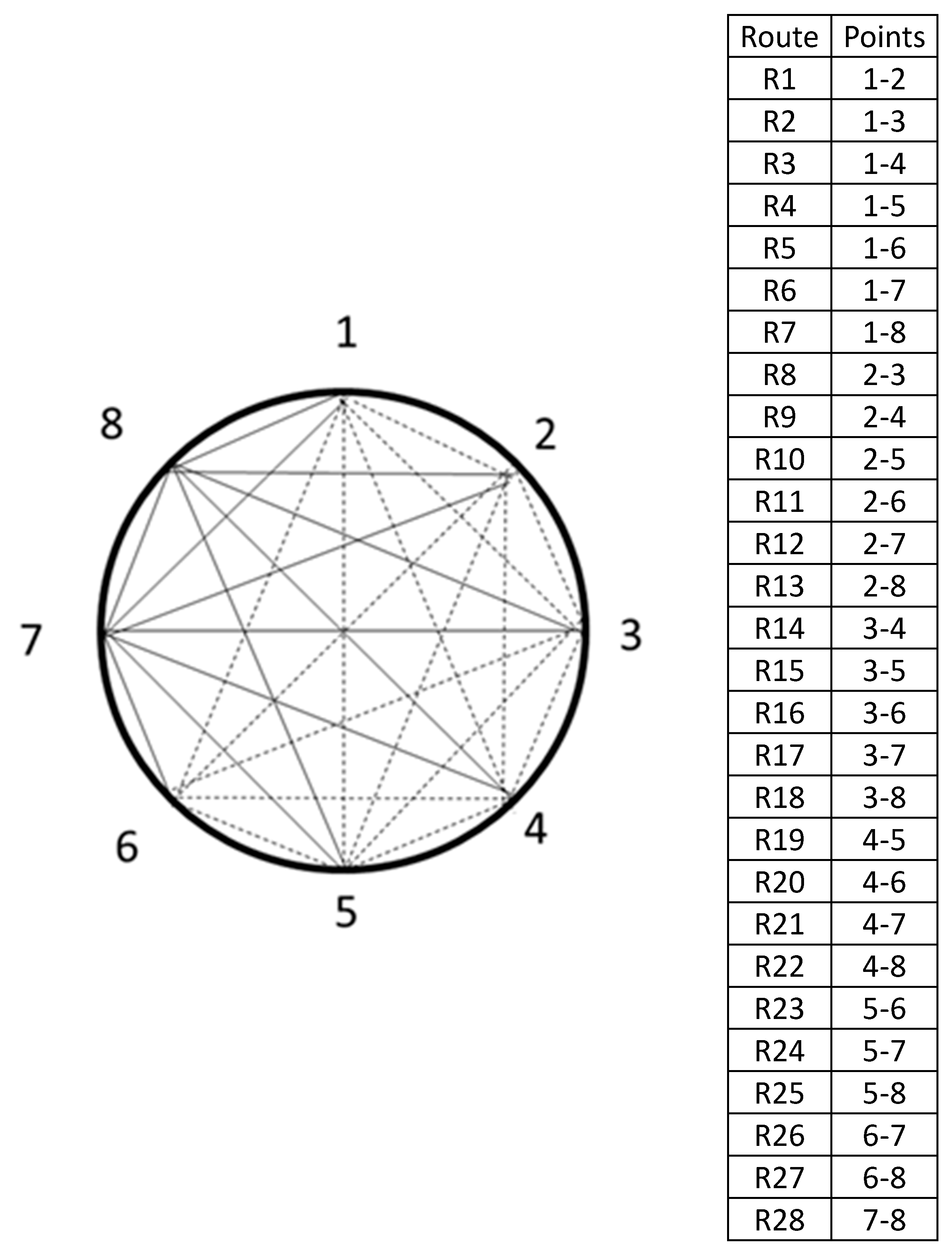
2.3.1. Tests
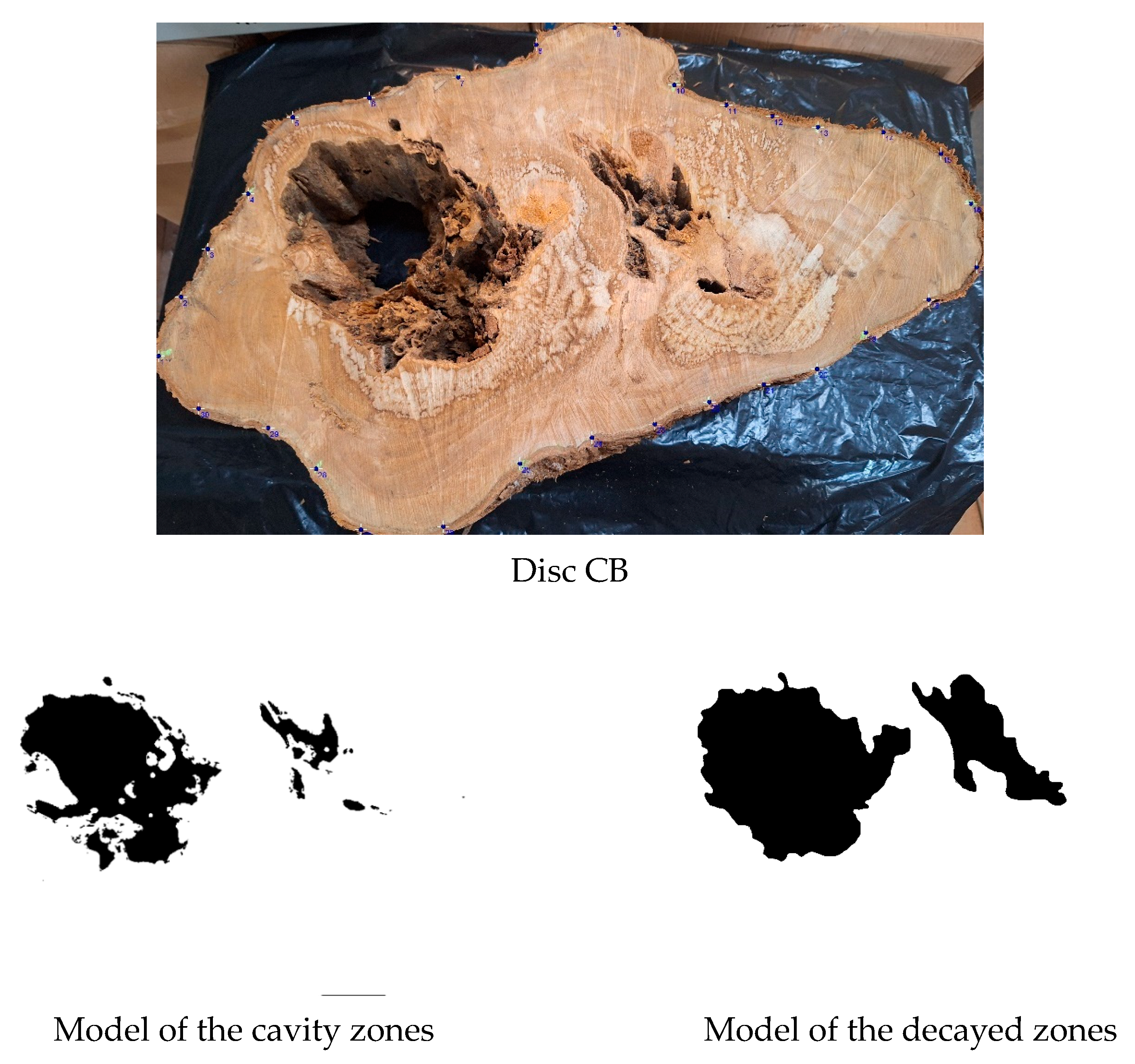
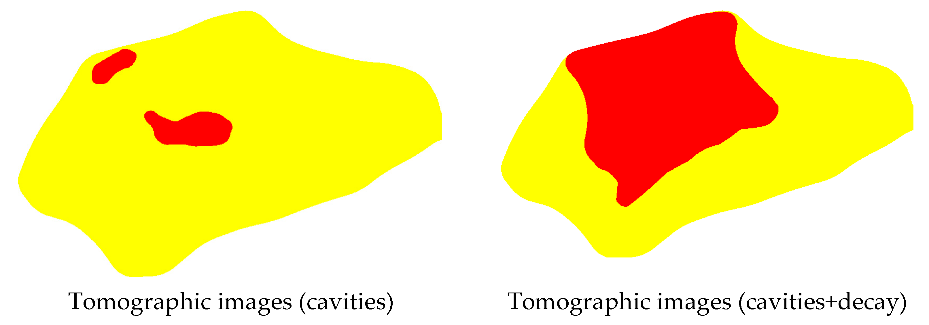
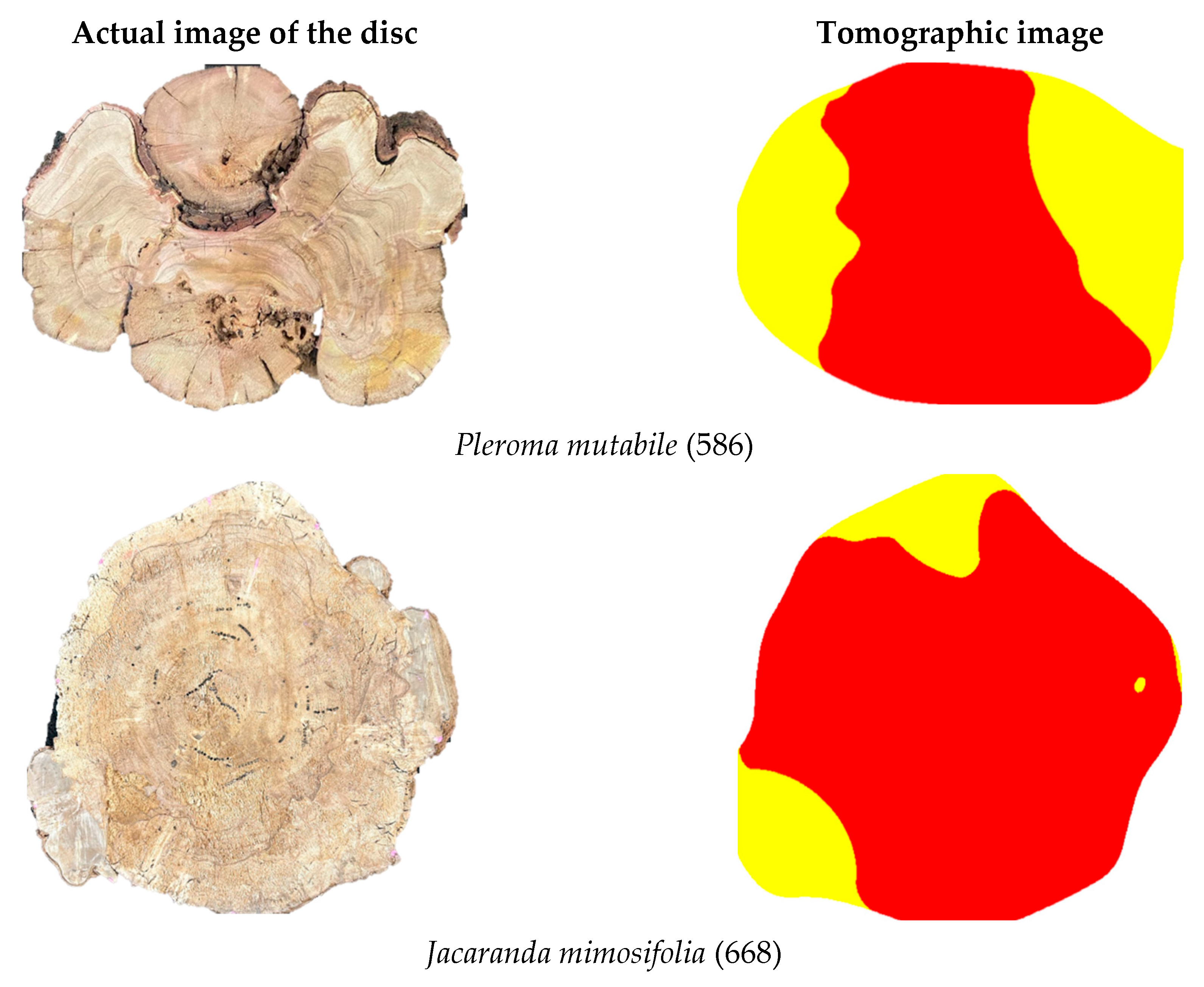
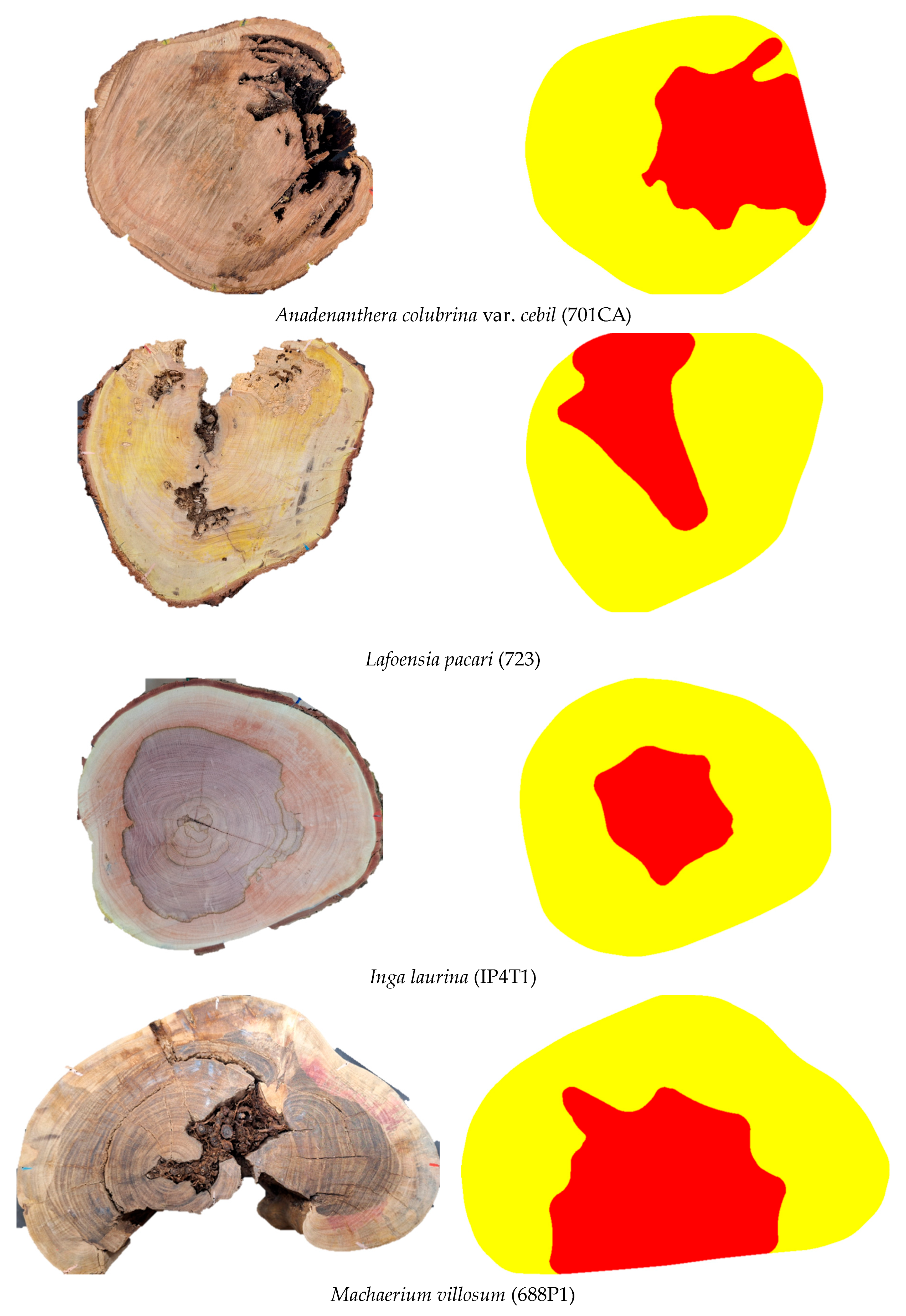
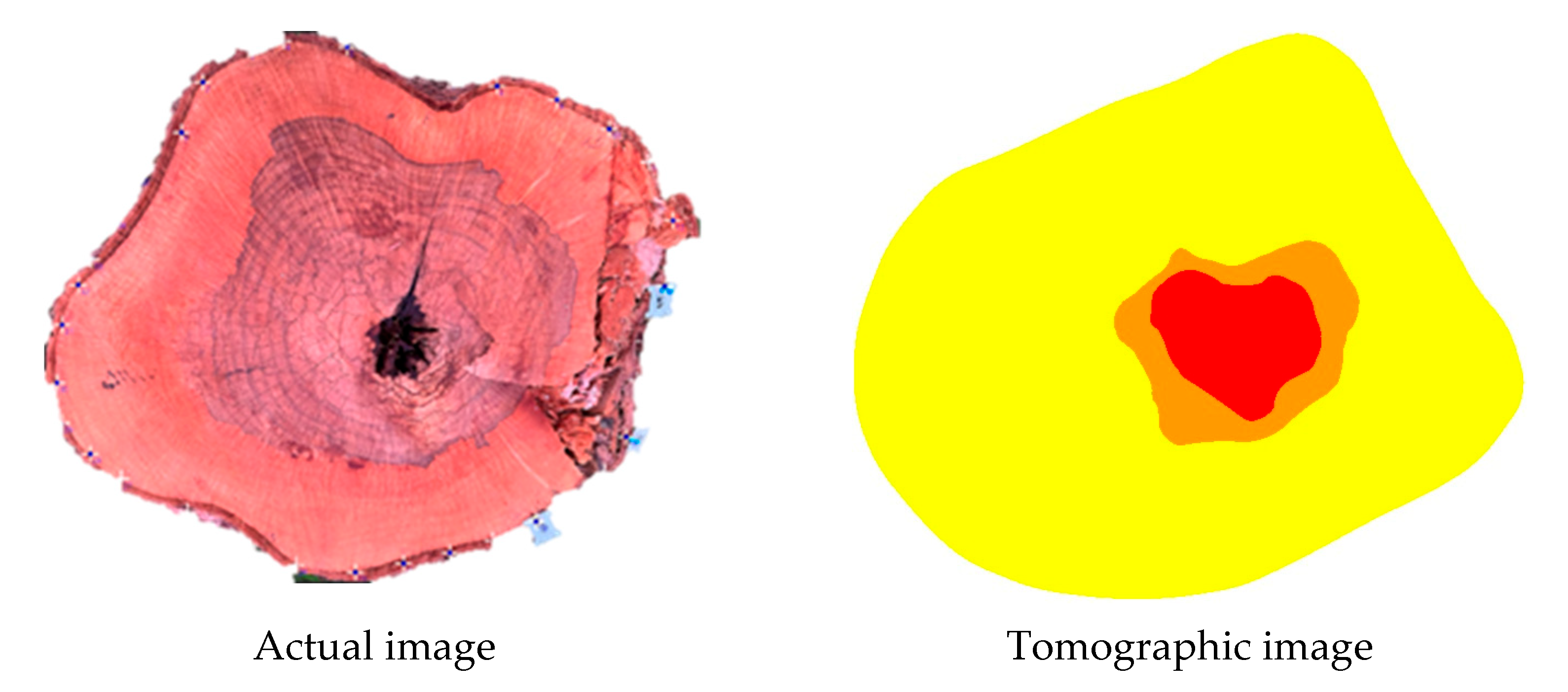
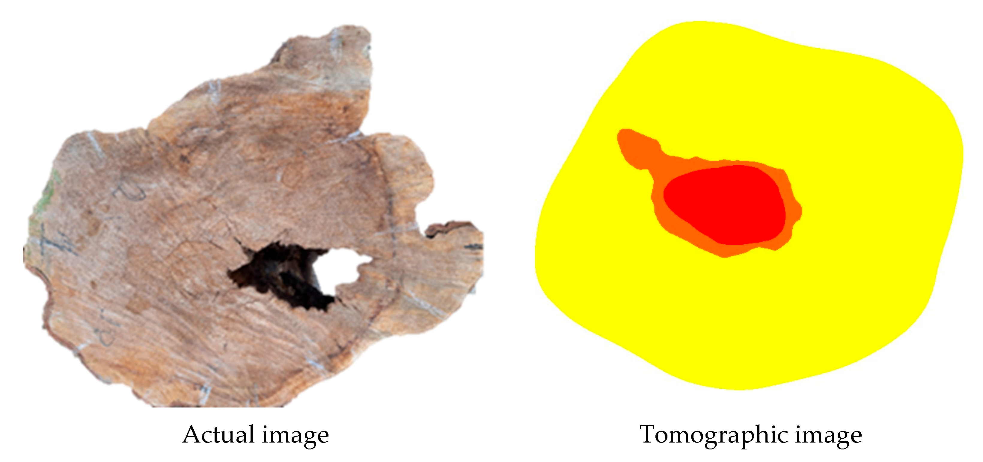
2.3.2. Tomographic Images
2.3.3. Confusion Matrix
Scale Adjustment
Model, ROI, and Internal Points Parameters
Accuracy Calculation
Evaluation of Results
3. Results
4. Discussion
5. Conclusions
- When the trunk is clean or with early stage decay the tomographic image generated using the proposed methodology accurately reflects this condition, showing no signs of deterioration regardless of the velocity thresholds interval adopted (35% to 50% of the maximum velocity). In this case the accuracy was 100%.
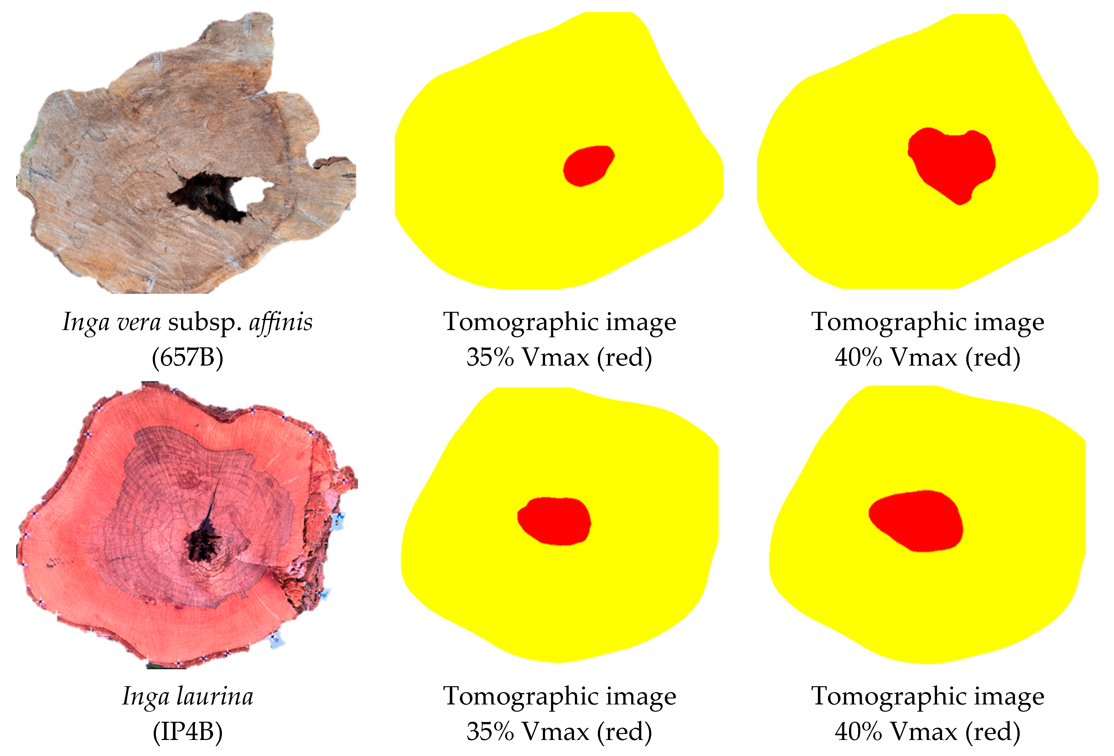
- For discs with isolated cavities (surrounded by clear wood or wood with early stage decay) the velocity thresholds intervals up to 35% Vmax show accuracy greater than 94%.
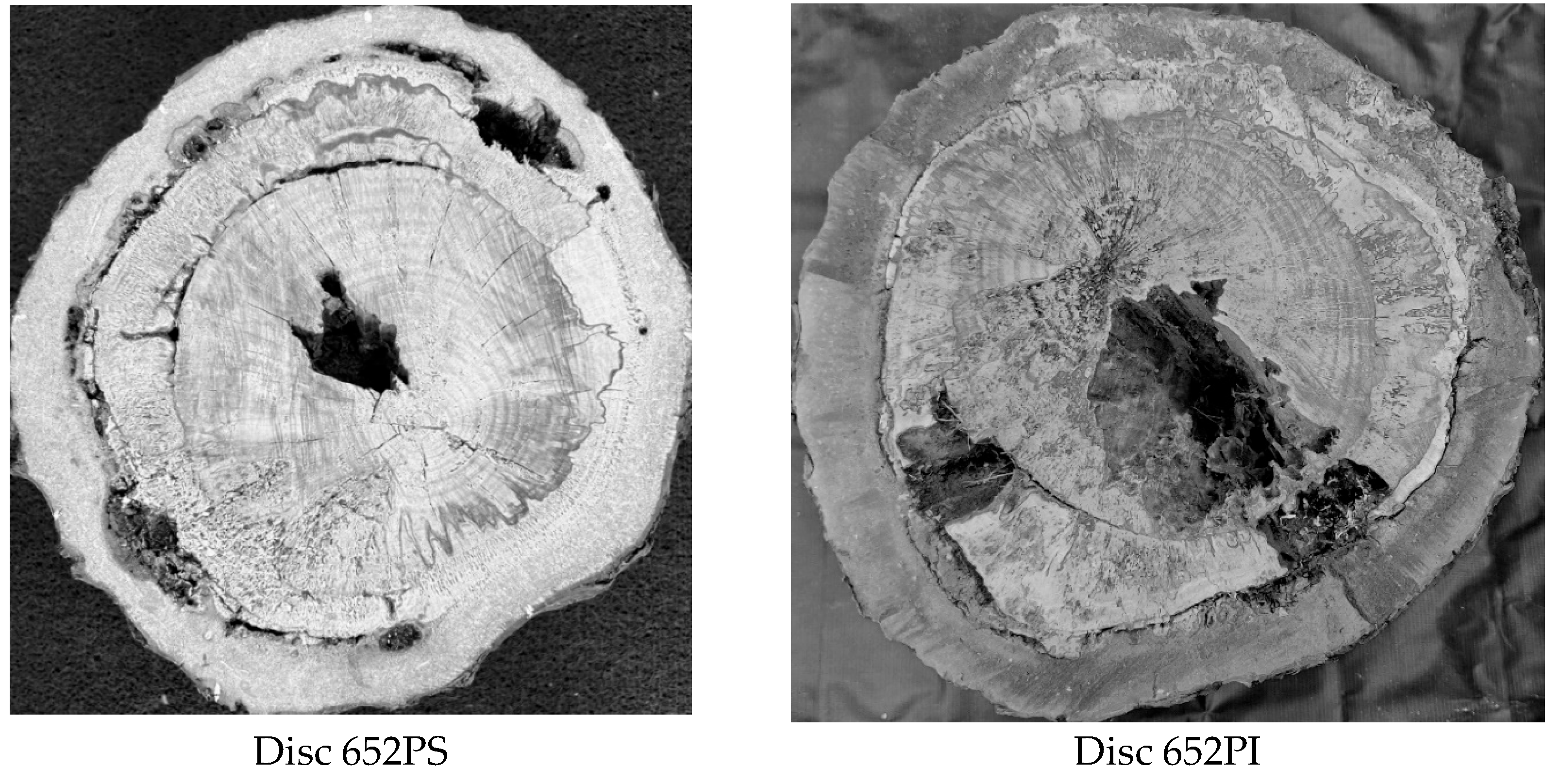
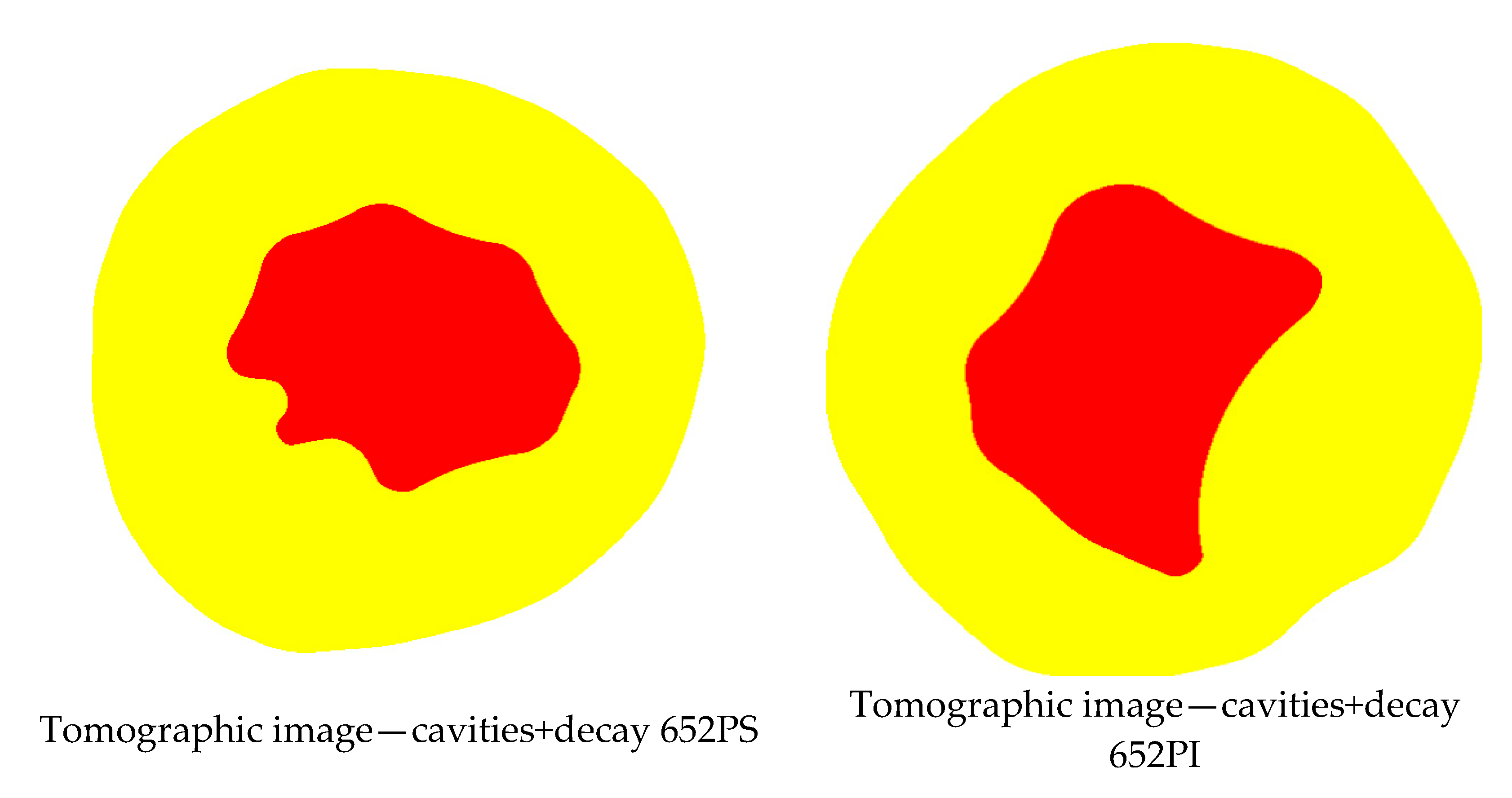
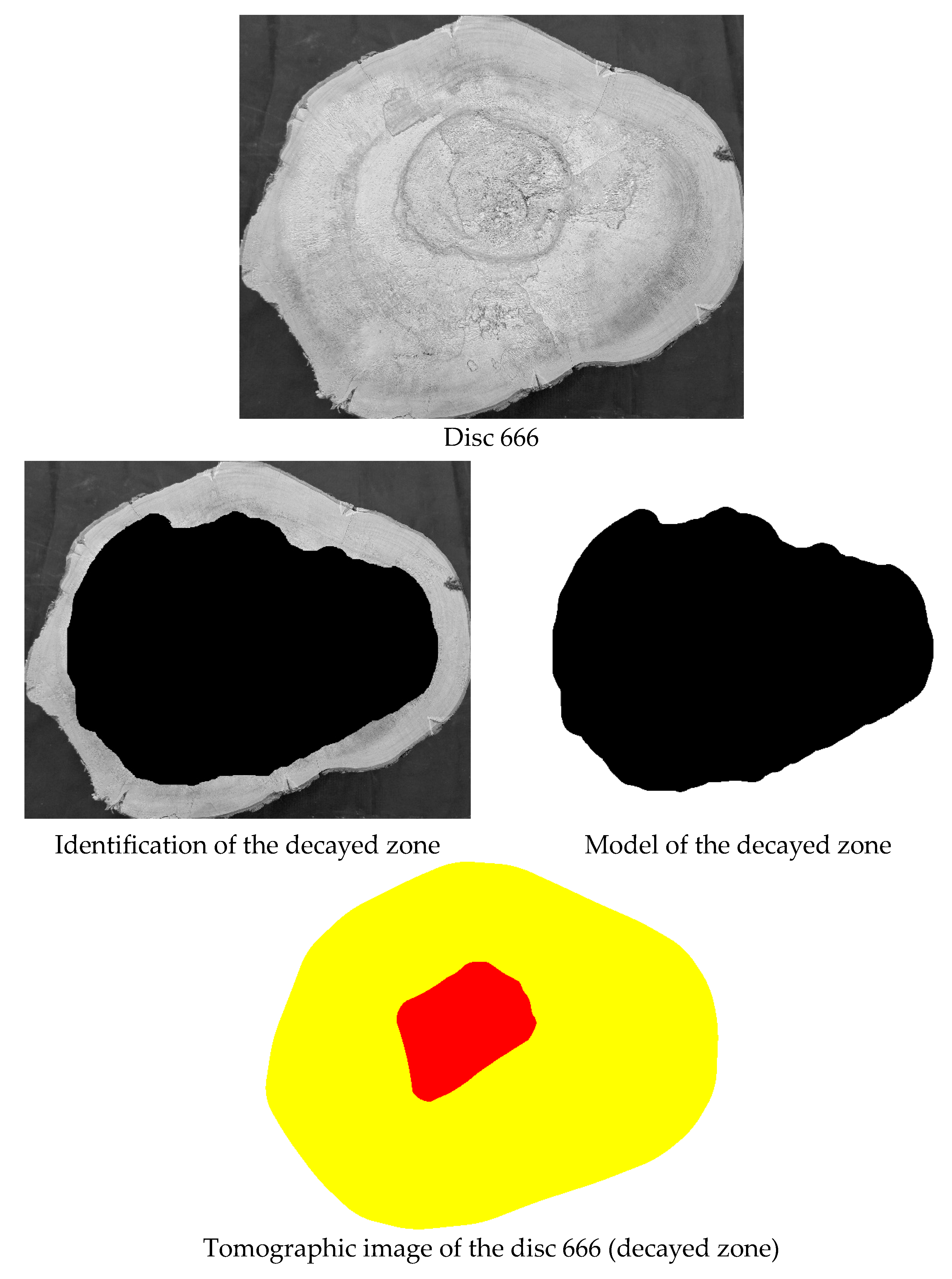
- For discs with cavities associated with decay the velocity thresholds intervals up to 35% Vmax can be adopted, independent of the species, to infer the cavity zone with good accuracy (84% on average). To infer the decayed zone the velocity threshold intervals up to 50%, also independent of the species, allow moderate accuracy (65% on average).
6. Patents
Author Contributions
Funding
Data Availability Statement
Acknowledgments
Conflicts of Interest
References
- Sankar Cheela, V.R.; Michele, J.; Wahidul, B.; Prabir, S. Combating Urban Heat Island Effect—A Review of Reflective Pavements and Tree Shading Strategies. Buildings 2021, 11, 93. [Google Scholar] [CrossRef]
- Liu, N.; Zhang, F. Urban green spaces and flood disaster management: Toward sustainable urban design. Front. Public Health 2025, 13, 1583978. [Google Scholar] [CrossRef] [PubMed]
- Chakraborty, T.; Biswas, T.; Campbell, L.S.; Franklin, B.; Parker, S.S.; Tukman, M. Feasibility of afforestation as an equitable nature-based solution in urban areas. Sustain. Cities Soc. 2022, 81, 103826. [Google Scholar] [CrossRef]
- Jones, B.A. Planting urban trees to improve quality of life? The life satisfaction impacts of urban afforestation. For. Policy Econ. 2021, 125, 102408. [Google Scholar] [CrossRef]
- Wolf, K.L.; Lam, S.T.; McKeen, J.K.; Richardson, G.R.A.; van den Bosch, M.; Bardekjian, A.C. Urban Trees and Human Health: A Scoping Review. Int. J. Environ. Res. 2020, 17, 4371. [Google Scholar] [CrossRef]
- Srivanit, M.; Kaewkhow, S. A machine learning-based protocol to support visual tree assessment and risk of failure classification on a university campus. Urban For. Urban Green. 2024, 99, 128420. [Google Scholar] [CrossRef]
- Hui, K.K.W.; Wong, M.S.; Kwok, C.Y.T.; Li, H.; Abbas, S.; Nichol, J.E. Unveiling falling urban trees before and during Typhoon Higos (2020): Empirical case study of potential structural failure using tilt sensor. Forests 2022, 13, 359. [Google Scholar] [CrossRef]
- Judice, A.; Gordon, J.; Abrams, J.; Irwin, K. Community perceptions of tree risk and management. Land 2021, 10, 1096. [Google Scholar] [CrossRef]
- Soge, A.O.; Popoola, O.I.; Adetoyinbo, A.A. Detection of wood decay and cavities in living trees: A review. Can. J. For. Res. 2021, 51, 937–947. [Google Scholar] [CrossRef]
- Li, H.; Zhang, X.; Li, Z.; Wen, J.; Tan, X. A review of research on tree risk assessment methods. Forests 2022, 13, 1556. [Google Scholar] [CrossRef]
- Coelho-Duarte, A.P.; Daniluk-Mosquera, G.; Gravina, V.; Vallejos-Barra, Ó.; Ponce-Donoso, M. Tree risk assessment: Component analysis of six visual methods applied in an urban park, Montevideo, Uruguay. Urban For. Urban Green. 2021, 59, 127005. [Google Scholar] [CrossRef]
- Klein, R.W.; Koeser, A.K.; Hauer, R.J.; Hansen, G.; Escobedo, F.J. Risk assessment and risk perception of trees: A review of literature relating to arboriculture and urban forestry. Arboric. Urban For. 2019, 45, 26–38. [Google Scholar] [CrossRef]
- Nicolotti, G.; Socco, L.V.; Martinis, R.; Godio, A.; Sambuelli, L. Application and comparison of three tomographic techniques for the detection of decay in trees. J. Arboric. 2003, 29, 66–78. [Google Scholar] [CrossRef]
- Wang, X.; Allison, R.B. Decay detection in red oak trees using a combination of visual inspection, acoustic testing, and resistance microdrilling. Arboric. Urban For. 2008, 34, 1–4. [Google Scholar] [CrossRef]
- Wang, X.; Wiedenbeck, J.; Liang, S. Acoustic tomography for decay detection in black cherry trees. Wood Fiber Sci. 2009, 41, 127–137. [Google Scholar]
- Palma, S.S.A.; Gonçalves, R. Tomographic images of tree trunks generated using ultrasound and post-processed images: Influence of the number of measurement points. BioResources 2022, 17, 6638–6655. [Google Scholar] [CrossRef]
- Palma, S.S.A.; Reis, M.N.; Gonçalves, R. Tomographic Images Generated from Measurements in Standing Trees Using Ultrasound and Postprocessed Images: Methodological Proposals for Cutting Velocity, Interpolation Algorithm and Confusion Matrix Metrics Focusing on Image Quality. Forests 2022, 13, 1935. [Google Scholar] [CrossRef]
- Wang, X.; Divos, F.; Pilon, C.; Brashaw, B.K.; Ross, R.J.; Pellerin, R.F. Assessment of Decay in Standing Timber Using Stress Wave Timing Nondestructive Evaluation Tools; USDA FS Forest Products Laboratory General Technical Report FPL-GTR-147; US Department of Agriculture Forest Service: Washington, DC, USA, 2004.
- Burcham, D.C.; Brazee, N.J.; Marra, R.E.; Kane, B. Geometry matters for sonic tomography of trees. Trees 2023, 37, 837–848. [Google Scholar] [CrossRef]
- Wei, X.; Xu, S.; Sun, L.; Tian, C.; Du, C. Propagation velocity model and two-dimensional defect imaging of stress wave in Larch (Larix gmelinii) wood. Bioresources 2021, 16, 6799–6813. [Google Scholar] [CrossRef]
- Yıldızcan, E.N.; Ari, M.E.; Tunga, B.; Gelir, A.; Kurul, F.; As, N.; Dündar, T. Machine learning based tomographic image reconstruction technique to detect hollows in wood. Wood Sci. Technol. 2024, 58, 1491–1516. [Google Scholar] [CrossRef]
- Ostrovský, R.; Kobza, M.; Gažo, J. Extensively damaged trees tested with acoustic tomography considering tree stability in urban greenery. Trees 2017, 31, 1015–1023. [Google Scholar] [CrossRef]
- Vieira-dos-Santos-Ataide, G.C.; dos-Santos-Ataide, D.H.; Cerqueira-Martins, B.; Monteiro-de-Carvalho, A.; de-Figueiredo-Latorraca, J.V. Historic urban trees: Assessing the trunk’s internal integrity. Bosque 2023, 44, 481–491. [Google Scholar] [CrossRef]
- Feng, H.; Li, G.; Fu, S.; Wang, X. Tomographic image reconstruction using an interpolation method for tree decay detection. BioResources 2014, 9, 3248–3263. [Google Scholar] [CrossRef]
- Strobel, J.R.A.; Carvalho, M.A.G.; Gonçalves, R.; Pedroso, C.B.; Reis, M.N.; Martins, P. Quantitative image analysis of acoustic tomography in woods. Eur. J. Wood Wood Prod. 2018, 76, 1379–1389. [Google Scholar] [CrossRef]
- Espinosa, L.; Prieto, F.; Brancheriau, L.; Lasaygues, P. Quantitative parametric imaging by ultrasound computed tomography of trees under anisotropic conditions: Numerical case study. Ultrasonics 2020, 102, 106060. [Google Scholar] [CrossRef] [PubMed]
- Wu, X.; Li, G.; Jiao, Z.; Wang, X. Reliability of acoustic tomography and ground-penetrating radar for tree decay detection. Appl. Plant Sci. 2018, 6, e01187. [Google Scholar] [CrossRef]
- Dudkiewicz, M.; Durlak, W. Sonic Tomograph as a tool supporting the sustainable management of historical greenery of the UMCS Botanical Garden in Lublin. Sustainability 2021, 13, 9451. [Google Scholar] [CrossRef]
- Michajlová, K.; Gejdoš, M.; Gergeľ, T.; Gretsch, D. Evaluation of the quality of standing trees using an Arbotom acoustic stress tomograph. For. J. 2025, 71, 65–72. [Google Scholar] [CrossRef]
- Du, X.; Li, J.; Feng, H.; Chen, S. Image reconstruction of internal defects in wood based on segmented propagation rays of stress waves. Appl. Sci. 2018, 8, 1778. [Google Scholar] [CrossRef]
- Kralovec, C.; Schagerl, M. Review of structural health monitoring methods regarding a multi-sensor approach for damage assessment of metal and composite structures. Sensors 2020, 20, 826. [Google Scholar] [CrossRef]
- Marcantonio, V.; Monarca, D.; Colantoni, A.; Cecchini, M. Ultrasonic waves for materials evaluation in fatigue, thermal and corrosion damage: A review. Mech. Syst. Signal Process. 2019, 120, 32–42. [Google Scholar] [CrossRef]
- Honarvar, F.; Varvani-Farahani, A. A review of ultrasonic testing applications in additive manufacturing: Defect evaluation, material characterization, and process control. Ultrasonics 2020, 108, 106227. [Google Scholar] [CrossRef] [PubMed]
- Bucur, V. Acoustics of Wood, 3rd ed.; Springer: Berlin/Heidelberg, Germany, 2025; 917p. [Google Scholar]
- Bucur, V. A review on acoustics of wood as a tool for quality assessment. Forests 2023, 14, 1545. [Google Scholar] [CrossRef]
- Espinosa, L.; Prieto, F.; Brancheriau, L.; Lasaygues, P. Effect of wood anisotropy in ultrasonic wave propagation: A ray-tracing approach. Ultrasonics 2019, 91, 242–251. [Google Scholar] [CrossRef]
- Perlin, L.P.; de Andrade Pinto, R.C.; do Valle, Â. Ultrasonic tomography in wood with anisotropy consideration. Constr. Build. Mater. 2019, 229, 116958. [Google Scholar] [CrossRef]
- Lorenzi, H. Árvores Brasileiras: Manual de Identificação e Cultivo de Plantas Arbóreas Nativas do Brasil, 6th ed.; Plantarum: Nova Odessa, Brazil, 2014; Volume 1, p. 384. [Google Scholar]
- Silva, H.F.; Ribeiro, S.C.; Botelho, S.A.; Faria, R.A.V.B.; Teixeira, M.B.R.; Mello, J.M. Estimativa do estoque de carbono por métodos indiretos em área de restauração florestal em Minas Gerais. Sci. For. 2015, 43, 943–953. [Google Scholar] [CrossRef]
- Vale, A.; Sarmento, T.R.; Almeida, A.N. Caracterização e uso de madeiras de galhos de árvores provenientes da arborização de Brasília, DF. Ciênc. Florest. 2005, 15, 33–42. [Google Scholar] [CrossRef]
- Britez, R.M.; Borgo, M.; Tiepolo, G.; Ferretti, A.; Calmon, M.; Higa, R.C.V. Estoque e Incremento de Carbono em Florestas e Povoamentos de Espécies Arbóreas com Ênfase na Floresta Atlântica do Sul do Brasil; Embrapa Florestas: Colombo, Brazil, 2006; ISBN 85-89281-07-8. [Google Scholar]
- Restor. Biodiversity—Trees. Restor. Available online: https://restor.eco/pt/platform/sites/13831d32-d1c0-40f7-abe4-ed23d3d273f7/biodiversity/trees/ (accessed on 23 May 2025).
- Gonçalves, M.T.T. Contribuição para o Estudo da Usinagem de Madeiras. Master’s Dissertation, Escola de Engenharia de São Carlos, Universidade de São Paulo, São Carlos, Brazil, 1990. [Google Scholar] [CrossRef]
- Suryawanshi, M.; Patel, A.; Kale, T.; Patil, P. Carbon sequestration potential of tree species in the environment of North Maharashtra University Campus, Jalgaon (MS), India. Biosci. Discov. 2014, 5, 175–179. [Google Scholar]
- Du, X.; Li, S.; Li, G.; Feng, H.; Chen, S. Stress wave tomography of wood internal defects using ellipse-based spatial interpolation and velocity compensation. BioResources 2015, 10, 3948–3962. [Google Scholar] [CrossRef]
- Schubert, S.; Gsell, D.; Dual, J.; Motavalli, M.; Niemz, P. Acoustic wood tomography on trees and the challenge of wood heterogeneity. Holzforschung 2009, 63, 107–112. [Google Scholar] [CrossRef]
- Danielli, D. Densidade da Madeira e Potencial Dendrocronológico de Espéceis Nativas da Floresta Ombrófila Mista (Wood Density and Dendrochronological Potential of Native Species from Mixed Ombrophilous Forest). Master’s Dissertation, State University of Santa Catarina, Florianópolis, Brazil, 2017; p. 115. [Google Scholar]


| Botanical Classification of Tree Species | Basic Density (kg/m3) | Discs | ||
|---|---|---|---|---|
| Botanical Family | Scientific Name | Sound | Defective | |
| Araucariaceae * | Araucaria angustifolia (Bertol.) Kuntze | 550 [38] | 0 | 2 |
| Anacardiaceae | Lithraea molleoides (Vell.) Engl. | 610 [39] | 0 | 1 |
| Anacardiaceae | Mangifera indica L. | 520 [40] | 2 | 0 |
| Bignoniaceae | Jacaranda mimosifolia D. Don | 600 [41] | 6 | 2 ** |
| Bignoniaceae | Sparattosperma leucanthum (Vell.) K.Schum. | 570 [38] | 0 | 1 |
| Fabaceae | Amburana cearensis (Allemão) A.C.Sm. | 600 [38] | 1 | 0 |
| Fabaceae | Anadenanthera colubrina var. cebil (Griseb.) Altschul | 1005 [38] | 0 | 3 |
| Fabaceae | Dalbergia nigra (Vell.) Allemão ex Benth. | 870 [40] | 1 | 0 |
| Fabaceae | Delonix regia (Bojer ex Hook.) Raf. | 510 [40] | 1 | 0 |
| Fabaceae | Entada abyssinica Steud. ex A.Rich. | 540 [42] | 3 | 0 |
| Fabaceae | Inga laurina (Sw.) Willd. | 710 [38] | 0 | 3 |
| Fabaceae | Inga vera subsp. Affinis (DC.) T.D.Penn. | 580 [38] | 0 | 1 |
| Fabaceae | Machaerium villosum Vogel | 850 [38] | 0 | 2 |
| Fabaceae | Poecilanthe parviflora Benth. | 990 [38] | 1 | 0 |
| Fabaceae | Samanea tubulosa (Benth.) Barneby & J.W.Grimes | 780 [38] | 1 | 0 |
| Lythraceae | Lafoensia pacari A.St.-Hil. | 800 [38] | 0 | 1 |
| Melastomataceae | Pleroma mutabile (Vell.) Triana | 660 [38] | 0 | 1 |
| Meliaceae | Swietenia mahagoni (L.) Jacq. | 590 [43] | 1 | 0 |
| Oleaceae | Ligustrum lucidum W.T.Aiton | 560 [40] | 0 | 1 |
| Polygonaceae | Triplaris americana L. | 450 [44] | 0 | 1 |
| Proteaceae | Grevillea robusta A.Cunn. ex R.Br. | 560 [43] | 2 | 0 |
| Total | 19 | 19 | ||
| Scientific Names | Disc ID | Perimeter (m) | Number of Diffraction Mesh Points |
|---|---|---|---|
| Araucaria angustifolia | 652PS | 1.05 | 8 |
| 652PI | 1.10 | 8 | |
| Lithraea molleoides | 633 | 1.25 | 8 |
| Mangifera indica | 595 | 0.98 | 8 |
| MSN2024 | 1.98 | 10 | |
| Jacaranda mimosifolia | 654 | 0.82 | 8 |
| 666 | 1.24 | 8 | |
| 667 | 1.06 | 8 | |
| 668 | 2.04 | 10 | |
| 669 | 1.84 | 10 | |
| 670 | 1.71 | 8 | |
| 671 | 1.41 | 8 | |
| 672 | 1.19 | 8 | |
| Sparattosperma leucanthum | CB1 | 1.94 | 10 |
| Amburana cearensis | 668 | 1.22 | 8 |
| Anadenanthera colubrina var. cebil | 701CF | 1.18 | 8 |
| 701CA | 1.21 | 8 | |
| 702 | 1.02 | 8 | |
| Dalbergia nigra | 656 | 1.31 | 8 |
| Delonix regia | 682 | 1.46 | 8 |
| Entada abyssinica | 678 | 1.23 | 8 |
| 678SN | 1.19 | 8 | |
| 679 | 1.00 | 8 | |
| Inga laurina | IP4T1 | 1.45 | 12 |
| IP4B | 2.30 | 8 | |
| IP4T1L | 1.34 | 8 | |
| Inga vera subsp. affinis | 657B | 1.95 | 10 |
| Machaerium villosum | 688P1 | 0.96 | 8 |
| 688P2 | 1.00 | 8 | |
| Poecilanthe parviflora | 636 | 1.14 | 8 |
| Samanea tubulosa | 653 | 1.11 | 8 |
| Lafoensia pacari | 723 | 1.10 | 8 |
| Pleroma mutabile | 586 | 1.18 | 8 |
| Swietenia mahagoni | 572 | 1.36 | 8 |
| Ligustrum lucidum | 582 | 1.37 | 8 |
| Triplaris americana | 593 | 1.05 | 8 |
| Grevillea robusta | 607 | 0.90 | 8 |
| 608 | 0.80 | 8 |
| Scientific Names | Discs ID | Acuracy (%) | |||
|---|---|---|---|---|---|
| 35% Vmax | 40% Vmax | 45% Vmax | 50% Vmax | ||
| Araucaria angustifolia | 652PS | 71 | 72 | 67 | 64 |
| 652PI | 88 | 89 | 83 | 78 | |
| Lithraea molleoides | 633 | 73 | 68 | 63 | 59 |
| Mangifera indica | 595 | 100 | 100 | 100 | 100 |
| MSN2024 | 100 | 100 | 100 | 100 | |
| Jacaranda mimosifolia | 654 | 100 | 100 | 100 | 100 |
| 666 | 100 | 100 | 100 | 100 | |
| 667 | 100 | 100 | 100 | 100 | |
| 668 | 82 | 49 | 28 | 15 | |
| 669 | 100 | 100 | 100 | 100 | |
| 670 | 100 | 100 | 100 | 100 | |
| 671 | 100 | 100 | 100 | 100 | |
| 672 | 100 | 100 | 100 | 100 | |
| Sparattosperma leucanthum | CB1 | 85 | 88 | 85 | 73 |
| Amburana cearensis | 668 | 100 | 100 | 100 | 100 |
| Anadenanthera colubrina var. cebil | 701CF | 83 | 81 | 79 | 75 |
| 701CA | 83 | 81 | 78 | 75 | |
| 702 | 93 | 86 | 79 | 72 | |
| Dalbergia nigra | 656 | 100 | 100 | 100 | 100 |
| Delonix regia | 682 | 100 | 100 | 100 | 100 |
| Entada abyssinica | 678 | 100 | 100 | 100 | 100 |
| 678SN | 100 | 100 | 100 | 100 | |
| 679 | 100 | 100 | 100 | 100 | |
| Inga laurina | IP4T1 | 81 | 80 | 69 | 52 |
| IP4B | 95 | 93 | 87 | 79 | |
| IP4T1L | 92 | 83 | 67 | 57 | |
| Inga vera subsp. affinis | 657B | 94 | 91 | 89 | 83 |
| Machaerium villosum | 688P1 | 88 | 83 | 73 | 66 |
| 688P2 | 83 | 79 | 71 | 68 | |
| Poecilanthe parviflora | 636 | 100 | 100 | 100 | 100 |
| Samanea tubulosa | 653 | 100 | 100 | 100 | 100 |
| Lafoensia pacari | 723 | 83 | 76 | 70 | 68 |
| Pleroma mutabile | 586 | 72 | 66 | 54 | 42 |
| Swietenia mahagoni | 572 | 100 | 100 | 100 | 100 |
| Ligustrum lucidum | 582 | 71 | 72 | 67 | 64 |
| Triplaris americana | 593 | 96 | 95 | 92 | 88 |
| Grevillea robusta | 607 | 100 | 100 | 100 | 100 |
| 608 | 100 | 100 | 100 | 100 | |
| Scientific Names | Discs ID | Acuracy (%) | |||
|---|---|---|---|---|---|
| 35% Vmax | 40% Vmax | 45% Vmax | 50% Vmax | ||
| Araucaria angustifolia | 652PS | 50 | 52 | 54 | 56 |
| 652PI | 31 | 36 | 45 | 54 | |
| Lithraea molleoides | 633 | 50 | 58 | 64 | 65 |
| Mangifera indica | 595 | 100 | 100 | 100 | 100 |
| MSN2024 | 100 | 100 | 100 | 100 | |
| Jacaranda mimosifolia | 654 | 100 | 100 | 100 | 100 |
| 666 | 0 | 35 | 37 | 44 | |
| 667 | 100 | 100 | 100 | 100 | |
| 668 | 28 | 59 | 78 | 86 | |
| 669 | 100 | 100 | 100 | 100 | |
| 670 | 100 | 100 | 100 | 100 | |
| 671 | 100 | 100 | 100 | 100 | |
| 672 | 100 | 100 | 100 | 100 | |
| Sparattosperma leucanthum | CB1 | 78 | 84 | 84 | 78 |
| Amburana cearensis | 668 | 100 | 100 | 100 | 100 |
| Anadenanthera colubrina var. cebil | 701CF | 56 | 58 | 61 | 59 |
| 701CA | 70 | 71 | 73 | 75 | |
| 702 | 77 | 73 | 68 | 63 | |
| Dalbergia nigra | 656 | 100 | 100 | 100 | 100 |
| Delonix regia | 682 | 100 | 100 | 100 | 100 |
| Entada abyssinica | 678 | 100 | 100 | 100 | 100 |
| 678SN | 100 | 100 | 100 | 100 | |
| 679 | 100 | 100 | 100 | 100 | |
| IP4T1L | 66 | 70 | 71 | 71 | |
| Inga laurina | IP4T1 | 56 | 56 | 55 | 48 |
| IP4B | 60 | 63 | 66 | 71 | |
| Inga vera subsp. affinis | 657B | 81 | 80 | 80 | 76 |
| Machaerium villosum | 688P1 | 75 | 80 | 83 | 83 |
| 688P2 | 61 | 61 | 58 | 57 | |
| Poecilanthe parviflora | 636 | 100 | 100 | 100 | 100 |
| Samanea tubulosa | 653 | 100 | 100 | 100 | 100 |
| Lafoensia pacari | 723 | 74 | 69 | 65 | 64 |
| Pleroma mutabile | 586 | 40 | 48 | 58 | 67 |
| Swietenia mahagoni | 572 | 100 | 100 | 100 | 100 |
| Ligustrum lucidum | 582 | 73 | 75 | 72 | 72 |
| Triplaris americana | 593 | 49 | 48 | 45 | 43 |
| Grevillea robusta | 607 | 100 | 100 | 100 | 100 |
| 608 | 100 | 100 | 100 | 100 | |
Disclaimer/Publisher’s Note: The statements, opinions and data contained in all publications are solely those of the individual author(s) and contributor(s) and not of MDPI and/or the editor(s). MDPI and/or the editor(s) disclaim responsibility for any injury to people or property resulting from any ideas, methods, instructions or products referred to in the content. |
© 2025 by the authors. Licensee MDPI, Basel, Switzerland. This article is an open access article distributed under the terms and conditions of the Creative Commons Attribution (CC BY) license (https://creativecommons.org/licenses/by/4.0/).
Share and Cite
Volpi, L.T.; Palma, S.S.A.; Gonçalves, R. Velocity Thresholds for Ultrasonic Tomographic Imaging Aimed at Detecting Cavities and Decay in Trees. Forests 2025, 16, 995. https://doi.org/10.3390/f16060995
Volpi LT, Palma SSA, Gonçalves R. Velocity Thresholds for Ultrasonic Tomographic Imaging Aimed at Detecting Cavities and Decay in Trees. Forests. 2025; 16(6):995. https://doi.org/10.3390/f16060995
Chicago/Turabian StyleVolpi, Larissa Tiago, Stella Stopa Assis Palma, and Raquel Gonçalves. 2025. "Velocity Thresholds for Ultrasonic Tomographic Imaging Aimed at Detecting Cavities and Decay in Trees" Forests 16, no. 6: 995. https://doi.org/10.3390/f16060995
APA StyleVolpi, L. T., Palma, S. S. A., & Gonçalves, R. (2025). Velocity Thresholds for Ultrasonic Tomographic Imaging Aimed at Detecting Cavities and Decay in Trees. Forests, 16(6), 995. https://doi.org/10.3390/f16060995