Article

Developing Diameter Distribution Models of Major Coniferous Species in South Korea

1
Department of Forest Management, College of Forest and Environmental Sciences, Kangwon National University, Chuncheon 24341, Republic of Korea
2
Natural Resources Institute Finland (Luke), Latokartanonkaari 9, 00790 Helsinki, Finland
*
Author to whom correspondence should be addressed.
Forests 2025, 16(6), 961; https://doi.org/10.3390/f16060961
Submission received: 25 February 2025 / Revised: 14 April 2025 / Accepted: 4 June 2025 / Published: 6 June 2025
(This article belongs to the Special Issue Silviculture and Management Strategy in Coniferous Forests)

Abstract

:
This study developed diameter distribution models using the Weibull function for Korean red pine (Pinus densiflora), Korean white pine (P. koraiensis), and Japanese larch (Larix kaempferi). The study data were collected from 49 Korean red pine stands, 54 Korean white pine stands, and 49 Japanese larch stands located in national forests in Gangwon and North Gyeongsang Provinces, South Korea. To identify the optimal method for modeling the diameter distribution of these three species, parameter recovery methods and parameter prediction methods were analyzed. To identify the optimal parameter recovery method for presenting the diameter distribution of these three species, ten parameter recovery methods were compared using moment-based, percentile-based, and hybrid approaches. For parameter prediction methods, major stand characteristics were used as independent variables to develop the models for the parameters a, b, and c of the Weibull function. For estimating the Weibull parameters, two methods—the estimated parameter recovery method and the parameter prediction method—were compared and analyzed. The optimal parameter recovery method was the one using the minimum DBH, the mean DBH, and the DBH variance. The coefficient of determination (R2) for the models predicting the minimum DBH, the mean DBH, and the DBH variance ranged from 0.7186 to 0.9747, and the R2 for the models directly predicting parameters ranged from 0.7032 to 0.9374, indicating high explanatory power and unbiased results. When comparing the two methods, the parameter prediction method showed higher accuracy and lower bias. In addition, paired t-tests were conducted to assess differences from the observed Weibull parameters. The results showed a significant difference for the estimated parameter recovery method, whereas no significant difference was found for the parameter prediction method, further supporting its reliability.

1. Introduction

Diameter distribution is one of the most fundamental and essential pieces of information in forest management, where growth characteristics at the stand level should be considered along with individual tree diameter growth to establish a silvicultural system [1]. In particular, information on diameter distribution is essential for predicting essential factors in the forest management decision-making process, such as thinning intensity and timing or predicted yield [2,3]. Additionally, diameter distribution is an essential factor in the timber industry, affecting decisions regarding timber price and quality, forest machinery types, production costs, and work methods during harvesting [4].
Korea Forest Service (KFS) has emphasized the cultivation of economic forests as a strategy to revitalize the forestry industry and create forestry-related jobs [5]. KFS aims to increase the annual production of domestic timber from 4.91 million m3 in 2015 to 8.61 million m3 by 2030. In line with this goal, KFS sought to establish a sustainable timber production system and increase the ratio of wood self-supply from 16.2% in 2016 to 30.0% by 2037, focusing on commercial forest development complexes.
Additionally, as “forests and trees” have been highlighted internationally as a solution against the climate crisis, Korea aims to enhance the role of forests as the key carbon sinks [6]. In particular, efforts are underway to expand the production of sawtimber, which is recognized under the IPCC standards as having a carbon storage period of over 50 years, thereby contributing to carbon absorption [5]. Consequently, the importance of producing domestic timber and large-diameter logs has become more pronounced, increasing the need for a rational forest silviculture system and precise data on diameter distribution characteristics.
In advanced forestry countries, studies on developing diameter distribution models using stand growth models and the Weibull function have been conducted to predict diameter growth [7,8,9]. In particular, Poudel and Cao [10] compared ten parameter recovery methods to select the optimal parameter recovery method and developed a diameter distribution model suitable for loblolly pine. In the study by Siipilehto and Mehtätalo [7], the parameter recovery method and the parameter prediction method were compared to determine which approach was more appropriate for estimating the Weibull parameters in Scots pine stands. These models are highly applicable for predicting diameter distribution and estimating yield using stand variables such as age and the number of stems [10,11,12]. Despite high applicability in forestry, studies on developing diameter distribution models in South Korea are insufficient. Therefore, as demonstrated in previous studies, comparing various methodological approaches—the parameter recovery method and the parameter prediction method—in the development of diameter distribution models enables more precise predictions, which can support rational decision-making in forest management [7].
Meanwhile, Korean red pine (Pinus densiflora; Pd), Korean white pine (P. koraiensis; Pk), and Japanese larch (Larix kaempferi; Lk) are the major coniferous species in South Korea, covering 1.991 million hectares, which accounts for 85.9% of the total coniferous forest area in the country [13]. These species are highly economically valuable for timber production, and the importance of the domestic timber supply and utilization is expected to increase [14,15,16]. Consequently, interest is increasing in how to manage these species to enhance timber production. In addition, the demand for diameter distribution information is increasing to estimate the production of large-diameter timber and yield in Korean red pine, Korean white pine, and Japanese larch stands.
This study was conducted to develop diameter distribution models using the Weibull function, focusing on plantations of Korean red pine, Korean white pine, and Japanese larch, which are major coniferous species in Korea. This study compared ten parameter recovery methods to select the optimal parameter recovery method for modeling the diameter distribution of major coniferous species in Korea. Additionally, the estimated parameter recovery method and the parameter prediction method were compared to determine the proper approach for estimating the Weibull parameters.

2. Materials and Methods

2.1. Data

This study was conducted in pure plantations of Korean red pine, Korean white pine, and Japanese larch within national forests managed by the Northern, Eastern, and Southern Regional Forest Services (Figure 1). Experimental sites are located between the 36°33′9.40″ N and 38°18′40.50″ N latitudes and between the 127°34′17.50″ E and 129°22′7.05″ E longitudes [17]. The sites are within Gangwon Province and North Gyeongsang Province in South Korea. A total of 147 Korean red pine sites, 162 Korean white pine sites, and 147 Japanese larch sites were included in the study. Each site consists of 3 plots: a non-thinning plot, a light thinning plot, and a heavy thinning plot. The plot sizes are 20 m × 20 m for the non-thinning plot, 25 m × 25 m for the light thinning plot, and 30 m × 30 m for the heavy thinning plot. Thinning intensity, based on the basal area, ranged from 0% to 59.8% across the sites and was designed to represent various stand densities [18]. The plots were designed to maintain similar stand characteristics, including stand density, species composition, aspect, and slope, to ensure stand homogeneity [19]. Plots exhibiting abnormal stand structure due to wind damage, forest fires, or other disturbances were excluded from the dataset. In this study, a total of 411 Korean red pine, 554 Korean white pine, and 537 Japanese larch cases were used at the plot level.
The inventory for data collection was conducted at 3-year intervals starting in 2012, with a maximum of 5 repeated inventories up to 2024. Trees planted within the plot were inventoried, and data were collected on variables including species, DBH, age, and height. DBH was measured at a height of 1.2 m from the ground using a D-tape. Age data were collected by conducting stem analysis on sample trees within the same stand as the experimental site [1,18,19]. Tree height was measured using a Haglöf Vertex IV. Summary statistics for the data collected through 2024 are shown in Table 1.

2.2. Modeling Approach and Statistical Analysis

2.2.1. Weibull Function

To develop the diameter distribution model, the Weibull function was used, as it is known from previous studies to best represent the diameter distribution [9,10,20,21]. The Weibull function is shown in Equation (1):
f x = c b ( x a b ) c 1 e x p ( x a b ) c
where a, b, and c are parameters of the Weibull function and x is the diameter at breast height (cm).
The Weibull function consists of three parameters. Parameter a is the location parameter, representing the minimum value of the distribution; no trees have a DBH smaller than this value. Parameter b is the scale parameter, which indicates the range of the diameter distribution. When parameter b is smaller, the distribution skews toward small-diameter trees, while a larger value indicates a higher proportion of large-diameter trees. Lastly, parameter c is the shape parameter. As parameter c increases, the diameter distribution becomes more concentrated around a specific diameter class. The shape of the distribution varies significantly with changes in parameter c [22,23].
To calculate the proportion of stems by diameter class within a stand, the upper and lower limits of each diameter class are substituted into Equation (2). Then, the value at the upper limit is subtracted from the value at the lower limit in the cumulative distribution function to determine the relative proportion of stems in each diameter class [1,24].
P i = 1 exp U i a b c ( 1 exp U i 1 a b c )
where exp() is the base of the natural logarithm; U i is the upper limit of DBH class i; and a, b, and c are parameters of the Weibull function.

2.2.2. Parameter Recovery Method

To find the best parameter recovery method for modeling diameter distributions, Weibull parameters were recovered using ten different methods (Table 2), and a method was selected to obtain the observed Weibull parameters for developing the final diameter distribution model for Korean red pine, Korean white pine, and Japanese larch stands.
The moment-based parameter recovery method (Methods 1 and 2) utilizes diameter moments to estimate the parameters of the Weibull distribution. This approach employs predicted values such as mean diameter, quadratic mean diameter, basal area, volume, and diameter variance to derive the Weibull parameters. Numerous previous studies applied this method [25,26,27].
The percentile-based parameter recovery method (Methods 3–9) utilizes regression models to estimate specific percentiles as functions of stand attributes, including age, site index, and stand density [10,28]. These predicted percentiles are subsequently used to calculate the parameters of the distribution. A key benefit of this approach is that characteristics of the diameter distribution, such as minimum diameter or specific percentiles, can often be estimated with greater accuracy than the parameters themselves [29]. This method, relying on different diameter percentiles, has been employed across various types of stands. The hybrid method (Method 10) combines the use of both moments and percentiles to recover distribution parameters. McTague and Bailey [30] introduced a technique that derives the Weibull parameters using the 10th, 63rd, and 93rd percentiles. This approach has been widely utilized in various studies [31,32,33,34]. The formulas for the moment-based parameter recovery method, the percentile-based parameter recovery method, and the hybrid method applied in this study were adopted based on previous studies [9,10,28,35].
To evaluate the goodness-of-fit when selecting the best parameter recovery method, the mean bias, the mean absolute error (MAE), the root mean square error (RMSE), the Kolmogorov–Smirnov statistic, and the error index (EI) were used. The formulas for calculating bias, the MAE, and the RMSE are provided in Equations (3)–(6):
B i a s = i = 1 n ( y i y ^ i ) n
M A E = i = 1 n y i y ^ i n
M S E = i = 1 n ( y i y ^ i ) 2 n
R M S E = i = 1 n ( y i y ^ i ) 2 n
where n is the number of plots; yi is the observed value of the sample i; and ŷi is the predicted value of the sample i.
The Kolmogorov–Smirnov (KS) test was used to evaluate the diameter distribution predicted from the recovered Weibull parameters. KS is a statistic used to assess the difference between two distributions by calculating the maximum absolute difference between the observed cumulative distribution function and the predicted cumulative distribution function [10,36]. The model evaluation was performed using KSq (Kolmogorov–Smirnov statistic quotient), which is the ratio of the KS statistic to the critical value. The formula for KS is shown in Equation (7):
K S i = m a x m a x 1 i n i j n i u i , m a x 1 i n i u i j 1 n i
where n i is the number of stems in the plot i and u i is F x = 1 e x p { [ ( x j a ) / b ] c } ; exp() is the base of the natural logarithm; and a, b, and c are the parameters of the Weibull function.
The error index (EI) indicates the difference between the observed and predicted number of stems, and provides an overall error of the distribution [10,36]. The formula for the EI is shown in Equation (8):
E I = k = 1 m i n i k n ^ i k
where n i k is the observed number of stems per hectare in DBH class k ; n ^ i k is the predicted number of stems per hectare in DBH class k ; and m i is the number of DBH classes for the plot i.
Relative rank was used to rank the five calculated statistics (Mean bias, MAE, RMSE, KSq, and EI). Relative rank was developed to indicate the relative performance of each method [10]. The formula for calculating the relative rank is shown in Equation (9):
R i = 1 + m 1 S i S m i n S m a x S m i n
where R i is the relative rank of method i ( i = 1, 2, ···, m ); S i is the goodness-of-fit statistic produced by method i ; S m i n is the minimum value of the goodness-of-fit statistic; and S m a x is the maximum value of the goodness-of-fit statistic.

2.2.3. Estimating the Weibull Parameters

Two methods were used to estimate the Weibull parameters. The first method involved a model developed to estimate diameter characteristics used in parameter recovery (estimated parameter recovery method). By estimating the value of diameter characteristics and applying them to the best parameter recovery method, the Weibull parameters can be estimated [9]. This method has been widely used in many studies on diameter distribution model development and is known for its high accuracy [7,10,28]. The second method was a model developed to directly estimate the Weibull parameters (parameter prediction method) [7,9].
Both estimation methods were developed using equations of the same form. The dependent variable of the model was selected in the form of the natural logarithm, as using the natural logarithm of the dependent variable is known to effectively explain the relationship between independent variables and forest growth [1]. To address heteroscedasticity, a logarithmic transformation was applied to stabilize the variance of residual errors [37,38]. In general, using the natural logarithm form for the dominant height and the number of stems is effective in modeling. Therefore, in this study, the age variable was used in the form of the natural logarithm and reciprocal, while the dominant height and the number of stems were used in the form of the natural logarithm. Meanwhile, the dominant height was calculated as the average height of the top 20% tallest trees within the stand in the study.
A mixed-effect modeling approach was used in model development. By using both fixed effect and random effect, this approach aimed to reduce errors associated with experimental location [39,40,41,42]. In this study, the experimental site was used as a random effect. By transforming the variables, R2 and error-related statistics were examined to select the final model:
ln Y = b 0 + b 1 A g e + b 2 H d + b 3 N + u + ε
where Y is the diameter characteristic variable of the parameter recovery method or the Weibull parameter; b is the parameter for prediction models; Age is the stand age variable that can be in forms such as original (year), natural logarithm, or reciprocal; N is the number of stems that can be in forms such as original (trees ha−1) or natural logarithm; H d is the dominant height variable that can be in forms such as original (m) or natural logarithm; u is the random effect parameter at the experimental site level; and ε is the random error term.

2.2.4. Model Evaluation

To evaluate the models predicting diameter characteristics and the Weibull parameters, the RMSE, the MAE, the coefficient of determination (R2), and the mean absolute percentage error (MAPE) were used. The formulas are provided in Equations (11) and (12):
R 2 = 1 i = 1 n y i y ^ i 2 i = 1 n y i y ¯ 2
M A P E = 100 % n i = 1 n y i y ^ i y i
where n is the number of plots; y i is the i th observation; y ^ i is the i th prediction; and y ¯ is the average of observations.
To select the optimal method for predicting the Weibull parameters, the parameters estimated using two methods (parameter recovery and parameter prediction) were compared with the parameters calculated using the best parameter recovery method (parameters recovered from the observed data). The tendencies of the three types of parameters were analyzed using scatter plots based on age, dominant height, and number of stems to determine whether they aligned with the tendencies of the observed Weibull parameters and exhibited reasonable patterns. Additionally, bias was calculated to assess the differences between the observed Weibull parameters and the estimated parameters, and a paired t-test was conducted.

3. Results and Discussion

3.1. Comparison of Parameter Recovery Methods

The Weibull parameters were recovered using diameter characteristic variables from the parameter recovery methods (Table 3). Using the recovered Weibull parameters, the predicted number of stems by diameter class was compared with the observed number of stems. To check the consistency of the diameter distribution model, statistics such as the mean bias, the MAE, and the RMSE were calculated for each method. In addition, goodness-of-fit statistics such as KSq and EI were calculated.
To evaluate the errors and goodness-of-fit of the ten methods, the mean bias, the MAE, and the RMSE were assessed, and the range of values differed slightly by species. For the mean bias, Korean red pine ranged from 66.2 to 66.4, Korean white pine—from 57.6 to 57.7, and Japanese larch—from 61.3 to 61.5. The MAE ranged from 76.5 to 78.8 for Korean red pine, from 66.6 to 69.6 for Korean white pine, and from 69.7 to 73.2 for Japanese larch. The RMSE values were 97.1–98.7 for Korean red pine, 82.9–85.2 for Korean white pine, and 86.4–89.0 for Japanese larch.
In KSq, Korean red pine ranged from 0.54 to 0.70, Korean white pine—from 0.49 to 0.78, and Japanese larch—from 0.50 to 0.79. These values were somewhat higher compared to previous studies [9,10,28]. Method 10 had values of 0.70–0.79 for all the species, which were relatively high compared to the other methods, and was judged inaccurate. In terms of the EI determined using Methods 1–9, Korean red pine ranged from 339.4 to 362.6, Korean white pine—from 278.9 to 297.9, and Japanese larch—from 286.0 to 305.8. Meanwhile, Method 10 had relatively high EIs of 429.6–449.3 across all the species and was also judged to be an inaccurate method. These statistics also showed higher values than those reported in previous studies [9,10,28].
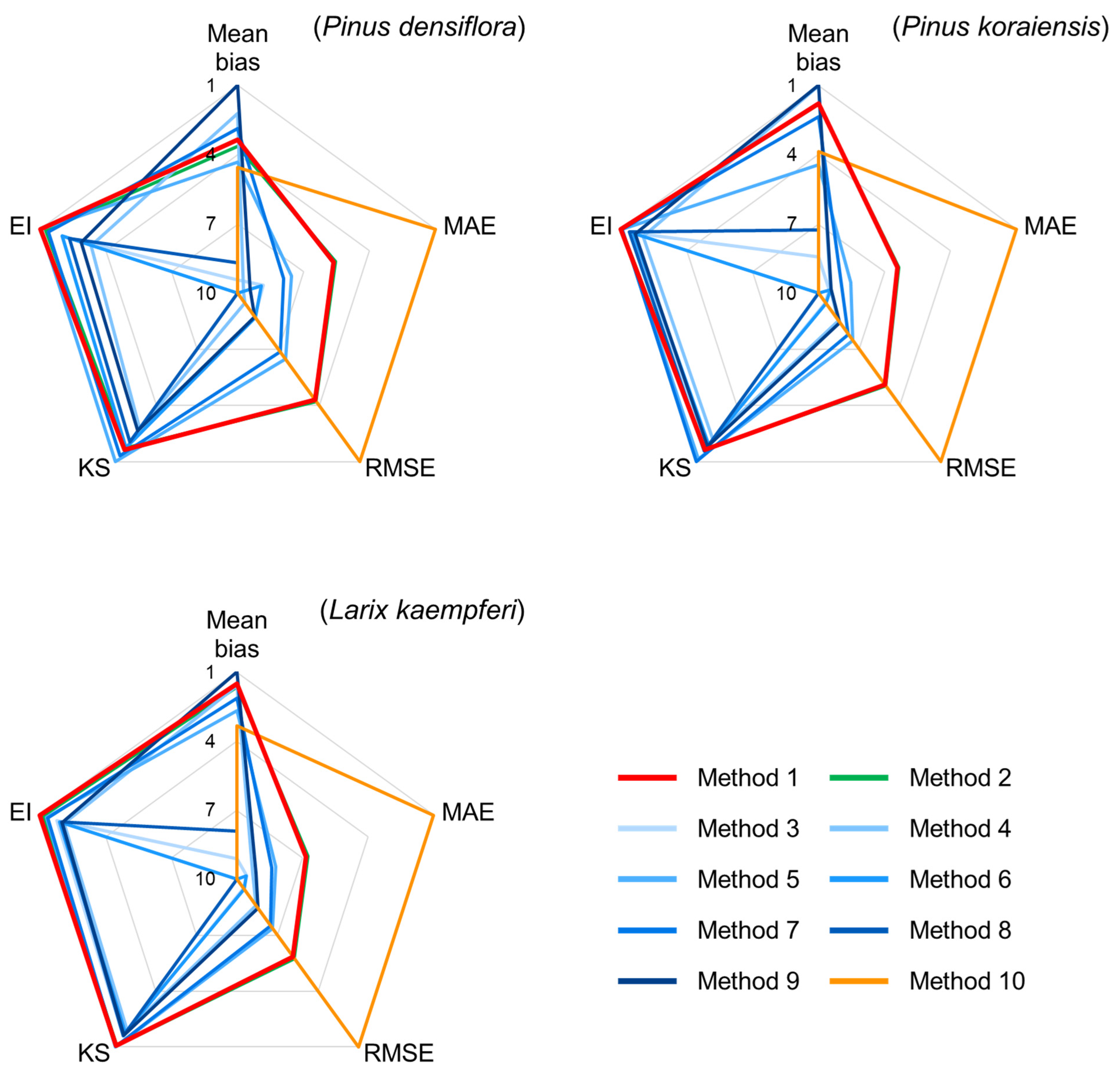
Relative ranks of statistics calculated for each parameter recovery method were determined (Figure 2). Relative ranks were determined based on the principle that lower values of goodness-of-fit statistics indicate greater performance of a parameter recovery method; therefore, the highest rank indicates the best performance, while the lowest rank indicates the poorest. For all three species, the method with the best and worst results for each statistic was consistent. Method 10 ranked highest for the MAE and the RMSE but lowest for the KS statistic and the EI. Method 8 had the lowest rank for both MAE and RMSE, while Method 6 ranked lowest for the mean bias. Method 9 was the highest rank for the mean bias, and Method 5 ranked highest for KSq. Method 1 ranked highest for the EI.
The moment-based parameter recovery methods, which are Methods 1 and 2, generally showed superior rankings, except for the EI, where Method 1 ranked best. In contrast, the percentile-based parameter recovery methods, which are Methods 3–9, and the hybrid method, which is Method 10, showed inconsistent rankings for each statistic. The hybrid method, in particular, performed well in such statistics as the mean bias, the MAE, and the RMSE, but ranked lowest for goodness-of-fit statistics such as the KS statistic and the EI.
In overall ranks, the moment-based parameter recovery methods, Methods 1 and 2, achieved high ranks, with values of 1.00 and 1.24 for Korean red pine, 1.00 and 1.01 for Korean white pine, and 1.00 and 1.05 for Japanese larch, respectively. The lowest-ranking methods by species were Method 8 for Korean red pine and Method 6 for both Korean white pine and Japanese larch. Although Method 7 was selected as the best parameter recovery method for Korean red pine, Korean white pine, and Japanese larch in [28], it ranked relatively low, with values of 3.32 for Korean red pine, 3.86 for Korean white pine, and 3.27 for Japanese larch in this study. Meanwhile, Method 1, which ranked highest in this study, was also reported as the optimal parameter recovery method by Poudel [36] and Poudel and Cao [10]. Therefore, the best diameter distribution model was selected as the Weibull function using the moment-based parameter recovery method, specifically Method 1.
A radar chart was used to visualize the relative ranks of the goodness-of-fit statistics (Figure 2). The radar chart allows an overall assessment of the performance of each parameter recovery method based on the area covered. The widest area was observed for Method 1, which is similar to Method 2, but with a slight difference. Method 10 was skewed toward the right in terms of the RMSE and the MAE, while the areas formed by the remaining methods were almost indistinguishable from one another.
The goodness-of-fit index results for Method 1, selected as the best parameter recovery method, are shown in Table 4. The average EIs were 339 for Korean red pine, 279 for Korean white pine, and 286 for Japanese larch. The average KSq values were 0.55 for Korean red pine, 0.51 for Korean white pine, and 0.50 for Japanese larch, showing little difference between the species. The number of cases rejected at α = 0.1 was 24 cases (5.8%) for Korean red pine, 12 cases (2.1%) for Korean white pine, and 7 cases (1.3%) for Japanese larch.

3.2. Models for Parameter Recovery

To predict the recovered Weibull parameters using the estimated parameter recovery method, models were developed for the mean DBH, the DBH variance, and the minimum DBH (Table 5). Compared to the mean DBH and DBH variance models, the minimum DBH model had a p-value exceeding 0.01 for H d , resulting in its removal from the independent variables. For the mean DBH model, the R2 for Korean red pine was 0.9728, with 1 / A g e , the reciprocal of age, having the highest effect on the mean DBH. For Korean white pine, the R2 was 0.9747, with l n A g e , which is the natural logarithm of age, as the variable with the highest effect. For Japanese larch, the R2 was 0.9572, with l n H d , which is the natural logarithm of the dominant height, having the highest effect on the mean DBH.
For the DBH variance model, the R2 for Korean red pine was 0.8822, with l n A g e as the variable having the highest effect on the DBH variance. The R2 for Korean white pine was 0.7635, with l n A g e having the highest effect on the DBH variance. For Japanese larch, the R2 was 0.7585, with l n H d as the variable affecting the DBH variance. In the minimum DBH model, the R2 for Korean red pine was 0.8469, with 1 / A g e having the largest effect on the minimum DBH. For Korean white pine, the R2 was 0.7186, with 1 / A g e also being the variable with the highest effect. For Japanese larch, the R2 was 0.7190, with l n N , which is the natural logarithm of the number of stems, having the greatest effect on the minimum DBH.
In most models related to the characteristics of diameter distribution, age was the variable with the highest effect. Additionally, unlike the DBH variance, both mean DBH and minimum DBH were negatively affected by the number of stems as an independent variable. This is likely because as the number of stems decreases, the likelihood of dominant trees remaining increases. The residual plots of the final selected model were unbiased for the fitted values in all three species, with the residuals appearing randomly dispersed and showing no biased patterns with respect to each independent variable (Figures S1–S3).

3.3. Models for Parameter Prediction

To predict the Weibull parameters using the parameter prediction method, models were developed for parameters a, b, and c (Table 6). Compared to the parameter a and b models, the parameter c model had a p-value exceeding 0.01 for H d , resulting in its removal from the independent variables. For the model of parameter a, which determines the initial location of the Weibull distribution, the R2 for Korean red pine was 0.8586, with 1 / A g e , the reciprocal of age, having the highest effect on parameter a. For Korean white pine, the R2 was 0.7194, also with 1 / A g e as the variable with the highest effect on parameter a. For Japanese larch, the R2 was 0.7256, with l n N , the natural logarithm of the number of stems, having the highest effect on parameter a.
For the model of parameter b, which represents the scale of the Weibull distribution, the R2 for Korean red pine was 0.9374, with 1 / A g e as the variable with the highest effect on parameter b. For Korean white pine, the R2 was 0.9231, with 1 / A g e , again, as the variable with the highest effect on parameter b. For Japanese larch, the R2 was 0.8893, with l n H d , the natural logarithm of the dominant height, having the highest effect on parameter b.
For the model of parameter c, which represents the shape of the Weibull distribution, the R2 for Korean red pine was 0.7805, with l n N as the variable with the highest effect on parameter c. For Korean white pine, the R2 was 0.7032, with 1 / A g e as the most significant variable affecting parameter c. For Japanese larch, the R2 was 0.7437, with 1 / A g e also being the variable with the highest effect on parameter c.
The residual plots of the final selected parameter prediction model were unbiased for the fitted values in all the three species, with the residuals appearing randomly dispersed and showing no biased patterns with respect to each independent variable (Figures S4–S6).

3.4. Comparison Estimated Parameters

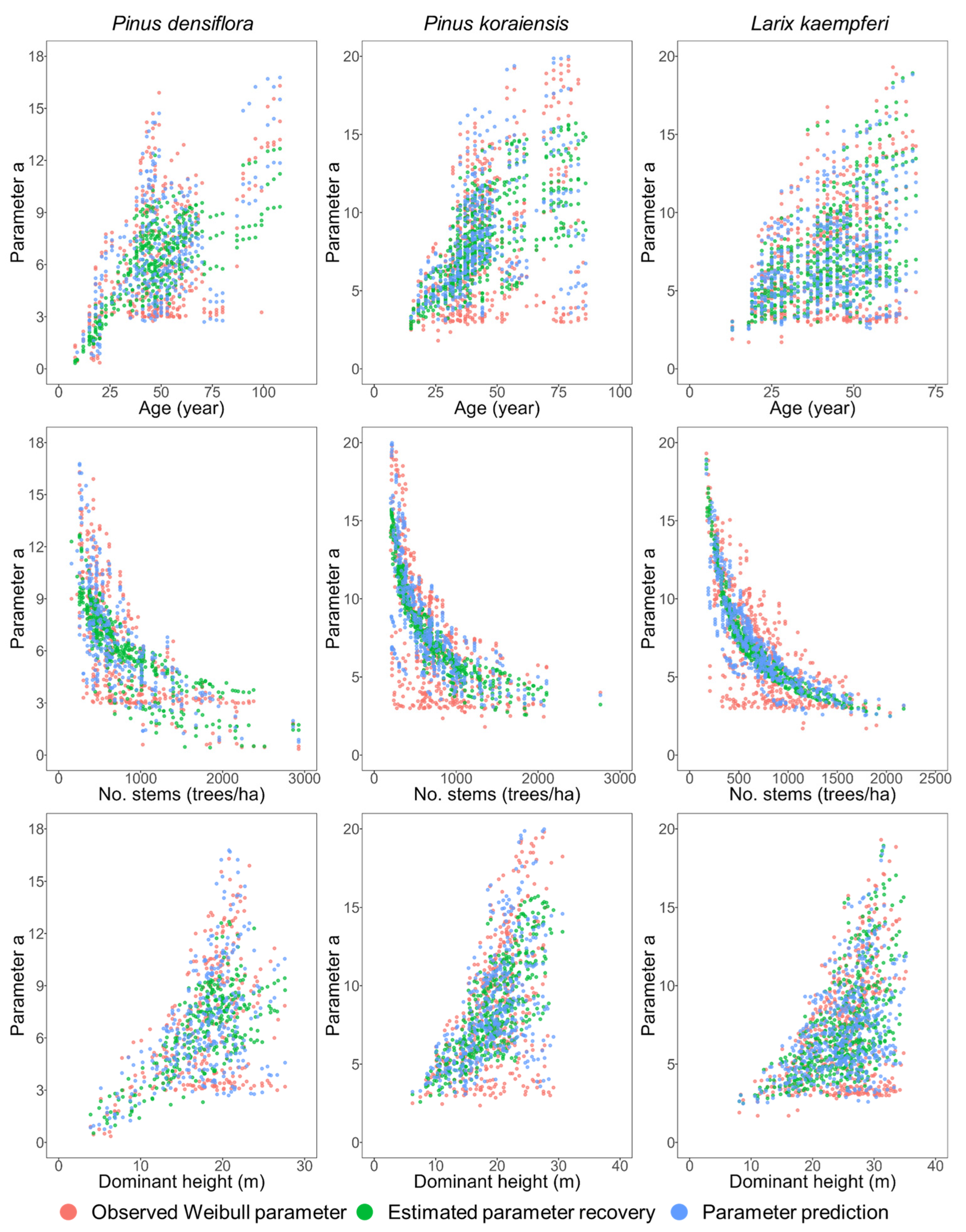
The parameters from three methods (recovered from the observed data, estimated using parameter recovery, and estimated using parameter prediction) were compared (Figure 3). The three types of parameters were evenly dispersed, and the two estimated parameters exhibited trends similar to the observed Weibull parameters. A similar trend in parameter a, which is determined by the initial location of the Weibull distribution function, was observed in all the three species. As age increased, the range of parameter a tended to spread. Generally, as age increases, the minimum DBH is likely to increase because the minimum DBH in the stand becomes relatively larger as trees grow. However, with high stand density and intense competition, diameter growth can be inhibited [43,44].
As the number of stems increased, parameter a was observed to decrease. As reported by Lee and Choi [45], the overall DBH is likely to be smaller in high-density stands. Conversely, as the number of stems decreases, stand density decreases as well, allowing more space for individual trees to grow, resulting in a higher overall DBH in the stand. An increase in the dominant height generally corresponded with an increase in the range of parameter a. Dominant height, which represents site productivity, is crucial for calculating the site index [46]. However, it is evident that an increase in the dominant height does not necessarily promote the minimum diameter growth.
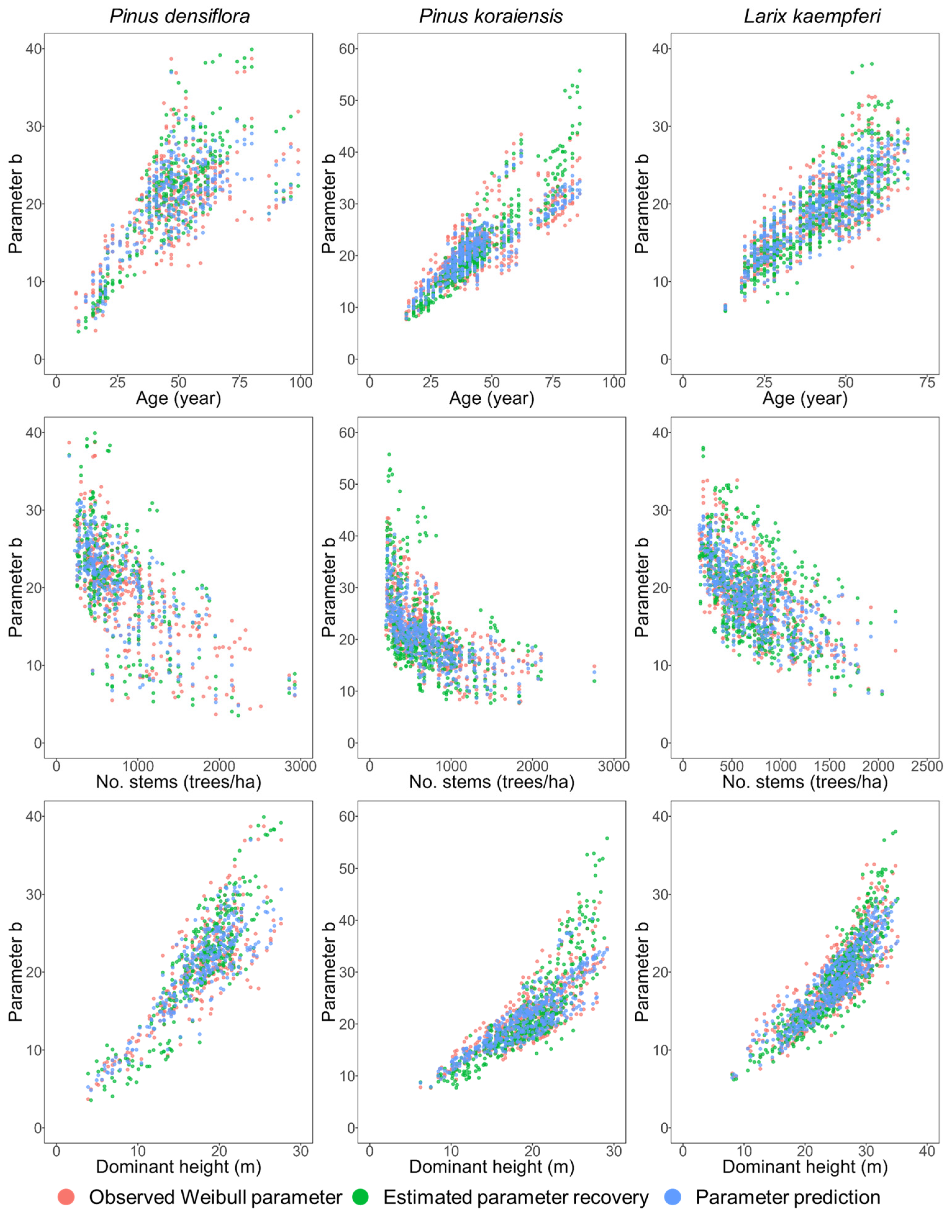
For parameter b, the three types of parameters were also evenly dispersed, and the two estimated parameters showed a tendency similar to the observed Weibull parameters (Figure 4). A similar tendency was shown in parameter b, which is represented by the scale of the Weibull distribution, by species. As age increased, parameter b tended to increase. When parameter b is smaller, the distribution skews to the left, indicating a higher proportion of smaller trees, while a larger value shifts the distribution to the right, indicating a higher proportion of large-diameter trees [47]. The trend of a higher proportion of large-diameter trees with increasing age is reasonable.
Unlike age, as the number of stems increased, parameter b showed a decreasing tendency. In high-density stands, the overall DBH in the stand tended to be smaller [45]. Conversely, in stands with large growing space, the DBH growth is greater. Therefore, the negative relationship between the number of stems and parameter b is reasonable. As the dominant height increased, parameter b also tended to increase. While parameter a exhibited a tendency to spread over a wider range, parameter b showed an increase within a consistent range. Dominant height, representing site productivity, may not be related to the diameter growth of the smallest trees within a stand, but it can be associated with the overall diameter distribution.
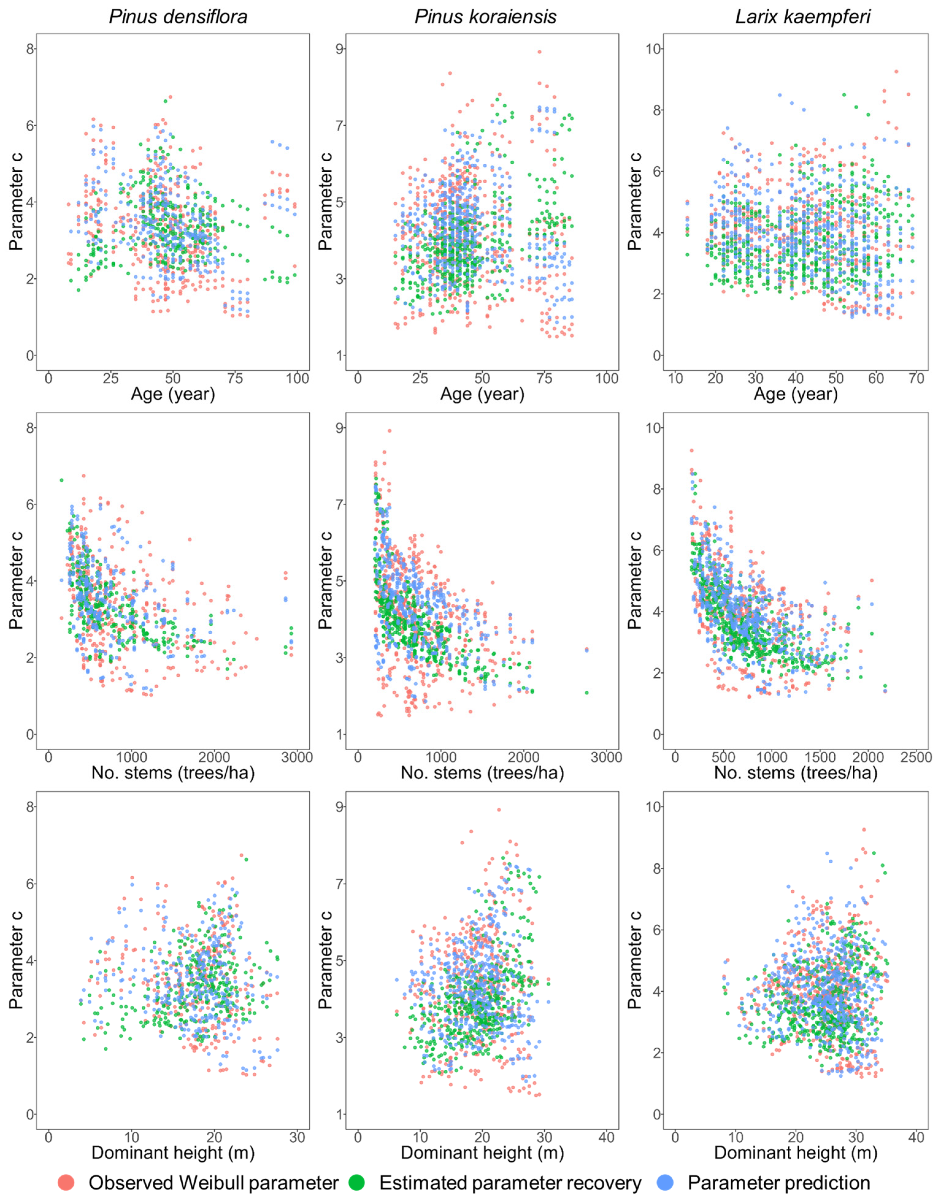
For parameter c, the three types of parameters were also evenly dispersed, and the two estimated parameters showed trends similar to the observed Weibull parameters (Figure 5). A similar tendency was shown in parameter c, which represents the shape of the Weibull distribution, by species. Unlike parameters a and b, parameter c showed no specific trend with age and dominant height. However, as the number of stems increased, parameter c tended to decrease. When parameter c is higher, diameter distribution becomes concentrated around a specific class. When stand density is high, differences in crown class cause variations in diameter growth over time, leading to a wider diameter distribution. In this regard, it is reasonable that, as the number of stems decreases, the distribution becomes more concentrated around a specific class, while a higher number of stems results in a wider diameter distribution.
To compare the estimated parameter recovery and parameter prediction, bias was calculated by subtracting the observed Weibull parameter from the predicted value (Figure 6). The bias indicated that parameter prediction performed better than estimated parameter recovery. When comparing parameter a, the Mean bias in parameter prediction ranged from 0.01 to 0.04, while in estimated parameter recovery, it ranged from −0.03 to −0.15. For parameter b, the Mean bias in parameter prediction was −0.07 to −0.10, while in the estimated parameter recovery, it ranged from 0.21 to 0.64. For parameter c, the Mean bias in parameter prediction ranged from −0.01 to 0.00, while in parameter recovery, it ranged from −0.17 to −0.36.
To determine whether the values estimated by each method differed from the observed Weibull parameters, a paired t-test was conducted (Table 7). In the estimated parameter recovery method, significant differences were observed for parameters b and c in Korean red pine, parameter c in Korean white pine, and parameter c in Japanese larch (p < 0.01, p < 0.05). In contrast, no significant differences were observed for any parameters in the parameter prediction method. Additionally, the p-values in the parameter prediction method were consistently higher than those in the estimated parameter recovery method.
Bias analysis and paired t-tests were conducted to compare the estimated parameter recovery and parameter prediction methods, and the results indicated that parameter prediction performed better than the estimated parameter recovery. Therefore, to predict diameter distribution using the Weibull function, the parameter prediction method in Table 6 provides higher accuracy when estimating the Weibull parameters. The parameter prediction model developed in this study is expected to serve as an applicational index for predicting yield.
The diameter distribution predicted using the Weibull parameters predicted by the two methods—the estimated parameter recovery and parameter prediction—was visualized against the observed data (Figure 7). The Weibull distribution from the estimated parameter recovery method was similar to the observed diameter distribution, though there were some cases with notable differences. Additionally, when compared to the distribution from the parameter prediction method, which closely represented the observed distribution, the estimated parameter recovery method showed relatively larger differences. As shown in Figure 7, the parameter prediction method also exhibited some cases of high bias. However, compared to the estimated parameter recovery method, the parameter prediction method had fewer cases with high bias.

4. Conclusions

This study was conducted to predict the number of stems by diameter class in Korean red pine, Korean white pine, and Japanese larch plantations using the Weibull function. The best diameter distribution model for each species was developed using 10 parameter recovery methods. Goodness-of-fit statistics were calculated for each method, and models were evaluated based on their relative rankings in the parameter recovery method. As a result, Method 1, which uses D 0 , D ¯ , and D v a r , was evaluated as the best diameter distribution model. To predict the recovered Weibull parameters, models were developed for D 0 , D ¯ , and D v a r . The models had high explanatory power, with R2 values ranging from 0.9572 to 0.9747 for D ¯ , from 0.7585 to 0.8822 for D v a r , and from 0.7186 to 0.8469 for D 0 . Models were also developed for each Weibull parameter to estimate the recovered Weibull parameters. Parameter a models had R2 values from 0.7194 to 0.8586, parameter b models ranged from 0.8893 to 0.9374, and parameter c models ranged from 0.7032 to 0.7805, all indicating high explanatory power. Additionally, the models developed in this study showed no bias, and the residuals were randomly dispersed.
To compare the estimated parameter recovery method and the parameter prediction method, bias analysis and paired t-tests were conducted. Parameter prediction had a lower bias than the estimated parameter recovery. Moreover, while the paired t-test showed significant differences (p < 0.001) for the estimated parameter recovery method, no significant differences were found for the parameter prediction method. The diameter distribution model developed in this study will enable efficient silvicultural practices and timber harvesting in forest management. By predicting the number of stems by diameter class, it will be possible to estimate the amount of large-diameter timber that can be produced within a stand. Additionally, applying a height growth model to estimate tree volume and calculating timber yield can provide fundamental information for establishing silvicultural systems and forest policies. Future studies should extend beyond the Weibull function to compare and evaluate various alternative models, further improving the accuracy and applicability of diameter distribution models.

Supplementary Materials

The following supporting information can be downloaded at: https://www.mdpi.com/article/10.3390/f16060961/s1, Figure S1. Residual plots for the mean DBH model by species. One of the models for the parameter recovery method. Figure S2. Residual plots for the DBH variance model by species. One of the models for the parameter recovery method. Figure S3. Residual plots for the minimum DBH model by species. One of the models for the parameter recovery method. Figure S4. Residual plots for the parameter a model by species. One of the models for the parameter prediction method. Figure S5. Residual plots for the parameter b model by species. One of the models for the parameter prediction method. Figure S6. Residual plots for the parameter c model by species. One of the models for the parameter prediction method.

Author Contributions

Conceptualization, S.J., D.L. and J.C.; methodology, S.J. and D.L.; investigation, S.J. and D.L.; data curation, S.J. and D.L.; formal analysis, S.J. and D.L.; software, S.J. and D.L.; resources, S.J., D.L. and J.C.; Validation, S.J., D.L. and J.C.; Visualization, S.J. and D.L; writing—original draft preparation, S.J.; writing—review and editing, S.J., D.L. and J.C.; supervision, J.C.; funding acquisition, J.C.; project administration, J.C. All authors have read and agreed to the published version of the manuscript.

Funding

This study was carried out with the support of the Basic Science Research Program through the National Research Foundation of Korea (NRF) funded by the Korean Ministry of Education (Grant No. NRF-2016R1D1A1B02011648).

Data Availability Statement

Data are contained within the article.

Acknowledgments

Financial support for data collection was provided by the National Forest Management Division of the Korea Forest Service. The Forest Resource Monitoring Center on Climate Change (FRMCCC) at the Kangwon National University provided data maintenance support.

Conflicts of Interest

The authors declare no conflict of interest. The funders had no role in the design of the study; in the collection, analyses, or interpretation of data; in the writing of the manuscript; or in the decision to publish the results.

References

  1. Burkhart, H.E.; Avery, T.E.; Bullock, B.P. Forest Measurements, 6th ed.; Waveland Press: Long Grove, IL, USA, 2019; ISBN 1-4786-3809-5. [Google Scholar]
  2. Guo, H.; Lei, X.; You, L.; Zeng, W.; Lang, P.; Lei, Y. Climate-Sensitive Diameter Distribution Models of Larch Plantations in North and Northeast China. For. Ecol. Manag. 2022, 506, 119947. [Google Scholar] [CrossRef]
  3. Russell, M.B.; Burkhart, H.E.; Amateis, R.L.; Prisley, S.P. Regional Locale and Its Influence on the Prediction of Loblolly Pine Diameter Distributions. South. J. Appl. For. 2012, 36, 198–203. [Google Scholar] [CrossRef]
  4. Lin, H.-T.; Lam, T.Y.; Peng, P.-H.; Chiu, C.-M. Embedding Boosted Regression Trees Approach to Variable Selection and Cross-Validation in Parametric Regression to Predict Diameter Distribution After Thinning. For. Ecol. Manag. 2021, 499, 119631. [Google Scholar] [CrossRef]
  5. Korea Forest Service. The 6th National Forest Plan (2018~2037); Korea Forest Service: Daejeon, Republic of Korea, 2018; p. 151.
  6. Korea Forest Service. Plant 30.9 Billion Trees by 2050 to Reduce Carbon Emissions by 34 Million Tons; Korea Forest Service: Daejeon, Republic of Korea, 2021; p. 7.
  7. Siipilehto, J.; Mehtätalo, L. Parameter Recovery vs. Parameter Prediction for the Weibull Distribution Validated for Scots Pine Stands in Finland. Silva Fenn. 2013, 47, 1057. [Google Scholar] [CrossRef]
  8. Maltamo, M.; Puumalainen, J.; Päivinen, R. Comparison of Beta and Weibull Functions for Modelling Basal Area Diameter Distribution in Stands of Pinus sylvestris and Picea abies. Scand. J. For. Res. 1995, 10, 284–295. [Google Scholar] [CrossRef]
  9. Cao, Q.V. Predicting Parameters of a Weibull Function for Modeling Diameter Distribution. For. Sci. 2004, 50, 682–685. [Google Scholar] [CrossRef]
  10. Poudel, K.P.; Cao, Q.V. Evaluation of Methods to Predict Weibull Parameters for Characterizing Diameter Distributions. For. Sci. 2013, 59, 243–252. [Google Scholar] [CrossRef]
  11. Liu, Y.-H.; Yen, T.-M. Combining Stand Diameter Distribution Quantified by the Weibull Function to Develop a Carbon Yield Model for Makino Bamboo (Phyllostachys makinoi Hayata). Forests 2025, 16, 436. [Google Scholar] [CrossRef]
  12. Siipilehto, J. Methods and Applications for Improving Parameter Prediction Models for Stand Structures in Finland. Diss. For. 2011, 124, 56. [Google Scholar] [CrossRef]
  13. Korea Forest Service. 2023 Statistical Yearbook of Forestry; Korea Forest Service: Daejeon, Republic of Korea, 2023.
  14. Korea Forest Research Institute. Commercial Tree Species 4 Larix Kampferi; Korea Forest Research Institute: Seoul, Republic of Korea, 2012; p. 180. [Google Scholar]
  15. Korea Forest Research Institute. Commercial Tree Species 3 Pinus Koraiensis; Korea Forest Research Institute: Seoul, Rebublic Korea, 2012; p. 168. [Google Scholar]
  16. Korea Forest Research Institute. Commercial Tree Species 1 Pinus Densiflora; Korea Forest Research Institute: Seoul, Rebublic Korea, 2012; p. 250. [Google Scholar]
  17. Lee, D.S. Studies on Growth Models for Larix Kaempferi, Pinus Koraiensis, and Pinus Densiflora in Korea; Kangwon National University: Chuncheon, Republic of Korea, 2015. [Google Scholar]
  18. Jin, H.J. A Study on Model Development of Stand Growth and Adequate Thinning Criteria for Major Coniferous Species Using Stand Density Index; Kangwon National University: Chuncheon, Republic of Korea, 2024. [Google Scholar]
  19. Lee, D.S.; Choi, J. A study on stand structure and growth characteristics of Korean White Pine (Pinus koraiensis) in North Central Region of Gangwon Province. J. For. Environ. Sci. 2014, 30, 101–106. [Google Scholar] [CrossRef]
  20. Weibull, W. A Statistical Distribution Function of Wide Applicability. J. Appl. Mech. 1939, 18, 293–297. [Google Scholar] [CrossRef]
  21. Son, Y.M.; Pyo, J.K.; Kim, S.W.; Lee, K.H. Prediction of stand volume and carbon stock for Quercus variabilis using Weibull distribution model. J. Korean Soc. For. Sci. 2012, 101, 599–605. [Google Scholar]
  22. Yun, J.W. Studies on the Application of Weibull Distribution in Forestry (I)–Estimation of Diameter Distribution. J. Korean For. Soc. 1983, 59, 46–50. [Google Scholar]
  23. Lee, S.J. A Study on the Management of Pinus densiflora Forests by Spatial Scale to Prevent the Spread of Crown Fires; Kongju National University: Gongju, Republic of Korea, 2022. [Google Scholar]
  24. Lee, Y.J.; Coble, D.W. New Diameter Distribution Model for Unmanaged Loblolly Pine Plantations in East Texas. South. J. Appl. For. 2006, 30, 13–20. [Google Scholar] [CrossRef]
  25. Cao, Q.V.; Burkhart, H.E.; Lemin, R.C. Diameter Distributions and Yields of Thinned Loblolly Pine Plantations; Virginia Tech: Blacksburg, VA, USA, 1982. [Google Scholar]
  26. Hyink, D.M.; Moser, J.W. A Generalized Framework for Projecting Forest Yield and Stand Structure Using Diameter Distributions. For. Sci. 1983, 29, 85–95. [Google Scholar]
  27. Lynch, T.B.; Moser, J.W. A Growth Model for Mixed Species Stands. For. Sci. 1986, 32, 697–706. [Google Scholar] [CrossRef]
  28. Lee, D.S. Integrated Growth and Yield Models of Pinus densiflora, Pinus koraiensis, and Larix kaempferi Stands in Korea. Ph.D. Thesis, Kangwon National University, Chuncheon, Republic of Korea, 2018. [Google Scholar]
  29. Knowe, S.A.; Radosevich, S.R.; Shula, R.G. Basal Area and Diameter Distribution Prediction Equations for Young Douglas-Fir Plantations with Hardwood Competition: Coast Ranges. West. J. Appl. For. 2005, 20, 77–93. [Google Scholar] [CrossRef]
  30. McTague, J.P.; Bailey, R.L. Compatible Basal Area and Diameter Distribution Models for Thinned Loblolly Pine Plantations in Santa Catarina, Brazil. For. Sci. 1987, 33, 43–51. [Google Scholar] [CrossRef]
  31. Bailey, R.L.; Burgan, T.M.; Jokela, E.J. Fertilized Midrotation-Aged Slash Pine Plantations—Stand Structure and Yield Prediction Models. South. J. Appl. For. 1989, 13, 76–80. [Google Scholar] [CrossRef]
  32. Brooks, J.R.; Borders, B.E.; Bailey, R.L. Predicting Diameter Distributions for Site-Prepared Loblolly and Slash Pine Plantations. South. J. Appl. For. 1992, 16, 130–133. [Google Scholar] [CrossRef]
  33. Coble, D.W.; Lee, Y.J. A New Diameter Distribution Model for Unmanaged Slash Pine Plantations in East Texas. South. J. Appl. For. 2008, 32, 89–94. [Google Scholar] [CrossRef]
  34. Jiang, L.; Brooks, J.R. Predicting Diameter Distributions for Young Longleaf Pine Plantations in Southwest Georgia. South. J. Appl. For. 2009, 33, 25–28. [Google Scholar] [CrossRef]
  35. Lee, S.J.; Kim, S.Y.; Lee, B.D.; Lee, Y.J. Estimation of canopy fuel characteristics for Pinus densiflora stands using diameter distribution models: Forest managed stands and unmanaged stands. J. Korean Soc. For. Sci. 2018, 107, 412–421. [Google Scholar] [CrossRef]
  36. Poudel, K.P. Evaluation of Methods to Predict Weibull Parameters for Characterizing Diameter Distributions; Louisiana State University and Agricultural and Mechanical College: Baton Rouge, LA, USA, 2011. [Google Scholar]
  37. Siipilehto, J. Local Prediction of Stand Structure Using Linear Prediction Theory in Scots Pine-Dominated Stands in Finland. Silva Fenn. 2011, 45, 669–692. [Google Scholar] [CrossRef]
  38. Eid, T. Models for Prediction of Basal Area Mean Diameter and Number of Trees for Forest Stands in South-Eastern Norway. Scand. J. For. Res. 2001, 16, 467–479. [Google Scholar] [CrossRef]
  39. Lee, D.; Siipilehto, J.; Beuker, E.; Fahlvik, N.; Liziniewicz, M.; Hynynen, J. Multivariate Mixed-Effects Models for Stand Characteristics of Hybrid Aspen Plantations in Southern Finland and Southern Sweden. For. Ecol. Manag. 2023, 541, 121066. [Google Scholar] [CrossRef]
  40. Xie, L.; Wang, T.; Miao, Z.; Hao, Y.; Dong, L.; Li, F. Considering Random Effects and Sampling Strategies Improves Individual Compatible Biomass Models for Mixed Plantations of Larix olgensis and Fraxinus mandshurica in Northeastern China. For. Ecol. Manag. 2023, 537, 120934. [Google Scholar] [CrossRef]
  41. Bronisz, K.; Mehtätalo, L. Seemingly Unrelated Mixed-Effects Biomass Models for Young Silver Birch Stands on Post-Agricultural Lands. Forests 2020, 11, 381. [Google Scholar] [CrossRef]
  42. Ciceu, A.; Garcia-Duro, J.; Seceleanu, I.; Badea, O. A Generalized Nonlinear Mixed-Effects Height–Diameter Model for Norway Spruce in Mixed-Uneven Aged Stands. For. Ecol. Manag. 2020, 477, 118507. [Google Scholar] [CrossRef]
  43. Lee, D.K.; Kwon, K.W.; Kim, J.H.; Kim, G.T. Silviculture; Hyangmunsa: Seoul, Republic of Korea, 2010. [Google Scholar]
  44. Lee, D.S.; Jung, S.H.; Choi, J.K. Analysis of tree growth characteristics by first and second thinning in Korean White Pine plantations. J. Korean Soc. For. Sci. 2022, 111, 150–164. [Google Scholar] [CrossRef]
  45. Lee, D.S.; Choi, J.K. Evaluating Maximum Stand Density and Size–Density Relationships Based on the Competition Density Rule in Korean Pines and Japanese Larch. For. Ecol. Manag. 2019, 446, 204–213. [Google Scholar] [CrossRef]
  46. Lee, D.S.; Beuker, E.; Viherä-Aarnio, A.; Hynynen, J. Site Index Models with Density Effect for Hybrid Aspen (Populus tremula L. × P. tremuloides Michx.) Plantations in Southern Finland. For. Ecol. Manag. 2021, 480, 118669. [Google Scholar] [CrossRef]
  47. Yun, J.W.; Cho, H.K. Estimating Diameter Distribution with the Weibull Distribution–Case of Korea Black Pine (Pinus thunbergii) Stands on the Eastern Sea Coast of Korea. J. Korean Soc. For. Sci. 1991, 80, 420–426. [Google Scholar]
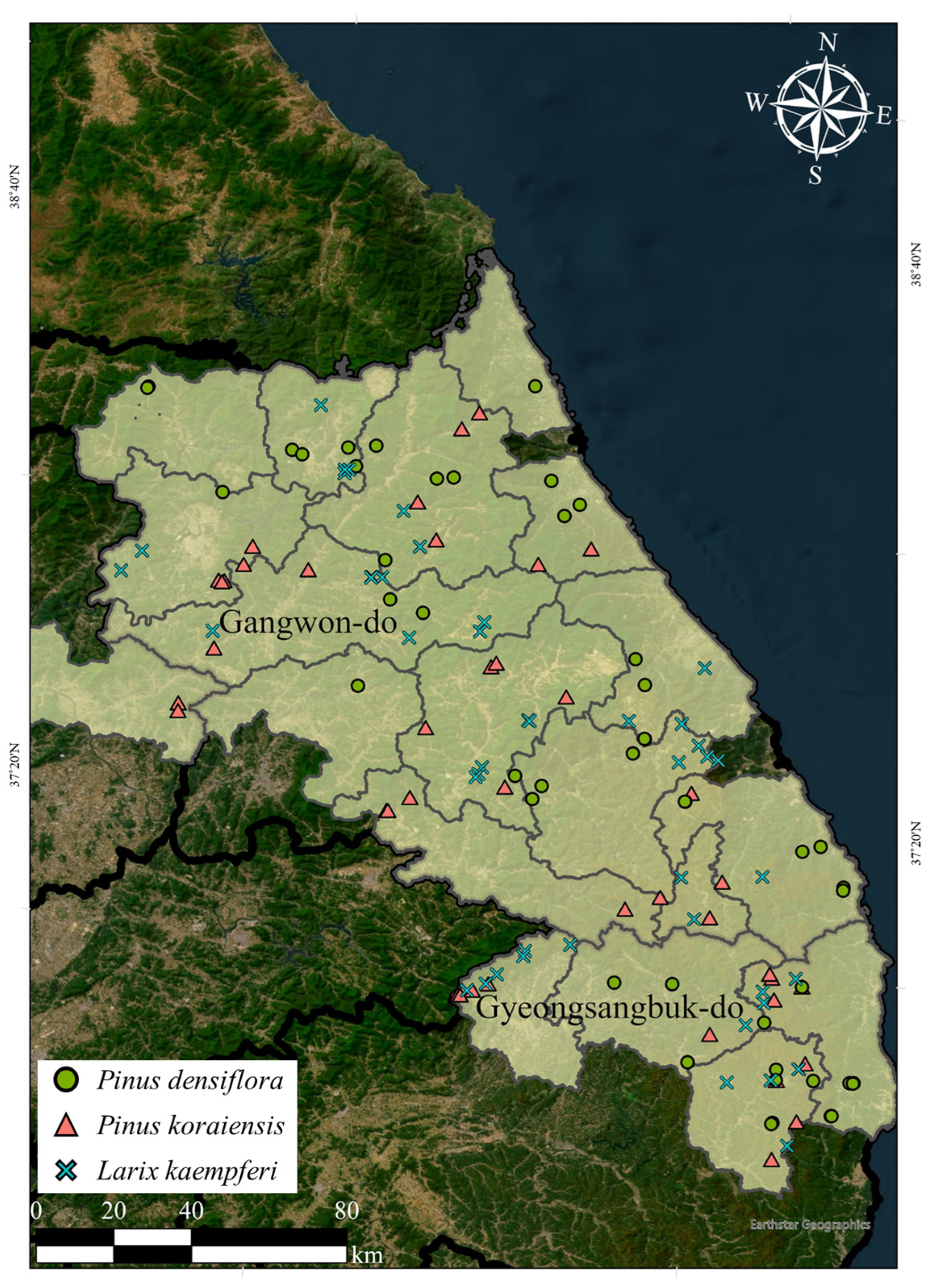
Figure 1. Map of the experimental sites for the three coniferous species in Gangwon and North Gyeongsang Provinces of South Korea. Each experimental site consists of three plots.
Forests 16 00961 g001
Figure 2. Radar chart of relative ranks of parameter recovery methods by the goodness-of-fit statistics. The red line represents Method 1, which was selected as the optimal parameter recovery method. The green line represents Method 2, which is a moment-based method. The blue line represents percentile-based methods (Methods 3–9), and the orange line represents Method 10, which is a hybrid method. The mathematical equations for these parameter recovery methods are detailed in Table 2.
Forests 16 00961 g002
Figure 3. Scatter plots for parameter a and independent variables of the observed parameter recovery method, the estimated parameter recovery method, and the parameter prediction method by species.
Forests 16 00961 g003
Figure 4. Scatter plots for parameter b and independent variables of the observed parameter recovery method, the estimated parameter recovery method, and the parameter prediction method by species.
Forests 16 00961 g004
Figure 5. Scatter plots for parameter c and independent variables of the observed parameter recovery method, the estimated parameter recovery method, and the parameter prediction method by species.
Forests 16 00961 g005
Figure 6. Box-and-whisker plots of bias in the estimated parameter recovery and parameter prediction. Bias is calculated by subtracting the observed Weibull parameter from the estimated Weibull parameter in this study.
Forests 16 00961 g006
Figure 7. Examples of the observed diameter histograms and the diameter distribution using the Weibull function with the parameters estimated in this study in the stands of Pinus densiflora (Pd), P. koraiensis (Pk), and Larix kaempferi (Lk). The columns represent the species, and the rows represent different stages of stand development with stand age. Age classes are defined as young (under 20 years), mature (20–39 years), and old (40 years or older). Hd is the dominant height (m); N is the number of stems per hectare (trees per ha−1); and D is the mean diameter (cm).
Forests 16 00961 g007
Table 1. Summary statistics of the experimental sites for Pinus densiflora, Pinus koraiensis, and Larix kaempferi.
SpeciesStatisticsAge
(years)
DBH
(cm)
Height
(m)
No. of Stems
(trees per ha−1)
Pinus densiflora
(n = 49)
Mean4120.913.4913
SD2010.75.2571
Min83.20.9155
Max10882.030.13405
Pinus koraiensis
(n = 54)
Mean4024.316.1809
SD149.24.6443
Min153.61.7176
Max8665.032.32155
Larix kampferi
(n = 49)
Mean3822.820.4722
SD138.35.9374
Min193.43.2169
Max6963.636.72037
Note: n is the total number of the experimental sites. The data of individual trees were used for calculating the statistics, with the number of trees being 14,677 for Pinus densiflora, 17,484 for P. koraiensis, and 14,508 for Larix kaempferi.
Table 2. Equations for parameter recovery for the Weibull distribution.
MethodVariables to Recover the Weibull ParametersEquations
Moment-based1 D 0 , D ¯ , and D v a r a = 0.5 D 0
b = D ¯ a G 1
c is obtained from b 2 G 2 G 1 2 D v a r = 0
2 D 0 , D q , and D v a r a = 0.5 D 0
b = a G 1 / G 2 + [ a / G 2 2 G 1 2 G 2 + D q 2 / G 2 ] 0.5
c is obtained from b 2 G 2 G 1 2 D v a r = 0
Percentile-based3 D 0 , D 63 , and D 31 a = 0.5 D 0
b = D 63 a [ l n ( 1 0.63 ) ] 1 / c
c = l n ( l n ( 1 0.63 ) l n ( 1 0.31 ) ) ln D 63 a l n ( D 31 a )
4 D 0 , D 50 , and D 95 a = 0.5 D 0
b = D 50 a [ l n ( 1 0.50 ) ] 1 / c
c = l n ( l n ( 1 0.95 ) l n ( 1 0.50 ) ) ln D 95 a l n ( D 50 a )
5 D 0 , D 50 , D 95 , and D 25 a = 0.5 D 0
b = D 50 a [ l n ( 1 0.50 ) ] 1 / c
c = l n ( l n ( 1 0.95 ) l n ( 1 0.25 ) ) ln D 95 a l n ( D 25 a )
6 D 0 , D 50 , D 63 , and D 31 a = 0.5 D 0
b = D 50 a [ l n ( 1 0.50 ) ] 1 / c
c = l n ( l n ( 1 0.63 ) l n ( 1 0.31 ) ) ln D 63 a l n ( D 31 a )
7 D 0 , D q , D 95 , and D 25 a = 0.5 D 0
b = a G 1 / G 2 + [ a / G 2 2 G 1 2 G 2 + D q 2 / G 2 ] 0.5
c = l n ( l n ( 1 0.95 ) l n ( 1 0.25 ) ) ln D 95 a l n ( D 25 a )
8 D 0 , D q , D 63 , and D 31 a = 0.5 D 0
b = a G 1 / G 2 + [ a / G 2 2 G 1 2 G 2 + D q 2 / G 2 ] 0.5
c = l n ( l n ( 1 0.63 ) l n ( 1 0.31 ) ) ln D 63 a l n ( D 31 a )
9 D 0 , D 95 , and D ¯ a = 0.5 D 0
b = D 95 a [ l n ( 1 0.95 ) ] 1 / c
c is obtained from a + b Γ G 1 D ¯ = 0
Hybrid10 D 0 , D q , D 25 , D 50 , and D 95 a = ( n 1 / 3 D 0 D 50 ) / ( n 1 / 3 1 )
b = a G 1 / G 2 + [ a / G 2 2 G 1 2 G 2 + D q 2 / G 2 ] 0.5
c = l n ( l n ( 1 0.95 ) l n ( 1 0.25 ) ) ln D 95 a l n ( D 25 a )
Note: a, b, and c are the Weibull parameters; D 0 is the minimum DBH in each stand (cm); D ¯ is the mean DBH in each stand (cm); G i is Γ ( 1 + i / c ) ; Γ is the complete gamma function; D v a r is the DBH variance in each stand (cm2); D q is the quadratic mean diameter in each stand (cm); ln() is the natural logarithm; D p is the diameter at breast height (DBH) corresponding to the pth percentile within a stand (cm); and n is the number of stems (trees per plot−1).
Table 3. Mean goodness-of-fit statistics of the Weibull diameter distribution model by parameter recovery methods.
SpeciesMethodMean BiasMAERMSEKSqEI
Pinus
densiflora
(n = 411)
166.377.797.70.55339.4
266.377.697.70.55341.9
366.478.598.50.55349.3
466.378.798.60.57362.6
566.378.298.10.54339.9
666.478.598.50.55349.3
766.378.398.20.54343.1
866.478.898.70.56352.7
966.278.798.50.57358.0
1066.376.597.10.70429.6
Pinus koraiensis
(n = 554)
157.668.484.00.51278.9
257.668.484.00.51279.5
357.769.585.10.51287.4
457.669.484.90.53297.9
557.669.184.60.49280.0
657.769.485.10.52289.6
757.669.384.70.49279.9
857.669.685.20.51286.2
957.669.484.80.51291.6
1057.666.682.90.78449.3
Larix kaempferi
(n = 537)
161.372.087.80.50286.0
261.372.087.70.50288.2
361.573.088.80.52299.8
461.372.988.60.53305.8
561.372.588.20.50291.2
661.573.188.80.52302.1
761.372.688.20.50292.3
861.573.289.00.52303.4
961.372.988.50.52303.8
1061.369.786.40.79446.4
Note: MAE is the mean absolute error; RMSE is the root mean square error; KSq is the Kolmogorov–Smirnov statistic quotient; EI is the error index; and n is the total number of plot level observations, determined by considering the number of sites, the number of plots per site, and the number of measurements.
Table 4. Goodness-of-fit statistics for Method 1 selected as the optimal parameter recovery method by species.
SpeciesError IndexKolmogorov–Smirnov
Statistic Quotient
Rejection Cases, Kolmogorov–Smirnov Statistic, 10% LevelThe Proportion of Rejected Cases (%)
Pinus densiflora
(n = 411)
339 ± 2260.55 ± 0.26245.8
(46–1606)(0.17–1.93)
Pinus koraiensis
(n = 554)
279 ± 1610.51 ± 0.19122.1
(49–1482)(0.17–1.62)
Larix kaempferi
(n = 537)
286 ± 1640.50 ± 0.1971.3
(50–1369)(0.15–1.78)
Note: n is the total number of plot level observations, determined by considering the number of sites, the number of plots per site, and the number of measurements. Statistics represent the means ± SD (min–max).
Table 5. Parameter estimates and fit statistics for the models to predict the mean DBH, the DBH variance, and the minimum DBH by species for the Weibull distribution.
Dependent
Variable
SpeciesFixed EffectsnRandom EffectResidualR2RMSEMAEMAPE
std(u) std ( ε )
D ¯ Pd l n D ¯ = 4.5149 13.6354 1 A g e + 0.0321 H d 0.2414 l n N 4110.12860.07160.97280.06590.05040.0167
Pk l n D ¯ = 2.2003 + 0.5742 l n A g e + 0.0139 H d 0.2091 l n N 5540.11800.05930.97470.05560.04220.0131
Lk l n D ¯ = 2.6123 + 0.0050 A g e + 0.5957 l n H d 0.2426 l n N 5370.08890.06390.95720.06100.04530.0144
D v a r Pd l n D v a r = 4.2756 + 1.2703 l n A g e + 0.0636 H d + 0.2844 l n N 4110.52440.33240.88220.30670.22960.0756
Pk l n D v a r = 5.3605 + 1.1971 l n A g e + 0.0542 H d + 0.4849 l n N 5540.52130.42150.76350.39700.28910.0931
Lk l n D v a r = 11.9627 + 0.7778 l n A g e + 2.1086 l n H d + 0.8648 l n N 5370.51290.41410.75850.39700.32320.1080
D 0 Pd l n D 0 = 5.9319 21.4202 1 A g e 0.4570 l n N 4110.36290.25560.84690.23650.17680.0908
Pk l n D 0 = 6.2840 12.9302 1 A g e 0.5081 l n N 5540.25390.27980.71860.26500.18440.0757
Lk l n D 0 = 6.7683 + 0.0056 A g e 0.6923 l n N 5370.21590.28960.71900.27780.21410.0909
Note: D ¯ is the mean DBH (cm); D v a r is the DBH variance (cm2); D 0 is the minimum DBH (cm); Pd is Pinus densiflora; Pk is P. koraiensis; Lk is Larix kaempferi; n is the total number of plot level observations, determined by considering the number of sites, the number of plots per site, and the number of measurements; std(u) is the standard deviation of the random effect at the experimental site level; std(ε) is the standard deviation of the residual in model performance; R2 is the coefficient of determination; RMSE is the root mean square error; MAE is the mean absolute error; MAPE is the mean absolute percentage error. All the parameters were significant (p < 0.05). The model includes a random effect for experimental site location.
Table 6. Parameter estimates and fit statistics for the models to predict the Weibull parameters by species for the Weibull distribution.
Dependent
Variable
SpeciesFixed EffectsnRandom EffectResidualR2RMSEMAEMAPE
std(u) std ( ε )
aPd l n a = 4.3011 15.0873 1 A g e + 0.0302 H d 0.4184 l n N 4110.36980.25120.85860.23190.17130.1235
Pk l n a = 5.3820 11.7177 1 A g e + 0.0536 l n H d 0.5047 l n N 5540.25470.28010.71940.26500.18440.1088
Lk l n a = 6.4309 + 0.0078 A g e 0.1275 l n H d 0.6994 l n N 5370.22470.28880.72560.27670.21320.1328
bPd l n b = 3.9111 12.4958 1 A g e + 0.0307 H d 0.1806 l n N 4110.11480.09830.93740.09110.06960.0243
Pk l n b = 3.0620 15.7361 1 A g e + 0.0227 H d 0.0001 l n N 5540.10560.08730.92310.08220.06330.0209
Lk l n b = 0.4781 + 0.0025 A g e + 0.7594 l n H d 0.0001 l n N 5370.09240.09010.88930.08610.06800.0234
cPd l n c = 3.7630 0.0050 A g e 0.3559 l n N 4110.26020.16930.78050.15660.12120.1967
Pk l n c = 3.5660 + 6.1108 1 A g e 0.3622 l n N 5540.24130.19520.70320.18410.13450.1213
Lk l n c = 4.5671 + 14.6297 1 A g e 0.5650 l n N 5370.20000.19640.74370.18780.15050.1487
Note: Pd is Pinus densiflora; Pk is P. koraiensis; Lk is Larix kaempferi; std(u) is the standard deviation of the random effect at the experimental site level; std(ε) is the standard deviation of the residual in model performance; R2 is the coefficient of determination; RMSE is the root mean square error; MAE is the mean absolute error; MAPE is the mean absolute percentage error; and n is the total number of plot level observations, determined by considering the number of sites, the number of plots per site, and the number of measurements. All the parameters were significant (p < 0.01).
Table 7. Statistics for the paired t-test of the estimated parameter recovery and parameter prediction. Paired t-test was conducted to compare the observed Weibull parameters with the estimated parameters.
MethodSpeciesParameterMeanSDD.F.t-ValuePr > |t|
Estimated
parameter recovery
Pda−0.2412.472311−1.720.086
b0.6433.4653.280.001
c−0.1711.382−2.180.030
Pka−0.1592.914449−1.160.247
b0.2454.2391.230.220
c−0.3581.615−4.71<0.001
Lka−0.0262.337535−0.260.794
b0.2142.8011.770.077
c−0.3111.369−5.25<0.001
Parameter predictionPda0.0401.3983110.500.615
b−0.0882.013−0.770.439
c−0.0090.530−0.310.758
Pka0.0191.9414490.210.837
b−0.0701.962−0.750.452
c−0.0030.695−0.100.919
Lka0.0121.9665350.140.892
b−0.1021.814−1.300.193
c−0.0060.770−0.190.850
Note: SD is the standard deviation; D.F. is the degree of freedom; Pd is Pinus densiflora; Pk is P. koraiensis; Lk is Larix kaempferi.
Disclaimer/Publisher’s Note: The statements, opinions and data contained in all publications are solely those of the individual author(s) and contributor(s) and not of MDPI and/or the editor(s). MDPI and/or the editor(s) disclaim responsibility for any injury to people or property resulting from any ideas, methods, instructions or products referred to in the content.