Agroforestry in the Soil and Water Conservation of Karst Can Improve Rural Eco-Revitalization: Evidence from the Core Area of the South China Karst

Abstract

Agroforestry (AF) effectively enhances ecological restoration and soil–water conservation (SWC), yet the relationship among soil and water conservation agroforestry (SWCAF) in karst soil, water loss (SWL) and rural eco-revitalization (RER) remains unclear, which may hinder the ecological restoration process around the world. This study aims to reveal whether SWCAF in karst areas improves RER through SWC benefits, ecosystem service (ES) enhancement and rural ecological environment quality (REEQ) improvement. We take Guizhou Province, the core area of the South China Karst (SCK), as the study area and 2010–2020 as the study period. By using the equivalent factor method, the remote sensing ecological index (RSEI) model, bivariate spatial autocorrelation and the panel vector autoregressive (PVAR) model, the study reveals SWCAF’s ecological benefits and its interaction mechanism with RER. Key findings reveal the following: (1) SWCAF reduced the area of SWL by 14.93% by converting cropland into forests. (2) The AF ecosystem service value (AFESV) increased by CNY 9.181 billion, and the forest-related AFESV increases represented 184% of the total AFESV, while REEQ showed an overall positive trend in the western SWC area. (3) The AFESV has an obvious synergistic effect with REEQ (r = 0.60) and obvious positive synergy with SWL (r = 0.69), and its spatial correlation increases over time. (4) The PVAR model verified that there is a bidirectional Granger causal relationship between the AFESV and RER, showing dynamic positive and negative alternating influences. This research study reveals that SWCAF drives RER through the dual path of SWL control and value-added ecological services, among which the forest ecosystem plays a core role. In the future, it is necessary to optimize the diversity of AF structures to avoid ecological service trade-offs. This research study provides a scientific basis for decision making and the ecological management of SWC in karst soils globally.

1. Introduction

Land degradation has become an urgent challenge threatening global ecosystem services and human well-being. Soil erosion (SWL), as the core driving factor of land degradation, causes a large amount of topsoil loss, directly leading to the loss of agricultural ecosystem functions and exacerbating global food security risks [1]. In fragile ecological areas, such as arid regions and karst landform areas, the vicious cycle of soil erosion further accelerates ecological collapse [2,3], highlighting the global strategic significance of soil and water conservation (SWC). For this reason, the international community has incorporated SWC into the framework of the Sustainable Development Goals (SDGs), and the United Nations Decade on Ecosystem Restoration (2021–2030) has explicitly proposed to reconstruct the human–land relationship with “nature-based solutions (NbSs)”, promoting the transformation of ecological restoration from being technology-dependent to being natural system-adaptive. Therefore, in-depth research on the role of NbSs in controlling SWL and restoring natural ecosystems is of great significance for soil and water conservation and livelihood security in ecologically fragile areas.

Agroforestry (AF), as a main NbS [4], combines perennial woody plants and components such as crops and animal husbandry, forming a multi-faceted, multi-level and multi-temporal ecosystem on the same land unit [5] and has become one of the important ecosystems worldwide. The term “AF” is used as a general term for various land-use systems, including agricultural land with scattered trees, family gardens with mixed trees and semi-natural forests with species composition adapted to human needs while retaining most of the structural features and ecological processes of natural forests [6]. It covers an area of approximately 1 billion hectares, accounting for 43% of the global agricultural land and involving more than 900 million people [7], mainly distributed in Asia, Africa, Europe, etc. [8]. Because it fills the gap among agriculture, forestry and animal husbandry and provides rich agroforestry ecosystem services (AFESs) and environmental benefits [9,10], it is regarded as one of the NbSs in ecological restoration. These benefits include raw material supply [11], soil health maintenance [12], biodiversity conservation [13], carbon sequestration [14] and so on. AF, with its excellent effect of soil and water conservation, is widely used in the ecological restoration of soil erosion [15]. The litter in the system forms a soil cover layer, which acts as a physical barrier to directly intercept erosion. Meanwhile, the canopy layer can also directly intercept rainwater, and perennial woody plants form a multi-level root network through the synergistic effect of deep roots and shallow-rooted crops, enhancing the shear strength and erosion resistance of soil [16]. AF can balance and improve services from the ecosystem. Research shows that it not only reduces the erosion modulus by 60%–70% compared with traditional farmland [17,18] but also increases cowpea yield by 162% and 81.9%, respectively [19].

In addition to controlling soil erosion, AF can also provide a variety of ecosystem services, such as material products, regulation services and cultural services. The assessment of its service value is of great reference significance for quantifying ecological benefits, promoting ecological protection and restoration, optimizing land use, balancing ecological and economic benefits, promoting the realization of ecological product value and assisting rural revitalization. The Value of the World’s Ecosystem Services and Natural Capital, published by Costanza et al. [20] in 1997, has triggered a global upsurge in research on the assessment of ecosystem service value (ESV). Subsequently, many scholars have conducted extensive research on the assessment of the agroforestry ecosystem service value (AFESV) based on the assessment framework and methods proposed by Costanza et al. and in combination with the actual situation. For example, in 2006, Olschewski et al. [21], in the study areas of Central Sulawesi, Indonesia and southern Manabi in Ecuador, evaluated the value of coffee pollination services in AF and non-forest areas, and it was found that agroforestry contributes to biodiversity conservation. German scholars Tsonkova et al. [22] developed an assessment tool for agroforestry ecosystem services based on empirical methods to evaluate the ecological regulation services and habitat supply support services of alleyway-planted agroforestry ecosystems. The results indicated that this planting system provided improvements in services such as erosion control and soil fertility compared with traditional agricultural systems. A scholar from Costa Rica, Latin America, integrated various indices of erosion control, carbon sequestration, nutrient cycling and biodiversity conservation and identified the trade-off–synergy among ecosystem services [23]. Leroux et al. [24] evaluated the spatial heterogeneity of each service supply in the Senegal Basin, Africa, by integrating field data of multiple ES indicators, the latest progress of remote sensing-derived information and different ES mapping methods. Most of these methods are based on a multi-index comprehensive evaluation system and have the characteristics of spatial heterogeneity analysis and system coupling analysis. By integrating remote sensing data, field observations and ecological models, they achieved the dynamic quantification and spatial visualization of service functions. The quantification of ecological service value (ESV) has always been regarded as an important tool for marginal decision making and policy making, and the ESV is one of the best indicators for studying environmental changes, providing an important reference for formulating reasonable ecological protection policies [25]. Ketema et al. [26] conducted an assessment of the agricultural ESV and found that agroforestry was the main contributor to the increase in the ESV in the densely populated areas of the Great Rift Valley in east Africa. Studying the economic value of agroforestry as a separate ecosystem can further improve the accuracy of ecosystem service valuation [27]. The ESV has been evaluated in the United Kingdom, France, Roman Transylvania and Germany in Europe; Sardinia, Greece, Portugal and Spain in the Mediterranean; and Hungary and Sweden in the polar and trans-polar regions [28]. The assessment methods mainly include biophysical assessment, the monetary method and hybrid assessment combining biophysical assessment and monetary assessment [29,30,31]. Xie Gaodi, a Chinese scholar, first proposed the equivalent factor method in 2003 based on the value assessment of ecosystem services by Costanza et al., combined with the actual situation of Chinese ecosystems [32]. The equivalent factor method, which is intuitive, easy to use and requires few data, is particularly suitable for assessing the value of ecosystem services at regional and global scales [33]. It has become one of the mainstream methods for assessing the ESV, especially in China.

Ecosystem services (ESs) represent the fundamental guarantee for the sustainable development of human society and the foundation and prerequisite for the revitalization of rural areas. Rural ecological revitalization (RER), an important support for the restoration of rural areas, is an ecological construction goal proposed by the Chinese government to restore the rural ecological environment and improve ecosystem services against the backdrop of global rural ecological decline. It is one aspect of China’s rural revitalization strategy [34], and its essence is the improvement in the rural ecological environment and the enhancement in ESs [35]. RER in China is similar to global ecological restoration, ecological construction and environmental management. To improve rural ecology and restore the integrity of the natural ecosystem, various countries have actively taken measures to deal with it. For instance, Japan promotes the revival of traditional agroforestry systems through the “Satoyama Initiative”, combining community participation and ecological engineering technologies to restore degraded forest land and wetlands [36]. The United States implements the “Conservation Reserve Program” (CRP), converting erosion-prone farmland into areas covered by perennial vegetation. The ecological environment assessment is the basis for effectively implementing measures for rural ecological revitalization such as ecological restoration and ecological construction. To evaluate the level of RER, some scholars have conducted relevant research in aspects such as index construction and spectral inversion. For example, an evaluation system for the effectiveness of rural ecological revitalization was constructed based on the pressure state response theoretical model [37]; multiple ecological indicators were inverted by using the remote sensing ecological index (RSEI) model to represent the level of the rural ecological environment [38]. With its comprehensiveness, dynamics and operability, the RSEI has gradually become the core tool for evaluating rural ecological revitalization. To sum up, in order to restore ecology and promote global sustainable development, various countries have implemented a series of RER measures and evaluated the status of RER. However, there is a lack of research on the interaction mechanism among ESs, SWC and RER. In particular, there have been no reports on whether AF landscapes formed by special soil and water conservation projects in karst fragile areas can promote RER.

Karst is a unique carbonate rock landform, accounting for approximately 10%–15% of the Earth’s land area. It is home to a population of one billion and has formed a special regional ecosystem mainly characterized by regionality, vulnerability and comprehensiveness [39,40]. Among the world’s three major karst concentration distribution areas, the South China Karst (SCK) is the region with the largest area of contiguous exposed carbonate rocks and the most intense karst development [41,42]. Due to the unreasonable social and economic activities of human beings and the climatic characteristics of concurrent rainfall and heat, the land degradation here is severe. The long-term interference of human activities has especially caused serious degradation of vegetation and soil erosion [43]. The karst rocky desertification thus formed has become the third major ecological problem in China [44]. It seriously hinders the sustainable development of the ecological environment and rural social economy and directly affects the global ecological restoration plan and rural ecological revitalization. The prevention and control of soil erosion has become a key variable in solving ecological and environmental problems in karst soil [45]. To address the above-mentioned issues, various soil and water conservation projects have been implemented successively in karst areas, such as slope conversion, hedgerows, mountain closure for afforestation, and tree and grass planting. And the hydraulic properties of karst surface soil can be effectively improved through the cultivation of characteristic species (such as Zanthoxylum bungeanum Maxim.) [46]. In long-term ecological restoration work, a unique agroforestry strategy for soil and water conservation (SWCAF) has been formed. It is an agroforestry complex system formed by the combination of mountain closure for afforestation, forest and grassland, forest farming, intercropping and pure farming at the landscape level. Fully considering the vertical zone differences of karst mountains, a three-dimensional mixed agricultural and forestry pattern of the mountains has been formed from the mountain top to the valley bottom. It has broken through the limitations of a single restoration project and further developed into an ecological industry, taking into account both ecological restoration and rural industrial development. It has effectively controlled soil erosion in the surface karst zone [47] and protected degraded limestone and other underground biodiversity [48,49]. Meanwhile, as a derivative industry of ecological governance, its development and revitalization can change the traditional agricultural structure, promote the improvement of ecosystem services and sustain rural revitalization and ecological civilization construction in the long term [50]. Although SWCAF has these benefits, there are no research studies that consider it together with RER, so the relationship between them remains unclear. This is because research on SWCAF has focused more on single ecosystem services, such as soil erosion [47], water conservation [51] and biodiversity conservation [52], instead of including comprehensive research with a multidisciplinary approach, and policy research on RER has not been paid much attention to until recently. The relationship between them reveals the relationship between ecosystem services and human ecological well-being. This relationship is very complex, not a simple, linear one [53]. Revealing the special relationship between SWCAF and RER is an important basis for guiding decision-making implementation and the ecological management of karst soil and water conservation. Therefore, this study wants to ascertain whether SWCAF can improve RER in karst soil by evaluating the changes in SWC benefits, the ESV and REEQ, as well as the interaction relationships among them. We select the SCK to carry out the research, hoping to achieve the following purposes: (1) quantify the soil and water conservation benefits of the agroforestry ecosystem; (2) reveal the changes in the AFESV and RER; (3) reveal the nonlinear interaction relationship between SWCAF and RER. We assume that the increase in the AFESV will have a positive impact on RER through the reduction in SWL and the enhancement in REEQ. By achieving the above goals, this study can provide feasible references for soil and water conservation work in karst areas.

2. Materials and Methods

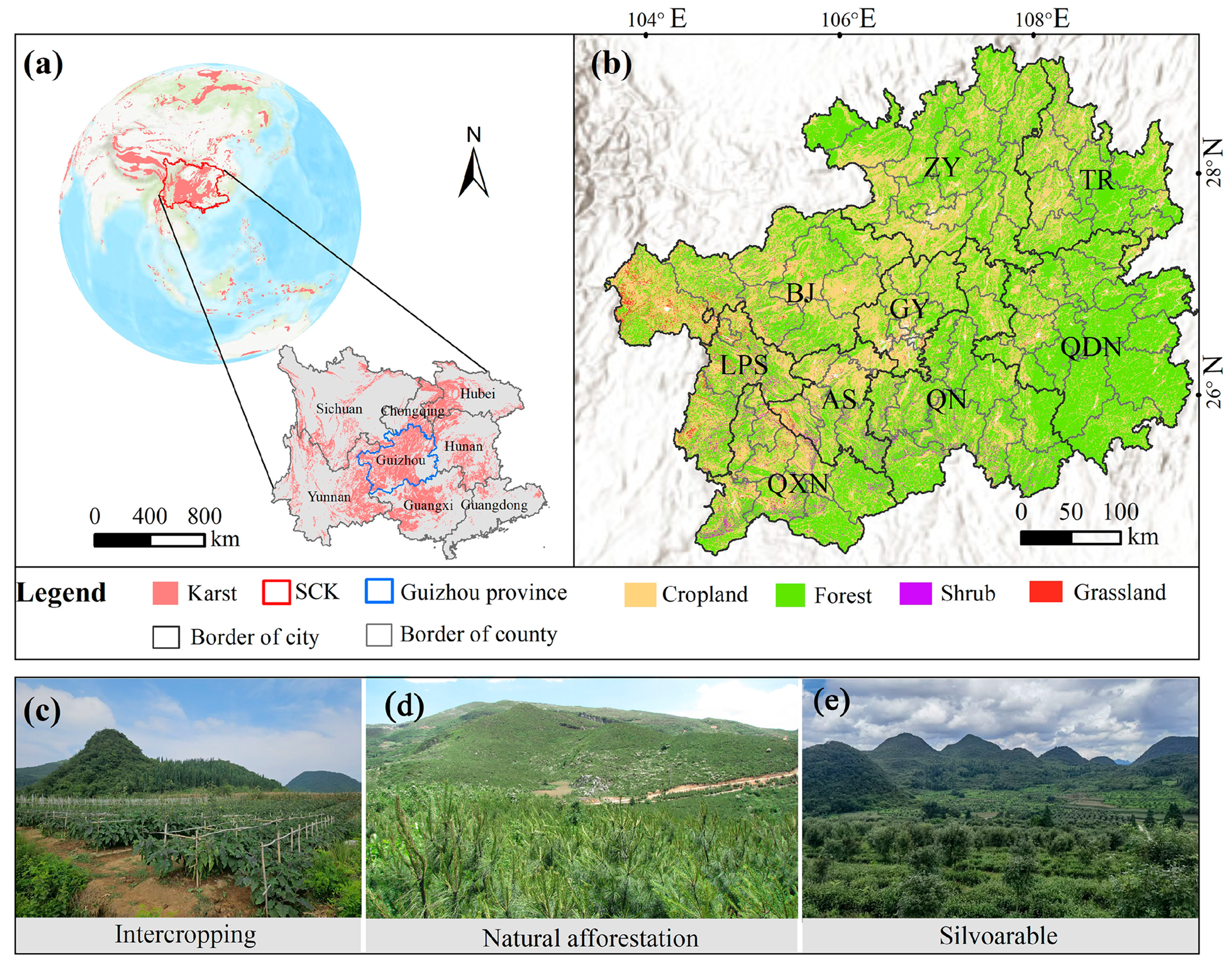
2.1. Study Area

Guizhou Province (24°30′–29°13′ N, 103°31′–109°30′ E) as the core area of the SCK, one of the world’s three major karst areas (Figure 1), is located in the southwest of China [41]. With a land area of 176,100 km², the karst area accounts for 73.8% of the total area of the province [54,55]. Here, rich karst landforms have developed, such as karst peak forests, depressions, underground caves, etc. [55]. As the only province in China without plains, it is the most typical karst province in the world [55]. It is mainly mountainous and hilly, with an average annual temperature of about 15 °C and an average annual precipitation of approximately 1200 mm. Soil types mainly include calcareous soil, yellow soil, purple soil and paddy soil. Vegetation types are mainly subtropical evergreen broad-leaved forests such as Cyclobalanopsis glauca and Castanopsis eyrei, coniferous forests such as Pinus massoniana and Cunninghamia lanceolata, and deciduous broad-leaved forests such as Fagus lucida, Quercus acutissima and Liquidambar formosana. It has a typical subtropical monsoon climate. According to statistics from Bulletin of Soil and Water Conservation in Guizhou Province, the area of soil erosion in 2022 was 45,700 km². Soil and water conservation remains a key ecological restoration project. Large-scale restoration measures such as mountain closure for afforestation, returning farmland to forest, converting slopes into terraces and agroforestry have been implemented in the region [56,57]. From 2000 to 2020, the total area of farmland returned to forest (grassland) there was 2.3817 million hectares, of which the area of farmland converted into forest land accounted for 84.86% of the total area of farmland returned to forest (grassland) [56]. The AF ecosystem is typical and representative. Guizhou Province governs 9 cities, including Guiyang (GY), Tongren (TR), Zunyi (ZY), Anshun (AS), Liupanshui (LPS), Qianxinan Prefecture Buyi and Miao Autonomous Prefecture (QXN), Qianxinan Prefecture Buyi and Miao Autonomous Prefecture (QN) and Qianxinan Prefecture Miao and Dong Autonomous Prefecture (QDN), with a total of 88 counties and districts.

2.2. Data Source

The data used in this study include land-use data, soil erosion area data and remote sensing image data from 2010 to 2020 (

Table 1. Data sources. Land surface temperature (LST) refers to the temperature of the Earth’s surface (including the ground, buildings, vegetation, etc.).

Data type	Resolution	Source
Land use	30 m 2010–2020	From paper [58] https://zenodo.org/record/8176941 (accessed on 3 June 2025)
Remote sensing image	TIF image	https://earthengine.google.com/ (accessed on 3 June 2025) MODIS/061/MOD09A1 MODIS/061/MOD13A1 MODIS/061/MOD11A2
	NDVI
	LST
Area of soil erosion	2010, 2015 and 2020	Bulletin of Soil and Water Conservation in Guizhou Province (https://www.guizhou.gov.cn/ (accessed on 3 June 2025))
Administrative boundary	-	National Geomatics Center of China (https://www.ngcc.cn/ (accessed on 3 June 2025))

). Among them, the resolution of the land-use data is 30 m; Huang et al. [58] produced them based on all available Landsat data on Google Earth Engine (GEE), with a total of 5463 visual interpretation samples. The overall accuracy ranged from 76.45% to 82.51%, the average overall accuracy reached 79.3% ± 1.99%, and the water body had the highest accuracy (87.06% ± 7.07%). Then, there was the forest (85.49% ± 1.30%). The remote sensing image data were obtained and processed through the GEE platform. The image acquisition time was from May to September, and the cloud cover was less than 10%.

2.3. Research Framework

This study aims to reveal whether SWCAF can improve RER and how to promote their relationship. We took Guizhou Province as the study area, and the research time was from 2010 to 2020. Firstly, the spatial and temporal changes in AF, SWL, AFESV and REEQ were analyzed. Then, the methods of Spearman correlation and bivariate spatial autocorrelation were employed to reveal the trade-off–synergy relationship between the AFESV and RER; finally, we used the PVAR model to further verify the relationship between them. The research framework is shown in Figure 2.

2.4. Research Method

2.4.1. Quantification of AFESV

The AFESV was calculated by referring to the improved value equivalent scale by Xie et al. [48]. According to the land-use status in Guizhou Province, AF is classified into cultivated land (including paddy fields and dry land), forest land (including natural forests, economic forests, orchards, tea gardens, etc.), shrubs and grassland. Firstly, we calculated the value coefficient of one equivalent based on the 1/7 formula [59]. We collected data on the sown area, the yield per unit area and the unit price of agricultural products from 2010 to 2020 through the “Compilation of Agricultural Product Cost and Benefit Data”. To avoid fluctuations in the ESV equivalent caused by different grain selling prices in different years, referring to the relevant research by Zhou et al. [60], the annual average value coefficient of the research period was taken as the final value coefficient. According to Formula (1), the value coefficient of one equivalent in the study area was calculated to be 1561.91 CNY/hm². Then, on this basis, the revised service value coefficient was calculated (

Table 2. Value coefficient of SWCAF in Guizhou Province.

Type	Ecosystem Service	Cropland	Forest	Shrub	Grassland
Provision service (PSV)	Food production	1327.62	452.95	296.76	156.19
	Materials production	624.76	1030.86	671.62	218.67
	Water resource supply	31.24	531.05	343.62	124.95
Regulation service (RSV)	Gas regulation	1046.48	3389.35	2202.29	796.57
	Climate regulation	562.29	10,152.42	6606.88	2092.96
	Purification of environment	156.19	3014.49	1999.25	687.24
	Hydrological regulation	421.72	7403.46	5232.40	1530.67
Support service (SSV)	Soil conservation	1608.77	4139.06	2686.49	968.38
	Nutrient cycle	187.43	312.38	203.05	78.10
	Biodiversity	203.05	3764.21	2452.20	874.67
Cultural service (CSV)	Aesthetic landscape	93.71	1655.63	1077.72	390.48

). Finally, based on Table 2 and the area of agroforestry, we calculated the ESV of each county and district in Guizhou Province from 2010 to 2020.

$$VC={\displaystyle \frac{1}{7}}{\sum }_{i=1}^n{p}_i{q}_i{d}_i / S$$

(1)

In Formula (1), VC is an equivalent standard value coefficient (CNY/hm²), and d, p, and q are the sown area (hm²), the unit price (yuan/t⁻¹), and the yield per unit area (kg/hm²) of agricultural products, respectively. Agricultural products include rice, corn, and wheat, and S is the total sown area (hm²) of these agricultural products.

$${VE}_{ij}=C_{ij}VC$$

(2)

In Formula (2), VE_ij represents the value coefficient (CNY/hm²) of the j service function of the i ecosystem, and C_ij is the standard equivalent factor of the j service function of the i ecosystem.

$$ESV={\sum }_{i=0}^n({LUC}_i\times {VC}_i)$$

(3)

In Formula (3), ESV represents the value of ecosystem services (CNY billion), LUC_i represents the area of Class i ecosystems (hm²), and VC_i represents the value coefficient of the service functions corresponding to Class i ecosystems (yuan/hm²).

2.4.2. Quantification of RER

The level of RER was evaluated by using SWL and rural ecological environment quality (REEQ). Among them, SWL is classified into different grades with reference to the current standard classification [61]; according to the average soil erosion modulus (t/km² a) and the average loss thickness (mm/a), we divide SWL into five degrees: mild loss, moderate loss, strong loss, very strong loss and severe loss. Mild loss and severe loss refer to the best and worst statuses of SWL, respectively. In this study, the data on SWL from the Bulletin of Soil and Water Conservation in Guizhou Province refer to the areas of soil erosion, and the unit is m². The RSEI is based on the theory of ecosystem integrity and objectively assesses the regional ecological environment quality by combining multiple ecological indicators, such as NDVI, WET, NDBSI and LST. The model is easier to obtain and facilitates the rapid assessment of the ecological environment status [62,63]. The rock exposure rate and the ecological sensitivity are high in karst areas [64], and the traditional RSEI may underestimate the impact of bare rock on ecology. Including the NDRI in the RSEI to form the KRSEI can represent the changes in ecological factors accurately, with strong accuracy and applicability [65]. So, to enhance the applicability of the RSEI in karst areas, in this study, the normalized differential rocky index (NDRI) was incorporated into the RSEI model, and the karst remote sensing ecological index (KRSEI) model was constructed to evaluate REEQ. The NDRI was calculated by referring to a method in existing research [65]. The Supplementary Materials show the calculation formulas of each index of the KRSEI (see Table S1 for the formulas).

$${KRSEI}_0={PC}_1\left(NDVI,WET,NDBSI,LST,NDRI\right)$$

(4)

$$REEQ=({KRSEI}_0-{KRSEI}_{0min})/({KRSEI}_0-{KRSEI}_{0max})$$

(5)

In the above formula, KRSEI₀ represents the first principal component result after the principal component analysis of the NDVI, WET, NDBSI, LST and NDRI indicators. The value of REEQ is between 0 and 1, dividing it into five grades, namely, I (0–0.2), II (0.2–0.4), III (0.4–0.6), IV (0.6–0.8) and V (0.8–1), using the equally spaced classification method. The higher the grade, the better the ecological environment quality.

2.4.3. Trade-Off–Synergy Analysis

Spearman correlation coefficient analysis was used to represent the trade-off–synergy relationship among the AFESV, REEQ and SWL. The correlation coefficient is within the range of [−1, 1]. When the coefficient is greater than 0, it indicates that there is a synergy effect among the variables; otherwise, it indicates that there is a trade-off effect.

The spatial correlation among AFESV, REEQ and SWL was determined by using bivariate global spatial autocorrelation and local spatial autocorrelation [66], calculated with Geoda v1.22.

$$\mathrm{I}={\displaystyle \frac{\mathrm{n}}{{\sum }_{\mathrm{i}}^{\mathrm{n}}{\sum }_{\mathrm{j}=1}^{\mathrm{n}}{\mathrm{W}}_{\mathrm{ij}}}}{\displaystyle \frac{{\sum }_{\mathrm{i}}^{\mathrm{n}}{\sum }_{\mathrm{j}=1}^{\mathrm{n}}{\mathrm{W}}_{\mathrm{ij}}({\mathrm{x}}_{\mathrm{i}} - \stackrel{\_}{\mathrm{x}})({\mathrm{x}}_{\mathrm{j}} - \stackrel{\_}{\mathrm{x}})}{{{\sum }_i({\mathrm{x}}_{\mathrm{i}} - \stackrel{\_}{\mathrm{x}})}^2}}$$

(6)

$${\mathrm{I}}_{\mathrm{x}}={\displaystyle \frac{({\mathrm{x}}_{\mathrm{i}} - \stackrel{\_}{\mathrm{x}})}{\frac{1}{\mathrm{n}}{{\sum }_i({\mathrm{x}}_{\mathrm{i}} - \stackrel{\_}{\mathrm{x}})}^2}}{\mathrm{W}}_{\mathrm{ij}}({\mathrm{x}}_{\mathrm{j}} - \stackrel{\_}{\mathrm{x}})$$

(7)

In the above formula, I represent the global Moran’s I, with a value range of [−1,1]. If Moran’s I > 0, it indicates a positive correlation in space; otherwise, it indicates a negative correlation in space [67]. I_x stands for the local Moran’s I. Local spatial autocorrelation generates the Local Indicators of Spatial Association (LISA) map [68], in which the clustering types include high–high clustering, low–low clustering, high–low clustering and low–high clustering. In this study, the high–high and low–low accumulations indicate the existence of a synergy relationship between the two variables, while the high–low and low–high accumulations suggest the existence of a trade-off relationship.

2.4.4. PVAR Model Analysis

The panel vector autoregressive (PVAR) model can effectively solve the problem of individual heterogeneity by using panel data, fully considering the individual effect and the time effect. Therefore, it can capture the dynamic relationship between data more accurately and is often used in the study of the interaction relationship between variables [69]. The PVAR model was used to analyze the relationship between SWCAF and RER. We set the AFESV and REEQ from 2010 to 2020 as the model variables. Firstly, we conducted unit root and cointegration tests on the data. If necessary, we used the first-order difference to flatten the data. Then, we run the Granger causality test, impulse response and variance decomposition program to explain the causal relationship and response degree among the variables. The entire process was run by using the PVAR2 package in Stata v18.0 [70]. The theoretical formula of the PVAR model is

$$Y_{it}={\beta }_0+{\sum }_{j=1}^p{\alpha }_j{Y}_{it-j}+f_j+d_t+e_{it}$$

(8)

In Equation (8), Y_it is the column vector of the AFESV and REEQ, that is, the endogenous variable of County i in year t; β₀ is the intercept term; j is the lag order; α_j is the regression coefficient matrix; Y_it-j are all endogenous variables; f_j is the fixed effect; d_t is the time effect; and e_it represents the random error.

The data for panel vector autoregression must be stationary and have a cointegration relationship [71]. Therefore, multiple models, such as IPS, ADF and PP, are adopted to detect whether there are unit roots in the data, in order to avoid the errors caused by a single method [72]. The Pedroni, Kao and Westerlund tests were used to test whether there was a long-term cointegration relationship among the variables. In addition, to ensure the validity and degree of freedom of the estimated parameters, the optimal lag order of the PVAR model was selected based on the information minimization criterion. The three information criterion values of AIC, BIC and HQIC were calculated for the models lagging by 1–4 orders. The optimal lag order of the model is determined by the minimum value of the combination of these three information criterion values [73].

2.4.5. Geo-Informatic Tupu Method

Geo-informatic Tupu is widely applied in the field of spatial information changes, as it can visually reflect the process information, spatial information and attribute information of changes, especially land-use changes [74]. According to an existing study [75], the change map of SWCAF was established, coding cropland, forest, shrubs and grassland as 1, 2, 3 and 4. We took the type of the AF subsystem of the previous period as the tens digit and the subsequent period as the unit digit. We performed calculations according to Formula (9) to generate the change graph of AF over a period of time.

$$N=10A+B$$

(9)

In Formula (9), N represents the newly generated agroforestry change code, A is the type of the initial agroforestry subsystem, and B is the type of the final agroforestry subsystem.

3. Results

3.1. Changes in SWCAF and SWL

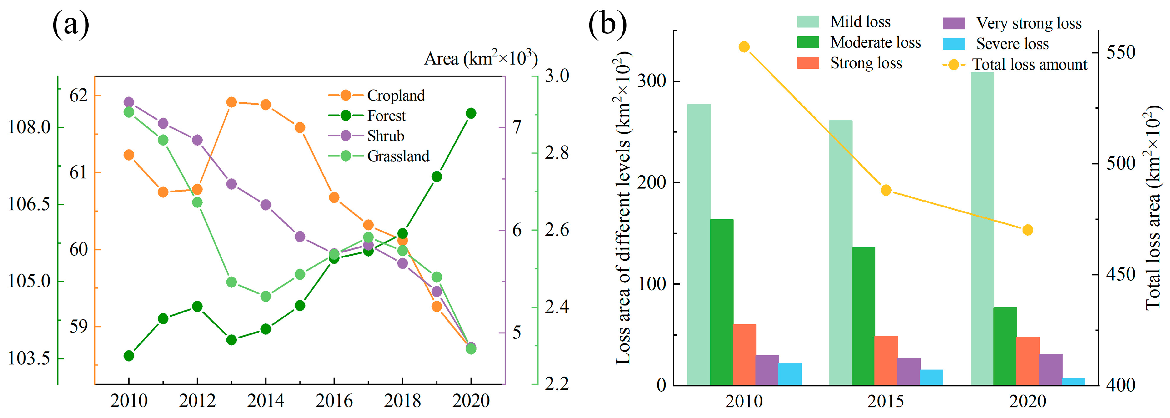
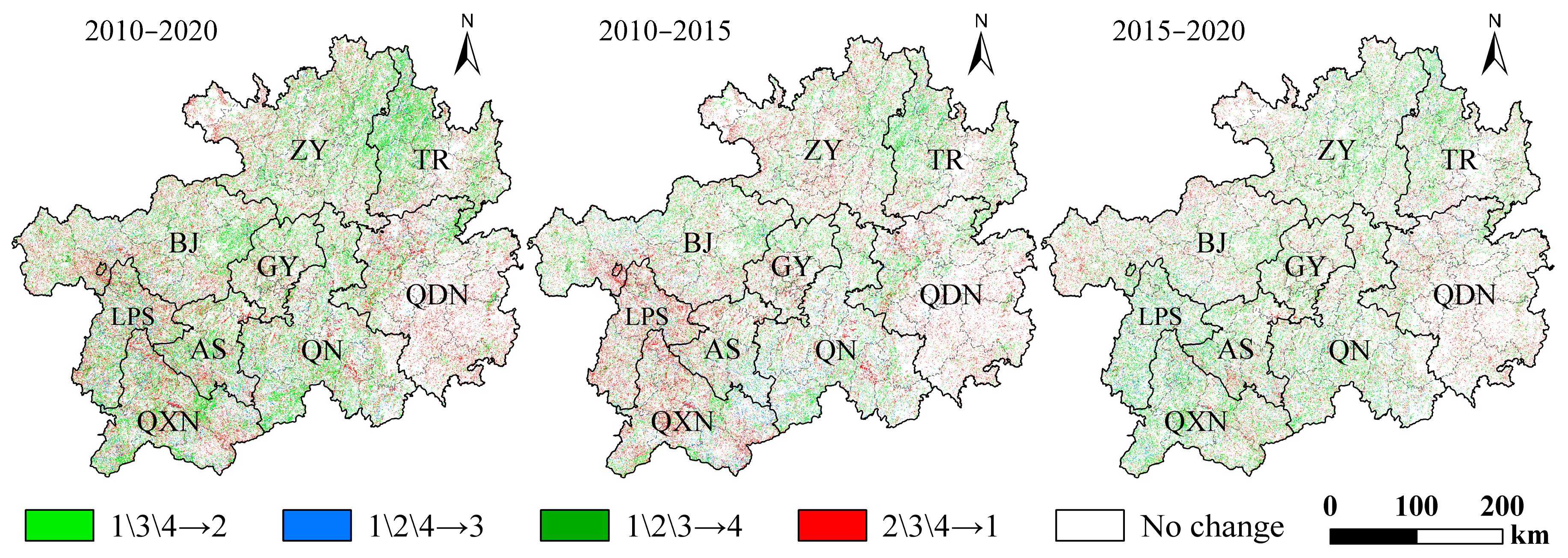
3.1.1. Changes in SWCAF Areas

From 2010 to 2020, the area of AF decreased by 798.333 km² in total (Figure 3; see Table S2 for AF area statistics). The cropland area showed a fluctuating decreasing trend, reaching the maximum in 2015. Over the 11 years, the total reduction area was 2516.286 km². Shrubs continued to decrease, with a reduction area of 2387.122 km², and grassland decreased by 614.807 km². On the contrary, the forest area showed an upward trend, increasing by a total of 4719.881 km² over 11 years, with a growth rate of 4.56%. From the perspective of the transfer directions of different subsystems, during the period from 2010 to 2020, the transfer areas of cropland, shrub and grassland to forests were the largest, totaling 11,549.07 km² and being mainly distributed in the northern, southern and western parts of Guizhou Province, while the change in QDN was not obvious (Figure 4; see Table S3 for AF area change statistics). Among them, cropland accounted for 75.71% and was the largest contributor to the shift to forests, followed by shrubs (20.07%). In addition, other subsystems also transformed into shrubs, grassland and cultivated land. The total area converted into cultivated land amounted to 8345.435 km², which was the second largest type of transformation after forests. From the perspective of different time periods, from 2010 to 2015, the area of cropland, shrub and grassland transferred to forests was 6405.44 km². Among them, in terms of the transfer proportion, the order was cropland (77.75%), shrubs (18.85%) and grassland (3.4%). This transformation was mainly concentrated in regions such as TR, BJ, QN and AS. During this period, there was also an obvious transfer of other subsystems to cropland, with a total area of 6714.386 km². From 2015 to 2020, the area transferred to forests further increased, totaling 7606.682 km², while the area transferred to cultivated land decreased, totaling 4436.029 km².

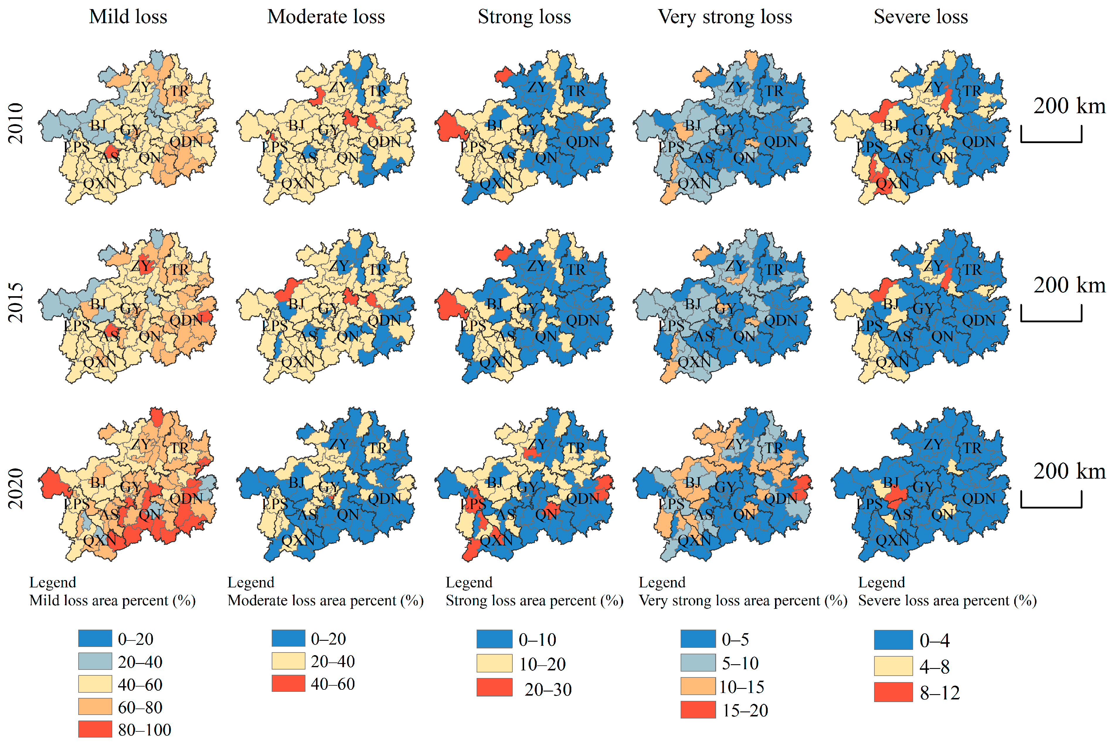
3.1.2. Changes in SWL Areas

From 2010 to 2020, the SWL area in Guizhou Province showed an obvious downward trend. The total SWL area decreased from 55,258.18 km² to 47,008.2 km², a reduction of 14.93%, over 11 years (Figure 3). From the perspective of the composition of different degrees of loss, Guizhou Province mainly experienced mild loss and moderate loss. The sum of their areas accounted for 79.71%, 81.38% and 81.86% of the total area of SWL in 2010, 2015 and 2020, respectively. Compared with 2010, the area of mild erosion decreased by 1588.52 km² in 2015 but increased by 3133.09 km² in 2020. The area of other degrees mostly showed a continuous decline. The area of moderate loss decreased by 8701.29 km², that of severe erosion decreased by 1225.15 km², and that of intense erosion decreased by 1565.63 km², while the area of extremely severe erosion increased by 109 km², which accounted for only a very small part. In 2010, the degrees of soil erosion in various districts and counties were mainly mild and moderate erosion, and the same characteristics were observed in 2015 (Figure 5). During these two periods, the number of counties and districts with a moderate erosion area proportion of 20%–40% was comparable, distributed in areas where forests, shrubs and grassland were transferred to cultivated land, such as LPS, QN and ZY. However, in 2020, this number decreased obviously, which may reveal that the expansion of cultivated land area is not conducive to SWC. The forest ecosystem mainly composed of trees can effectively control soil erosion. In 2020, the proportion of areas with moderate and severe loss decreased obviously, while the proportion of areas with mild loss increased further.

3.2. Changes in ESV and REEQ

3.2.1. Changes in Total ESV

From 2010 to 2020, the total ESV showed an upward trend, increasing by CNY 9.1813 billion, an increase of 2.14% compared with 2010 (

Table 3. Changes in total ESV from 2010 to 2020.

	ESV (CNY 108)			Change Rate (%)
	2010	2015	2020	2010–2020	2010–2015	2015–2020
Cropland	383.486	385.723	367.726	−4.11%	0.58%	−4.67%
Forests	3712.071	3747.028	3881.259	4.56%	0.94%	3.58%
Shrubs	172.263	141.147	115.516	−32.94%	−18.06%	−18.16%
Grassland	23.019	19.682	18.151	−21.15%	−14.50%	−7.78%
Total ESV	4290.839	4293.579	4382.652	2.14%	0.06%	2.07%

). From the perspective of changes in different periods, the ESV grew relatively little from 2010 to 2015, while it grew the most and the fastest from 2015 to 2020, with total changes of CNY 274 million and CNY 8.9073 billion, respectively. The source of the ESV in Guizhou Province is mainly based on forests, followed by cultivated land, shrubs and grassland. From 2010 to 2020, only the ESV of forests increased, reaching CNY 16.9188 billion, with an increase rate of 4.56%, contributing 184% to ESV. From 2015 to 2020, the increase rate was the highest, reaching 3.58%. The ESV of shrubs, grassland and cultivated land decreased by CNY 5.6747 billion, CNY 486.8 million and CNY 1.576 billion, respectively, with the former two having the greatest reduction.

The ESV shows a trend of increase in the west and decrease in the east (Figure 6). The increase was obvious in ZY, TR and other places, while the decrease was obvious in various districts and counties of QDN. From the perspective of different research periods, the increase in value from 2010 to 2015 was mainly concentrated in a few areas in the north and south of Guizhou Province. From 2015 to 2020, the area of increasing value further expanded, but the QDN area still showed a decreasing trend.

3.2.2. Changes in Individual ESVs

Among the individual ESVs, except food production and hydrological regulation services, all showed linear growth (

Table 4. Individual ESVs from 2010 to 2020.

Single ESV	Year			Variation (CNY 108)
	2010	2015	2020	2010–2020	2010–2015	2015–2020
Food production	130.798	131.26	128.791	−2.007	0.462	−2.469
Materials production	150.508	150.765	152.064	1.556	0.257	1.299
Water resource supply	59.76	59.785	61.29	1.531	0.027	1.504
Gas regulation	433.338	433.797	440.954	7.617	0.461	7.157
Climate regulation	1139.737	1140.308	1169.182	29.445	0.571	28.874
Purification of environment	338.218	338.307	346.858	8.640	0.089	8.551
Hydrological regulation	834.862	834.739	855.313	20.451	−0.124	20.574
Soil conservation	549.411	550.097	557.89	8.479	0.686	7.793
Nutrient cycle	45.523	45.596	45.994	0.470	0.073	0.397
Biodiversity	422.552	422.717	433.417	10.864	0.165	10.699
Aesthetic landscape	186.133	186.206	190.899	4.766	0.073	4.693

). Food production services decreased by CNY 246.9 million between 2015 and 2020, and hydrological regulation services decreased by CNY 12.4 million between 2010 and 2015. Among the individual ESVs that increased linearly, the service with the largest increment was climate regulation, with its value increasing by CNY 2.9445 billion during the research period. Then, there were services such as biodiversity and environmental purification, which increased by CNY 1.0864 billion and CNY 864 million, respectively. The value of soil conservation services increased by CNY 847.9 million, with the largest increase from 2010 to 2020, representing a 1.4% increase compared with 2015.

3.2.3. Changes in REEQ

During the study period, the mean value of the KRSEI increased from 0.691 to 0.703, indicating a certain improvement in REEQ in Guizhou Province (Figure 7). The overall distribution pattern of REEQ is low values in the west and high values in the east. Over the past 11 years, there was an obvious improvement in the western part of Guizhou, while the eastern part slightly deteriorated. This spatial distribution pattern has certain similarities to the AFESV in terms of spatial distribution, indicating that SWC measures such as afforestation and mountain closure for afforestation have promoted the improvement in REEQ. From the perspective of the proportion of different ecological grades, grades IV and V were dominant, accounting for 56.66% and 24.02%, respectively, in 2020. From 2010 to 2020, grades I to III showed a fluctuating downward trend, while grades IV and III rose. Compared with 2010, the area of grades IV increased by 18.14%. In summary, the overall REEQ in Guizhou Province shows an improving trend, especially in the key areas of SWC in the west. Meanwhile, the ecological grade is developing towards a higher grade, and the ecological grade structure is constantly being optimized.

3.3. The Trade-Off–Synergy Relationship Between AFESV and RER

3.3.1. Spearman Correlation Analysis

During the study period, there was an obvious positive correlation between REEQ and the AFESV (r = 0.6, p < 0.05), and the correlation gradually increased over time (Figure 8). This indicates that there is an obvious synergistic relationship between the AFESV and REEQ, and the promoting effect between the two is strengthening. From 2010 to 2020, the trade-off relationship between the AFESV and REEQ mainly emerged among the NDBSI, the NDRI and other ecosystem services. There is a trade-off relationship between PSV and WET, LST, NDBSI and NDRI, indicating that excessive absorption of food supply and water supply over a long period of time is not conducive to the increase in surface moisture and the prevention and control of bare rock soil. In 2020, there was an obvious synergistic relationship between RSV, SSV and CSV and the KRSEI, specifically manifested as the promoting effect on the NDVI, WET and LST. The area of soil erosion is another important indicator representing the level of rural revitalization in karst areas. The correlation results show that there is an obvious positive correlation between SWL and ESV (r = 0.69, p < 0.05). From 2010 to 2020, the correlation coefficient increased by 0.03, indicating that the continuous increase in agroforestry ecosystem services is conducive to soil erosion control. In 2020, PSV, RSV, SSV and CSV were all positively correlated with SWL, and the correlation value of the PSV was the largest at 0.81, followed by the SSV at 0.7, indicating that they are key factors in controlling soil erosion.

3.3.2. Bivariate Spatial Autocorrelation

The Moran’s I values among the AFESV, REEQ and SWL are all greater than 0, indicating an obvious spatial positive correlation among them (see Figure S1 for the Moran’s I). From 2010 to 2020, the Moran’s I value became larger and larger, indicating that the spatial correlation became stronger and stronger. The results of local spatial autocorrelation show that the spatial relationship between the AFESV and REEQ is mainly characterized by high–high and low–low accumulations. The low–low accumulation is distributed in AS, Guiyang, QN, etc., and the high–high accumulation is distributed in QDN, TR, etc. (Figure 9; see Figure S2 for the significance), indicating that there is a synergistic relationship between the AFESV and REEQ in these areas. The low–high and low–low accumulations indicate the trade-off relationship between the two and are mainly distributed in LPS and the eastern part of GY, gradually decreasing with time. The low–low accumulation is also shrinking. This indicates that the development of REER and the AFESV is gradually coordinating, and the promoting effect of agroforestry on ecology is gradually emerging. From 2010 to 2020, the AFESV and SWL were also mainly characterized by high and low accumulations, and the changes over time were not obvious (Figure 9). It is indicated that there is a long-term and stable synergy relationship between the AFESV and SWL. Agroforestry can curb soil erosion to a certain extent and improve rural ecology.

3.4. Interaction Between SWCAF and RER Based on PVAR Model

3.4.1. Variable Stability

The results show that during the period from 2010 to 2020, both the AFESV and RER rejected the null hypothesis at the 1% level, indicating that the variables passed the unit root test and the data were stationary on the time series (see Table S4 for the unit root test). In addition, the variables passed the Kao, Westerlund and Pedroni tests, indicating that there is a long-term equilibrium relationship among the variables (see Table S5 for the unit cointegration test). The above results indicate that the variables AFESV and RER can be further analyzed by the Granger causality test and the PVAR model.

3.4.2. Granger Causality

Table S6 (showing the optimal lag order) shows that the AIC, BIC and HQIC of the model established in this study are the smallest at the fourth order; therefore, it is optimal when lagging by four orders. The results of the Granger causality test show that both the AFESV and RER reject the null hypothesis at the 5% level, indicating that they show mutual Granger causality (see Table S7 for the granger causality).

3.4.3. Impulse Response and Variance Decomposition

Regression analysis can represent the influence relationship between variables, but it cannot analyze the dynamic influence relationship produced when variables are subjected to certain shocks. Impulse response analysis, however, can analyze this dynamic influence. Based on the conclusion of Granger causality, the response intensity and persistence of the AFESV and RER within 10 periods after being subjected to 200 mutual impacts by Monte Carlo were evaluated, and the influence intensity and contribution of the independent variable on the dependent variable were characterized by analysis of variance.

Figure 10 shows the results of the impulse response. The results show that there is a strong nonlinear relationship between the AFESV and RER. From the perspective of the impact of RER and the AFESV on themselves, we found the following: Firstly, the response of RER to itself is positive in the early stage, then drops rapidly, reaches the minimum value in the first stage, shows a negative effect, then turns positive in the second stage and converges to 0 in the ninth stage. This indicates that in the early stage of ecological restoration, the implementation of ecological policies and projects leads to an increase in ecological resources and environmental improvement, effectively enhancing ecological indicators such as soil and water conservation capacity and the NDVI in the short term. But the rapid transformation into negative effects may reveal the disruption of ecological balance and the recovery of ecological pressure caused by economic development activities during the ecological restoration process. Secondly, when the AFESV is impacted by itself, it initially shows the greatest positive effect, maintains a weak positive effect in the fourth stage and converges to 0 in the sixth stage. This indicates that the agroforestry ecosystem has a strong promoting effect on itself. From the perspective of the interaction relationship between RER and the AFESV, we found the following: Firstly, the response of RER to the AFESV is negative in the initial stage, reaches the maximum negative effect in the first stage, turns positive after the second stage and tends to converge to 0 in the tenth stage. Then, after the AFESV is impacted by the RER, it initially shows positive feedback, turns to a negative effect in the first stage, reaches the maximum in the second stage and converges to 0 in the eighth stage. It can be seen from

Table 5. Results of variance decomposition.

Impact Variable	AFESV		RER
Response Variable	RER	AFESV	AFESV	RER
1	0	0.996	0.004	1
2	0.013	0.996	0.004	0.987
3	0.015	0.993	0.007	0.985
4	0.026	0.984	0.016	0.974
5	0.025	0.984	0.016	0.975
6	0.026	0.984	0.016	0.974
7	0.027	0.983	0.017	0.973
8	0.027	0.983	0.017	0.973
9	0.027	0.983	0.017	0.973
10	0.027	0.983	0.017	0.973

that the contribution of the AFESV to itself shows a downward trend and reaches the minimum value of 0.93 in the seventh stage, indicating that compared with RER, the AFESV is mainly affected by itself. The degrees of mutual influence between the AFESV and RER increased over stages and reached the maximum values in the seventh stage, which were 0.027 and 0.017, respectively. It is indicated that the AFESV has an obvious promoting effect on RER and constantly increases over stages.

4. Discussion

4.1. Benefits of SWC in AF

During the research period, the obvious change characteristics of AF were the large-scale transfer of cropland, shrubs and grassland to forests, totaling 11,549.07 km², while the area of SWL decreased by 14.93%. There was an obvious correlation among them. The forest area increased rapidly by 4719.881 km², which might have been driven by policies. In 2003, China implemented the large-scale project of returning farmland to forests. The SCK, as a key area for soil erosion control, also carried out the project of controlling rocky desertification. Especially since 2010, it has strengthened ecological restoration efforts. In 2012, Guizhou Province initiated the project of returning farmland to forests and grassland on its own. This is similar to the research by Yuan et al. [76] and Xu et al. [77]. Their results show that ecological restoration projects such as returning farmland to forests and controlling rocky desertification have obviously changed the land-use type and effectively increased the forest area. Additionally, the increase in the forest coverage rate effectively inhibited soil erosion by enhancing the rainwater interception capacity of surface vegetation and reducing the scouring force of runoff. The areas of moderate, strong and severe erosion decreased by 8701.29 km², 1225.15 km² and 1565.63 km², respectively. The research study by Niu et al. [78] shows that since the implementation of the project of returning farmland to forests, the SWC services at the core of the SCK have shown an obvious upward trend and that this trend is obviously positively correlated with the vegetation coverage rate. In the early stage (2010–2015), a large area of cropland was transferred to forests, 4980.23 km². However, shrubs and grassland also underwent reverse transfers to cropland, which weakened the ecological benefits of agroforestry. As a result, the area of mild erosion temporarily decreased and then rebounded and increased again in the later stage (2015–2020). In this study, the cropland area decreased first and then increased in the early stage. Because in the control of soil erosion, AF models such as under-forest breeding and the intercropping of agriculture and forestry have been actively adopted, which has led to the transformation of some abandoned land, grassland and shrubs into cultivated land [79]. Natural land is unstable after being disturbed by human activities and may lead to an increase in the area of soil erosion in the short term. In the later stage, the area transferred to forests further increased, the area turned into cropland decreased, and the area of severe erosion decreased obviously on a large scale. This is because, during this period, the “Guizhou Province Soil and Water Conservation Plan (2016–2030)” promulgated by Guizhou Province strengthened the implementation of SWC measures and improved the ecological compensation mechanism. The AF changes in the QDN area are not obvious, and the soil erosion grade has long been mainly mild or moderate erosion. This might be because this area belongs to an atypical karst area, the ecosystem is relatively stable and the vegetation is mainly forest. In regions such as BJ, ZY, LPS and QN, the grade of soil erosion has undergone obvious changes, and the area of moderate erosion has decreased obviously. This indicates that SWC engineering measures such as forest restoration, afforestation and grass planting, and mountain closure for afforestation have effectively alleviated soil erosion in these areas. The slight increase in the area of extremely intense erosion may suggest that ecological degradation is caused by the destruction of AF through activities such as urban construction and resource exploitation. Therefore, the increase in forest area in the AF system can effectively control soil erosion, while excessive human interference with AF may weaken the SWC benefits in the short term.

4.2. Changes in AFESV and REEQ

The overall AFESV increased by CNY 9.181 billion. Forests led the increase in value, with a total increase of CNY 16.919 billion. This is similar to the research conclusion by Sun et al. [80]. The contribution of forests to the improvement in the AFESV is related to the large-scale restoration of forests. This actually reflects the long-term effects of measures such as closing mountains for afforestation in AF. The increase in the tree coverage rate can directly enhance the functions of agroforestry ecosystems and improve ecosystem services [81]. The increase in forest area has directly promoted the growth of core ESVs such as climate regulation, hydrological regulation and soil conservation, which increased by CNY 2.945 billion, CNY 2.045 billion and CNY 847.9 million, respectively. However, the decline in the ESV of shrubs, grassland and cultivated land suggests that the restoration of forests may have sacrificed certain services of cropland and shrubbery ecosystems, such as forage supply [82], niche support [83], etc. In particular, the decline in food supply services may lead to an increase in pressure on the livelihood of farmers in some local areas, thereby triggering the wanton plundering of ecological resources and directly disrupting the ecological balance [84]. AF can minimize trade-offs and maximize the synergy of ecosystem services [85]. Therefore, in the process of SWC, it is necessary to pay attention to coordinating the composition of the AF ecosystem, balance the contradiction between ecology and livelihood through the intercropping of forest and grain and under-forest breeding and reduce the risk of ecological structure simplification. In addition, given the obvious role of forest ecosystems in SWC, it is necessary to focus on the trade-off–synergy relationship of forest ecosystem services [86,87]. During the research period, REEQ improved slightly, and the KRSEI rose to 0.703. From the perspective of spatial distribution, the ecological grade in the western region obviously increased, and REEQ obviously improved. The spatial distribution pattern is highly similar to the AFESV, indicating the contribution of AF to the improvement in rural ecology. Changes in land use can lead to changes in the quality of the ecological environment. In particular, the improvement in forest ecological quality plays an important role in maintaining the overall ecological quality of the region [88].

4.3. SWCAF Promotes RER in Karst Areas

The promoting effect of SWCAF on RER is reflected in two aspects. The first is to control SWL, and the second is to improve REEQ. From 2010 to 2020, the AFESV and REEQ showed an obvious synergistic relationship, which gradually strengthened and became more obvious over time. This result confirms that AF directly drives RER by enhancing regulation services and reducing the risk of land degradation [89]. However, the trade-off relationship between the PSV and WET (p = −0.08) reveals the potential conflicts between ecological restoration and agricultural production. For instance, short-term excessive food production can exacerbate water consumption and surface dryness [90]. Therefore, it is necessary to further consider incorporating more trees into farmland to increase shade to coordinate ecological protection and agricultural production. The AFESV and SWL also show a synergistic relationship. This further indicates that AF can increase the surface vegetation coverage through the combination of various plants, reduce the direct impact of rainwater on soil and lower the risk of soil erosion [91]. The results of the bivariate spatial autocorrelation analysis show that the spatial relationship of trade-off–synergy between the AFESV and RER roughly coincides with the regions where SWC and rocky desertification control projects are mainly implemented. This further indicates that AF is correlated with REEQ and SWL in spatial distribution.

The relationship between ESs and rural development is complex [92]. Combining econometric methods with other methods and strengthening the exploration of the coupled coordination characteristics, correlation patterns and spatial heterogeneity of ecosystem services and human well-being are conducive to promoting the understanding of the synergistic improvement process of the two [93]. The results in this study indicate that there was an obvious Granger causal relationship between the AFESV and RER, suggesting a bidirectional interaction relationship between them. Study data from Wang et al. [94] have shown that the coupling and coordination degrees of ESs and rural revitalization in the southeastern Himalayas are lower in early stages but higher in later stages. And the influence of the AFESV on RER is negative in early stages and positive later in our study. This result in our study can be explained by Wang et al. to a certain extent. In karst areas, there is a high demand for population support; in the early stage of the development of AF, more emphasis was placed on food supply [95]. Increasing the supply of AFESs, especially the PSV, in the short term will lead to the deterioration of the rural ecological environment. Because of excessive reclamation, the overuse of chemical fertilizers and pesticides and other behaviors may damage soil structure, reduce biodiversity and pollute water bodies, thereby causing environmental degradation [96]. And expanding cropland to further enhance food supply services is bound to reduce tree cover and increase water consumption at the same time, thereby reducing surface humidity and increasing surface temperature and dryness. Therefore, it is necessary to establish a sound ecological compensation mechanism to help farmers relieve the pressure on their livelihoods, thereby curbing the ecological damage caused by survival needs. After being impacted by RER, the AFESV first showed a positive response, which then turned to a negative response. This indicates that RER is beneficial to the development of AF in the early stage, but it may pose a threat in the long term. The essence of RER is a process of improving REEQ. In karst areas, the focus is on carrying out the work of controlling soil erosion. Projects such as returning farmland to forests, converting slopes into terraces and closing mountains for afforestation increase the stock of trees by implementing SWC measures such as planting trees and grass and closing mountains. In the initial stage, it does increase the regulation and support services of AF, but in the long run, it reduces the arable land resources. It is not conducive to the improvement in the PSV. This is similar to the research by Zhong et al. [97]; that is, the synergy–trade-off relationship of ESs under the implementation of ecological restoration projects shows phased differences. The variance decomposition results show that the influence of the AFESV on RER is greater than that of RER on its own and that this influence increases over time. Therefore, in ecological restoration and soil and water management in karst areas, more attention should be paid to the role of AF in improving rural ecology, the internal structure of AF should be coordinated, and trade-offs among services should be avoided as much as possible.

4.4. Limitations

The evaluation of RER is a complex process involving multiple aspects. In this study, based on regional characteristics, the area of SWL and REEQ indicators can reflect the ecological revitalization level in karst villages to a certain extent. However, in the future, more indicators based on available ecological remote sensing technology need to be developed to establish a comprehensive and all-round evaluation system for rural ecology and improve the refinement of the evaluation. Additionally, although AF as an NbS can promote RER according to our study, it is significant to enhance the empirical reliability of the RER indicator and avoid pure model speculation on the relationship of AF and RER by testing different NbSs or including socio-economic survey data in future study. It also necessary to explore more effective NbSs and the gap in AF in ecological restoration in karst areas in the future.

5. Conclusions

This research study takes Guizhou Province, a core karst area in the SCK, as an example and revealed the SWC benefits of SWCAF from 2010 to 2020, as well as the spatio-temporal variations in the AFESV and RER through the equivalent factor method and the KRSEI. Based on correlation analysis and the PVAR model, the interaction between the AFESV and RER was explained. This study found the following: (1) From 2010 to 2020, the area of SWCAF underwent obvious changes. A large area of cropland, shrubs and grassland turned into forests, totaling 11,549.07 km², while the area of soil erosion decreased by 14.93%. The obvious spatial and temporal correlations among them indicate that SWCAF effectively curbed soil erosion. (2) The AFESV increased by CNY 9.181 billion in total, and the ESV of forests increased by CNY 16.919 billion, making it the main contributor. Overall, REEQ shows a slight improvement, and the ecological grade obviously improved. The changes in the AFESV and RER have a similar spatial distribution pattern, mainly characterized by obvious improvement in the areas where farmland is returned to forest and rocky desertification control in the west. (3) The AFESV showed obvious synergistic relationships with REQQ (r = 0.6, p < 0.05) and SWL (r = 0.69, p < 0.05). These synergistic relationships were spatially correlated, and the synergy strengthened over time, indicating that the promoting effect of AF on soil erosion and the quality of the rural ecological environment was gradually strengthening. (4) There is an obvious Granger causal relationship between the AFESV and RER, and the two have alternating positive and negative influences.

This study holds that there is a two-way promoting relationship between SWCAF and RER, and SWCAF has indeed improved the level of RER in Guizhou Province, which is reflected in two aspects: the control of soil erosion and the increase in REEQ. In particular, the forest ecosystem plays a key role in this improvement. However, future work needs to pay attention to the internal structure composition of agriculture and forestry to avoid the trade-offs of ecosystem services caused by the simplification of the structure, which hinders ecological restoration and the realization of human well-being. In addition, the KRSEI constructed in this study represents REEQ. In the future, it can be further applied in research on RER in karst mountains, because this assessment model based on remote sensing technology has the characteristics of convenience and efficiency and can overcome the problem of rough evaluation results caused by the high heterogeneity of karst mountains. In order to improve ecological environment furtherly, it seems to consider more about (i) prioritizing AF systems on steep terrain, (ii) providing compensation to farmers who convert cropland, and (iii) establishing annual monitoring with the remote sensing of the AFESV and RER to further improve ecological restoration in karst areas. This study helps promote global ecological restoration, providing a feasible reference for decision making and the management of soil and water conservation in the SCK and even global karst areas. The method proposed in this study can serve as a reference guide for the restoration of karst ecosystems in other climate zones, such as the Mediterranean, in Europe, and Yucatan, Mexico.

References

1. Lal, R. Soil erosion and the global carbon budget. Environ. Int. 2003, 29, 437–450. [Google Scholar] [CrossRef] [PubMed]
2. Wynants, M.; Kelly, C.; Mtei, K.; Munishi, L.; Patrick, A.; Rabinovich, A.; Nasseri, M.; Gilvear, D.; Roberts, N.; Boeckx, P.; et al. Drivers of increased soil erosion in East Africa’s agro-pastoral systems: Changing interactions between the social, economic and natural domains. Reg. Environ. Change 2019, 19, 1909–1921. [Google Scholar] [CrossRef]
3. Wang, K.L.; Zhang, C.H.; Chen, H.S.; Yue, Y.M.; Zhang, W.; Zhang, M.Y.; Qi, X.K.; Fu, Z.Y. Karst landscapes of China: Patterns, ecosystem processes and services. Landsc. Ecol. 2019, 34, 2743–2763. [Google Scholar] [CrossRef]
4. McDonald, R.I.; Chaplin-Kramer, R.; Mulligan, M.; Kropf, C.M.; Huelsen, S.; Welker, P.; Poor, E.; Erbaugh, J.T.; Masuda, Y.J. Win-wins or trade-offs? Site and strategy determine carbon and local ecosystem service benefits for protection, restoration, and agroforestry. Front. Environ. Sci. 2024, 12, 1432654. [Google Scholar] [CrossRef]
5. Nair, P.K.R. Classification of agroforestry systems. Agrofor. Syst. 1985, 3, 97–128. [Google Scholar] [CrossRef]
6. Wiersum, K. Forest gardens as an ‘intermediate’ land-use system in the nature-culture continuum: Characteristics and future potential. In New Vistas in Agroforestry; Springer: Dordrecht, The Netherlands, 2004. [Google Scholar]
7. Zomer, R.J.; Trabuco, A.; Coe, R.; Place, F.; Noordwijk, M.; Xu, J. Trees on Farms: An Update and Reanalysis of Agroforestry’s Global Extent and Socio-Ecological Characteristics; Working Paper 179; World Agroforestry Centre (ICRAF) Southeast Asia Regional Program: Bogor, Indonesia, 2014. [Google Scholar]
8. Hu, W.M.; Gu, Z.K.; Xiong, K.N.; Lu, Y.R.; Li, Z.J.; Zhang, M.; You, L.H.; Ruan, H. A Review of Value Realization and Rural Revitalization of Eco-Products: Insights for Agroforestry Ecosystem in Karst Desertification Control. Land 2024, 13, 1888. [Google Scholar] [CrossRef]
9. Shin, S.; Soe, K.T.; Lee, H.; Kim, T.H.; Lee, S.; Park, M.S. A systematic map of agroforestry research focusing on ecosystem services in the Asia-Pacific Region. Forests 2020, 11, 368. [Google Scholar] [CrossRef]
10. Jose, S. Agroforestry for ecosystem services and environmental benefits: An overview. Agrofor. Syst. 2009, 76, 1–10. [Google Scholar] [CrossRef]
11. Chidozie, B.C.; Ramos, A.L.; Ferreira, J.V.; Ferreira, L.P. Residual agroforestry biomass supply chain simulation insights and directions: A systematic literature review. Sustainability 2023, 15, 9992. [Google Scholar] [CrossRef]
12. Dollinger, J.; Jose, S. Agroforestry for soil health. Agrofor. Syst. 2018, 92, 213–219. [Google Scholar] [CrossRef]
13. Udawatta, R.P.; Rankoth, L.M.; Jose, S. Agroforestry and biodiversity. Sustainability 2019, 11, 2879. [Google Scholar] [CrossRef]
14. Nair, P.K.R.; Mohan, K.B.; Nair, V.D. Agroforestry as a strategy for carbon sequestration. J. Plant Nutr. Soil Sci. 2009, 172, 10–23. [Google Scholar] [CrossRef]
15. Kaushal, R.; Mandal, D.; Panwar, P.; Kumar, P.; Tomar, J.M.S.; Mehta, H. Soil and water conservation benefits of agroforestry. In Forest Resources Resilience and Conflicts; Elsevier: Amsterdam, The Netherlands, 2021; pp. 259–275. [Google Scholar] [CrossRef]
16. Fahad, S.; Chavan, S.B.; Chichaghare, A.R.; Uthappa, A.R.; Kumar, M.; Kakade, V.; Pradhan, A.; Jinger, D.; Rawale, G.; Yadav, D.K.; et al. Agroforestry systems for soil health improvement and maintenance. Sustainability 2022, 14, 14877. [Google Scholar] [CrossRef]
17. Garrity, D.P.; Akinnifesi, F.K.; Ajayi, O.C.; Weldesemayat, S.G.; Mowo, J.G.; Kalinganire, A.; Larwanou, M.; Bayala, J. Evergreen Agriculture: A robust approach to sustainable food security in Africa. Food Secur. 2010, 2, 197–214. [Google Scholar] [CrossRef]
18. Udawatta, R.P.; Jose, S. Agroforestry strategies to sequester carbon in temperate North America. Agrofor. Syst. 2012, 86, 225–242. [Google Scholar] [CrossRef]
19. Jinger, D.; Kumar, R.; Kakade, V.; Dinesh, D.; Singh, G.; Pande, V.C.; Bhatnagar, P.R.; Rao, B.K.; Vishwakarma, A.K.; Kumar, D.; et al. Agroforestry for controlling soil erosion and enhancing system productivity in ravine lands of Western India under climate change scenario. Environ. Monit. Assess. 2022, 194, 267. [Google Scholar] [CrossRef]
20. Costanza, R.; d’Arge, R.; de Groot, R.; Farber, S.; Grasso, M.; Hannon, B.; Limburg, K.; Naeem, S.; O’Neill, R.V.; Paruelo, J.; et al. The value of the world’s ecosystem services and natural capital. Nature 1997, 387, 253–260. [Google Scholar] [CrossRef]
21. Olschewski, R.; Tscharntke, T.; Benítez, P.C.; Schwarze, S.; Klein, A.M. Economic evaluation of pollination services comparing coffee landscapes in Ecuador and Indonesia. Ecol. Soc. 2006, 11, 7. [Google Scholar] [CrossRef]
22. Tsonkova, P.; Quinkenstein, A.; Böhm, C.; Freese, D.; Schaller, E. Ecosystem services assessment tool for agroforestry (ESAT-A): An approach to assess selected ecosystem services provided by alley cropping systems. Ecol. Indic. 2014, 45, 285–299. [Google Scholar] [CrossRef]
23. Kearney, S.P.; Fonte, S.J.; García, E.; Siles, P.; Chan, K.M.A.; Smukler, S.M. Evaluating ecosystem service trade-offs and synergies from slash-and-mulch agroforestry systems in El Salvador. Ecol. Indic. 2019, 105, 264–278. [Google Scholar] [CrossRef]
24. Leroux, L.; Clermont-Dauphin, C.; Ndienor, M.; Jourdan, C.; Roupsard, O.; Seghieri, J. A spatialized assessment of ecosystem service relationships in a multifunctional agroforestry landscape of Senegal. Sci. Total Environ. 2022, 853, 158707. [Google Scholar] [CrossRef] [PubMed]
25. Ran, R.; Hua, L.; Xiao, J.F.; Ma, L.; Pang, M.Y.; Ni, Z.X. Can poverty alleviation policy enhance ecosystem service value? Evidence from poverty-stricken regions in China. Econ. Anal. Policy 2023, 80, 1509–1525. [Google Scholar] [CrossRef]
26. Ketema, H.; Wei, W.; Legesse, A.; Zinabu, W.; Temesgen, H.; Yirsaw, E. Ecosystem service variation and its importance to the wellbeing of smallholder farmers in contrasting agro-ecological zones of East African Rift. Food Energy Secur. 2021, 10, e310. [Google Scholar] [CrossRef]
27. Temesgen, H.; Wu, W.; Shi, X.; Yirsaw, E.; Bekele, B.; Kindu, M. Variation in ecosystem service values in an agroforestry dominated landscape in Ethiopia: Implications for land use and conservation policy. Sustainability 2018, 10, 1126. [Google Scholar] [CrossRef]
28. Moreno, G.; Aviron, S.; Berg, S.; Crous-Duran, J.; Franca, A.; de Jalón, S.G.; Hartel, T.; Mirck, J.; Pantera, A.; Palma, J.H.N. Agroforestry systems of high nature and cultural value in Europe: Provision of commercial goods and other ecosystem services. Agrofor. Syst. 2018, 92, 877–891. [Google Scholar] [CrossRef]
29. Baumgärtner, J.; Bieri, M. Fruit tree ecosystem service provision and enhancement. Ecol. Eng. 2006, 27, 118–123. [Google Scholar] [CrossRef]
30. Borin, M.; Passoni, M.; Thiene, M.; Tempesta, T. Multiple functions of buffer strips in farming areas. Eur. J. Agron. 2010, 32, 103–111. [Google Scholar] [CrossRef]
31. Fagerholm, N.; Torralba, M.; Burgess, P.J.; Plieninger, T. A systematic map of ecosystem services assessments around European agroforestry. Ecol. Indic. 2016, 62, 47–65. [Google Scholar] [CrossRef]
32. Xie, G.D.; Lu, C.X.; Leng, Y.F.; Zheng, D.; Li, S.C. Ecological assets valuation of the Tibetan Plateau. J. Nat. Resour. 2003, 18, 189–196. [Google Scholar]
33. Costanza, R.; de Groot, R.; Sutton, P.; van der Ploeg, S.; Anderson, S.J.; Kubiszewski, I.; Farber, S.; Turner, R.K. Changes in the global value of ecosystem services. Glob. Environ. Change 2014, 26, 152–158. [Google Scholar] [CrossRef]
34. Huang, G.Q. A look at rural ecological revitalization. Chin. J. Eco-Agric. 2019, 27, 190–197. [Google Scholar] [CrossRef]
35. Zhang, C.Q.; Fu, R. The goal setting and its realization path of rural ecological revitalization based on ecosystem services. Rural Econ. 2020, 12, 42–48. [Google Scholar]
36. Duraiappah, A.K.; Nakamura, K.; Takeuchi, K.; Watanabe, M.; Nishi, M. Satoyama–Satoumi Ecosystems and Human Well-Being: Assessing Trends to Rethink a Sustainable Future; United Nations University Press: Tokyo, Japan, 2010. [Google Scholar]
37. Ma, X.X.; Hua, Y.J. Establishing an evaluation index system for measuring the effect of rural ecological revitalization. Chin. J. Agric. Resour. Reg. Plan. 2021, 42, 60–67. [Google Scholar]
38. Ma, L.Y.; Wen, X.J.; Jing, F.H.; Luo, Q.Y.; Liu, Y. Study on the spatial-temporal evolution of coupling coordinated degree of rural revitalization and eco-environmental system in border ethnic areas. Chin. J. Agric. Resour. Reg. Plan. 2024, 45, 11–21. [Google Scholar]
39. Yang, M.D. On the vulnerability of karst environment. Yunnan Geogr. Environ. Res. 1990, 2, 21–29. [Google Scholar]
40. Ford, D.C.; Williams, P.D. Karst Hydrogeology and Geomorphology; John Wiley & Sons: Hoboken, NJ, USA, 2007; pp. 1–5. [Google Scholar]
41. Sweeting, M.M. Karst in China: Its Geomorphology and Environment; Springer: Berlin/Heidelberg, Germany, 1995. [Google Scholar]
42. Yuan, D.X. World correlation of karst ecosystem: Objectives and implementation. Adv. Earth Sci. 2001, 16, 461–466. [Google Scholar]
43. Xiong, K.N.; Li, J.; Long, M.Z. Features of soil and water loss and key issues in demonstration areas for combating karst rocky desertification. Acta Geogr. Sin. 2012, 67, 878–888. [Google Scholar] [CrossRef]
44. Qi, X.; Zhang, C.; Wang, K. Comparing remote sensing methods for monitoring karst rocky desertification at sub-pixel scales in a highly heterogeneous karst region. Sci. Rep. 2019, 9, 13368. [Google Scholar] [CrossRef]
45. Zhu, D.Y.; Xiong, K.N.; Xiao, H. Multi-time scale variability of rainfall erosivity and erosivity density in the karst region of southern China, 1960–2017. Catena 2021, 197, 104977. [Google Scholar] [CrossRef]
46. Liu, Z.Q.; Li, K.P.; Xiong, K.N.; Li, Y.; Wang, J.; Sun, J.; Cai, L.L. Effects of Zanthoxylum bungeanum planting on soil hydraulic properties and soil moisture in a karst area. Agric. Water. Manag. 2021, 257, 107125. [Google Scholar] [CrossRef]
47. Wu, Q.L.; Liang, H.; Xiong, K.N.; Li, R. Eco-benefits coupling of agroforestry and soil and water conservation under KRD environment: Frontier theories and outlook. Agrofor. Syst. 2019, 93, 1927–1938. [Google Scholar] [CrossRef]
48. Bdoor, B.S. Tree diversity in homegarden land use of Mawsmai Village karst landscape, Meghalaya, northeast, India. Int. J. Environ. Ecol. Fam. Urban Stud. 2017, 7, 33–42. [Google Scholar] [CrossRef]
49. Xiao, J.; Xiong, K.N. A review of agroforestry ecosystem services and its enlightenment on the ecosystem improvement of rocky desertification control. Sci. Total Environ. 2022, 852, 158538. [Google Scholar] [CrossRef] [PubMed]
50. Xiong, K.N.; Xiao, J.; Zhu, D.Y. Research Progress on Agroforestry Ecosystem Services and its implications for industrial revitalization in karst regions. Acta Ecol. Sin. 2022, 42, 851–861. [Google Scholar] [CrossRef]
51. He, J.Y.; Xiong, K.N.; Zhu, D.Y.; Zhang, S.H.; Zhang, J.J.; Fu, Y.Y. Characteristics and simulations of soil infiltration in agroforestry on karst mountains. Fujian J. Agric. Sci. 2020, 35, 200–209. [Google Scholar] [CrossRef]
52. Yang, Y.W.; Xiao, H.; Chen, H.; Xiao, N.J.; Guo, C. Structural characteristics of soil mite communities under different modes of rose-based agroforestry in karst area. Acta Agric. Zhejiangensis 2021, 33, 112–121. [Google Scholar]
53. Daw, T.M.; Hicks, C.C.; Brown, K.; Chaigneau, T.; Januchowski-Hartley, F.A.; Cheung, W.W.L.; Rosendo, S.; Crona, B.; Coulthard, S.; Sandbrook, C.; et al. Elasticity in ecosystem services: Exploring the variable relationship between ecosystems and human well-being. Ecol. Soc. 2016, 21, 11. [Google Scholar] [CrossRef]
54. Gao, G.L.; Deng, Z.M.; Xiong, K.N.; Su, X.L.; Yang, M.D.; Tu, Y.L.; Su, W.C.; He, G. The Call and Hope of Karst: Guizhou Karst Ecological Environment Construction and Sustainable Development; Guizhou Science and Technology Publishing House: Guiyang, China, 2003. [Google Scholar]
55. Xiong, K.N.; Chen, Y.B.; Chen, H.; Lan, A.J.; Sui, J. Turning Stones into Gold: Technologies and Models for Rocky Desertification Control in Guizhou; Guizhou Science and Technology Publishing House: Guiyang, China, 2011. [Google Scholar]
56. Tai, L.; Chen, J.; Long, W.T.; Cai, H.Y.; Wang, X.X. Spatial-temporal pattern of the “Grain-for-Green Project” and its carbon sequestration effect in Guizhou province. J. Soil Water Conserv. 2024, 38, 170–177. [Google Scholar] [CrossRef]
57. Lin, C.S.; Pan, S. Preliminary study on complex model of agriculture and forestry in karst ecological fragile region in Guizhou. J. Anhui Agric. Sci. 2007, 35, 5269–5270+5322. [Google Scholar]
58. Yang, J.; Huang, X. The 30 m annual land cover datasets and its dynamics in China from 1985 to 2022. Earth Syst. Sci. Data 2023, 13, 3907–3925. [Google Scholar] [CrossRef]
59. Xie, G.D.; Zhang, C.X.; Zhang, L.M.; Chen, W.H.; Li, S.M. Improvement of the evaluation method for ecosystem service value based on per unit area. J. Nat. Resour. 2015, 30, 1243–1254. [Google Scholar] [CrossRef]
60. Zhuo, S.; Liu, G.H.; Zhou, W.; Su, X.K. Spillover of ecosystem service value in Honghe Hani terrace heritage area. Acta Ecol. Sin. 2023, 43, 2734–2744. [Google Scholar] [CrossRef]
61. Ministry of Water Resources of the People’s Republic of China. Classification Criteria for Soil Erosion (SL 190-2007); China Water & Power Press: Beijing, China, 2007. [Google Scholar]
62. Xu, H.Q. A remote sensing index for assessment of regional ecological changes. Chin. Environ. Sci. 2013, 33, 889–897. [Google Scholar] [CrossRef]
63. Chen, Y.X.; Ning, X.G.; Zhang, H.C.; Lan, X.Q.; Chang, Z.B. Remote sensing ecological index (RSEI) model and its applications: A review. Remote Sens. Nat. Resour. 2024, 36, 28–40. [Google Scholar] [CrossRef]
64. Guo, B.; Zang, W.; Luo, W. Spatial-temporal shifts of ecological vulnerability of Karst Mountain ecosystem-impacts of global change and anthropogenic interference. Sci. Total Environ. 2020, 741, 140256. [Google Scholar] [CrossRef]
65. Yang, Z.G. Evaluation of Ecological Environment Quality Based on a New Karst Remote Sensing Ecological Index in Qiannan Prefecture. Master’s Thesis, Guilin University of Technology, Guilin, China, 2023. [Google Scholar]
66. Pang, C.Y.; Wen, Q.; Ding, J.M.; Wu, X.Y.; Shi, L.N. Ecosystem services and their trade-offs and synergies in the upper reaches of the Yellow River basin. Acta Ecol. Sin. 2024, 44, 5003–5013. [Google Scholar] [CrossRef]
67. Chen, Y.G. Reconstructing the mathematical process of spatial autocorrelation based on Moran’s statistics. Geogr. Res. 2009, 28, 1449–1463. [Google Scholar]
68. Anselin, L. Local Indicators of Spatial Association-LISA. Geogr. Anal. 1995, 27, 93–115. [Google Scholar] [CrossRef]
69. Zhang, A.L.; Du, M.J.; Liu, B. The implication of regional consumer credit behavior difference in supply side: An empirical study based on PVAR model with 29 provincial panel data. Financ. Econ. Res. 2016, 31, 40–48. [Google Scholar]
70. Lian, Y.J.; Su, Z. Financial Constraints, Uncertainty and Firms’ Investment Efficiency. Manag. Rev. 2009, 21, 19–26. [Google Scholar] [CrossRef]
71. Shi, K.; Wu, Y.; Li, L. Quantifying and evaluating the effect of urban expansion on the fine particulate matter (PM2. 5) emissions from fossil fuel combustion in China. Ecol. Indic. 2021, 125, 107541. [Google Scholar] [CrossRef]
72. Zhang, Y.Z.; Han, Y.F.; Zhang, S. Coupling coordination measure and interactive response between green finance and ecological civilization in Shandong province. Ecol. Econ. 2023, 39, 221–229. [Google Scholar]
73. He, W.H.; Zhang, Y. Environmental regulation, industrial restructuring and high-quality economic development—An analysisbased on PVAR model of 11 provinces and cities in Yangtze River Economic Belt. Stat. Inf. Forum 2021, 36, 21–29. [Google Scholar]
74. Lu, C.; Zhou, H.; Zhang, F.; Dong, G.L.; Fu, J.S. Land spatial transformation analysis in Shandong province based on geo information map. Trans. Chin. Soc. Agric. Mach. 2021, 52, 222–230. [Google Scholar]
75. Chen, W.; Zhao, H.; Li, J.; Zhu, L.; Wang, Z.; Zeng, J. Land use transitions and the associated impacts on ecosystem services in the Middle Reaches of the Yangtze River Economic Belt in China based on the geo-informatic Tupu method. Sci. Total Environ. 2020, 701, 134690. [Google Scholar] [CrossRef]
76. Yuan, X.D.; Ma, L.R.; Li, L. Analysis of forest patch evolution in Guizhou Province based on remote sensing monitoring. Chin. Soil Water Conserv. 2017, 8, 54–57. [Google Scholar] [CrossRef]
77. Sang, X.; Sun, C.; Chai, Z. Dynamic changes and prediction of land-use patterns in a typical area for rocky desertification control. Front. Ecol. Evol. 2025, 13, 1542799. [Google Scholar] [CrossRef]
78. Niu, L.; Shao, Q. Soil conservation service spatiotemporal variability and its driving mechanism on the Guizhou Plateau, China. Remote Sens. 2020, 12, 2187. [Google Scholar] [CrossRef]
79. Zhang, Y.; Zhou, Z.F.; Huang, D.H.; Zhu, M.; Wu, Y.; Sun, J.W. Spatio-temporal evolution of cultivated land and analysis of influence factors in karst mountainous areas. Trans. Chin. Soc. Agric. Eng. 2020, 36, 266–275. [Google Scholar] [CrossRef]
80. Sun, D.Z.; Liang, Y.J.; Liu, L.J. Impact of Land Use Change on Ecosystem Service Values in Guizhou Province from 2000 to 2020. Resour. Environ. Yangtze Basin. 2024, 33, 547–560. [Google Scholar]
81. Barrios, E.; Valencia, V.; Jonsson, M.; Brauman, A.; Hairiah, K.; Mortimer, P.E.; Okubo, S. Contribution of trees to the conservation of biodiversity and ecosystem services in agricultural landscapes. Int. J. Biodivers. Sci. Ecosyst. Serv. Manag. 2018, 14, 1–16. [Google Scholar] [CrossRef]
82. Lefroy, E.C.; Dann, P.R.; Wildin, J.H.; Wesley-Smith, R.N.; McGowan, A.A. Trees and shrubs as sources of fodder in Australia. Agrofor. Syst. 1992, 20, 117–139. [Google Scholar] [CrossRef]
83. Isselstein, J.; Kayser, M. Functions of grassland and their potential in delivering ecosystem services. Grassl. Sci. Eur. 2014, 19, 199–214. [Google Scholar]
84. Zhao, X.Y.; Mu, F.F.; He, X.F.; Su, H.Z.; Jie, Y.Q.; Lan, H.X.; Xue, B. Livelihood vulnerability of farmers in key ecological function area under multiple stressors: Taking the Yellow River water supply area of Gannan as an example. Acta Ecol. Sin. 2020, 40, 7479–7492. [Google Scholar]
85. Aryal, K.; Maraseni, T.; Apan, A. Transforming agroforestry in contested landscapes: A win-win solution to trade-offs in ecosystem services in Nepal. Sci. Total Environ. 2023, 857, 159301. [Google Scholar] [CrossRef]
86. Deng, X.H.; Xiong, K.N.; Yu, Y.H.; Zhang, S.H.; Kong, L.W.; Zhang, Y. A Review of Ecosystem Service Trade-Offs/Synergies: Enlightenment for the Optimization of Forest Ecosystem Functions in Karst Desertification Control. Forests 2023, 14, 88. [Google Scholar] [CrossRef]
87. Xiong, K.N.; He, C.; Zhang, M.S.; Pu, J.B. A New Advance on the Improvement of Forest Ecosystem Functions in the Karst Desertification Control. Forests 2023, 14, 2115. [Google Scholar] [CrossRef]
88. Ye, J.P.; Liu, S.Y.; Sheng, F.; Liu, Z.; Yang, M.; Li, J. Landscape pattern evolution and ecological environment effect of Xunwu watershed. Acta Ecol. Sin. 2020, 40, 4737–4748. [Google Scholar]
89. Shen, H. Problems and Suggestions of the Rural Ecological Vitalization. Ecol. Econ. 2021, 37, 196–200. [Google Scholar]
90. Mieno, T.; Foster, T.; Kakimoto, S.; Brozović, N. Aquifer depletion exacerbates agricultural drought losses in the US High Plains. Nat. Water 2024, 2, 41–51. [Google Scholar] [CrossRef]
91. Mao, R.; Zeng, D.H. Research advances in plant competition in agroforestry systems. Chin. J. Eco-Agric. 2009, 17, 379–386. [Google Scholar] [CrossRef]
92. Xu, X.; Wang, Y.Y. Measurement, regional difference and dynamic evolution of rural revitalization level in China. J. Quant. Technol. Econ. 2022, 39, 64–83. [Google Scholar] [CrossRef]
93. Huang, M.Y.; Zhang, G.Z.; Wang, Q.L.; Qi, Y.; Wang, J.H.; Li, W.H.; Feng, S.R.; Ke, Q.J.; Guo, Q. Evaluation of typical ecosystem services in Dabie Mountain area and its application in improving residents’ well-being. Front. Plant Sci. 2023, 14, 1195644. [Google Scholar] [CrossRef] [PubMed]
94. Wang, N.; Yao, G.H.; Ma, W.B.; Li, H.D. Analysis on the degree of coupling coordination between county ecosystem services and rural revitalization in the priority Areas for Biodiversity conservation in southeastern Himalayas: A case Study of Dingie County. J. Ecol. Rural Environ. 2023, 39, 1515–1524. [Google Scholar] [CrossRef]
95. Dan, W.H. Research on the sustainable development model of karst canyon agriculture: A case study of Huajiang canyon in Guizhou Province. Carsol. Sin. 1999, 72, 56–61. [Google Scholar]
96. Peng, J.; Hu, X.X.; Zhao, M.Y.; Liu, Y.X.; Tian, L. Research progress on ecosystem service trade-offs: From cognition to decision-making. J. Geogr. Sin. 2017, 72, 960–973. [Google Scholar] [CrossRef]
97. Zhong, J.; Cui, L.; Deng, Z.; Zhang, Y.; Lin, J.; Guo, G.; Zhang, X. Long-term effects of ecological restoration projects on ecosystem services and their spatial interactions: A case study of Hainan tropical forest park in China. Environ. Manag. 2024, 73, 493–508. [Google Scholar] [CrossRef]
Figure 1. The geographical location of the study area. (a) The position of the SCK in the world. (b) The geographical location of Guizhou Province. (ce) Photos of SWCAF.
Forests 16 00955 g001
Figure 2. Research framework.
Forests 16 00955 g002
Figure 3. Changes in agroforestry area (a) and soil erosion area (b) from 2010 to 2020.
Forests 16 00955 g003
Figure 4. Agroforestry area transfer map. 1, 2, 3 and 4 represent cropland, forests, shrubs and grassland, respectively. The arrows indicate the transformation of the agroforestry subsystem from the early stage to the later stage.
Forests 16 00955 g004
Figure 5. Changes in the proportion of areas with SWL to different degrees in Guizhou Province. The horizontal axis in the figure represents the changes in the degree of soil erosion in the same year, with the degree deepening successively from left to right. The data were obtained by calculating the proportion of an area with a certain degree of soil erosion in a certain county or district to the total erosion area.
Forests 16 00955 g005
Figure 6. Spatial distribution of increase and decrease in total ESV from 2010 to 2020.
Forests 16 00955 g006
Figure 7. REEQ in Guizhou Province from 2010 to 2020. (a) KRSEI spatial distribution. (b) Proportion of different grades of REEQ.
Forests 16 00955 g007
Figure 8. Heat maps showing the correlations among the AFESV, REEQ and SWL from 2010 to 2020. *, ** and *** indicate the passing of the significance level tests at 10%, 5% and 1%, respectively. The blue arrow indicates an increase in the correlation coefficient, and the red one indicates a decrease.
Forests 16 00955 g008
Figure 9. Spatial distribution of local spatial autocorrelation in study area. (a) Spatial correlation clustering of AFESV and REEQ. (b) Spatial correlation clustering of AFESV and SWL.
Forests 16 00955 g009
Figure 10. Impulse response curves of AFESV and RER. In the figure, “IRF of RER to AFESV” represents the impulse response curve of RER after being affected by AFESV, that is, the influence of the AFESV changing over time on RER. The green line represents the 95% confidence interval, and the orange line represents the impulse response function.
Forests 16 00955 g010