Abstract
Global warming is driven by the increasing atmospheric emissions of greenhouse gases. Soils are highly sensitive to climate change and can shift from being carbon reservoirs to carbon sources under warmer and wetter conditions. This study is the first to simultaneously measure trace gas fluxes in Euterpe oleracea (açaí) plantations in upland areas, contrasting them with floodplain areas managed for açaí production in the eastern Amazon. Flux measurements were conducted during both the rainy and dry seasons using the closed dynamic chamber technique. In upland areas, CO2 fluxes exhibited spatial (plateau vs. lowland) and temporal (hourly, daily, and seasonal) variations. During both the rainy and dry months, CH4 uptake in upland soils was higher in lowland areas compared to the plateau. When comparing the two ecosystems, upland areas emitted more CO2 during the rainy season, while floodplain areas released more CH4 into the atmosphere. Unexpectedly, during the dry season, floodplain soils produced more CO2 and captured more CH4 from the atmosphere compared to upland soils. In upland areas, CO2-equivalent production reached 59.1 Mg CO2-eq ha−1 yr−1, while in floodplain areas, it reached 49.3 Mg CO2-eq ha−1 yr−1. Soil organic matter plays a vital role in preserving water and microorganisms, enhancing ecosystem productivity in uniform açaí plantations and intensifying the transfer of CH4 from the atmosphere to the soil. However, excessive soil moisture can create anoxic conditions, block gas diffusion, reduce soil respiration, and potentially turn the soil from a sink into a source of CH4.
1. Introduction
Global warming is caused by the increase in atmospheric emissions of greenhouse gases (GHG), resulting from the burning of fossil fuels and land-use changes [1]. This rise in atmospheric temperature is already significantly impacting the behavior of terrestrial ecosystems, such as the reduction in soil moisture [2], which is an important regulator of GHG [3], especially in estuarine regions. In natural systems, soil respiration significantly contributes to the flux of CO2 into the atmosphere [4]. It is estimated that soil can store 23.8 Gt of CO2-eq annually on a global scale [5]. Recent studies indicate that tropical soils are susceptible to climate change and may shift from being a carbon reservoir to a carbon producer under warmer and wetter conditions [6,7,8]. This is due to the influence of soil temperature and moisture [9] on substrate quality, managed area, diversity of soil organisms [3], and seasonal variation [10], factors that affect GHG fluxes.
The Brazilian Amazon is primarily divided into terra firme (upland) and várzea (floodplain), representing 87% and 13%, respectively, of its total area of 5.5 million km2 [11]. Soil saturation, whether in upland or floodplain, alters organic matter decomposition processes due to changes in redox conditions [12,13]. Soil GHG emissions are closely linked to biological activities, which interact with flooding patterns and land management practices [14]. In the Amazon estuarine region, floodplain areas experience daily flood and low-water cycles, driven by oceanic tides [15]. These tidal patterns are indirectly influenced by lunar phases and seasonal rainfall variations [16].
The upland region also experiences zones of anoxia during rainy periods, leading to CH4 production [13]. This gas can also be released due to increased termite activity resulting from higher litter accumulation [17]. Stressed soils (experiencing water excess or deficit) can promote leaf and branch shedding, thereby enhancing litter deposition [18,19] and expanding the termite food supply. However, there is limited understanding of CO2 and CH4 fluxes following the transformation of degraded areas into productive lands or secondary forests. Globally, agricultural soils are a primary source of GHG emissions, and for CH₄ specifically, anthropogenic activities (e.g., rice paddies, livestock) contribute approximately 70% of emissions, while natural processes (e.g., wetlands, termites) account for the remaining 30% [20]. The pressure to convert tropical forests into productive regions is alarming [21]; yet, vast areas of already degraded land hold significant potential for restoration and productivity.
The soil can be a source or sink of CH4 depending on the balance between methanogenesis and methanotrophy, respectively [22]. This imbalance results from the relationship between anaerobic and aerobic by soil organisms [23], which is mainly controlled by soil moisture [24]. The activity of methanotrophs may also depend on interactions between biological communities, such as competition for oxygen or nitrogen in the soil [25,26,27], or predation of methanotrophic bacteria by protozoa or viruses [28].
Açaí (Euterpe oleracea) is a hyperdominant species native to the Amazon, thriving naturally in floodplain regions with hydromorphic soils that drain water twice daily along river margins [15]. The increasing demand for açaí fruit is transforming floodplain forests into monocultures, significantly altering ecosystem structures and services [29,30]. Despite these landscape changes, few studies have examined GHG fluxes from these modified soils [14]. The growing economic demand for açaí has driven its cultivation into irrigated cultivation systems within degraded upland areas [31], transitioning from an extractive production of 4.2 Mg fruits ha−1 to irrigated upland plantations producing 15.0 Mg fruits ha−1 [32]. Typically, in the eastern Amazon, açaí cultivation in uplands (ATF) is carried out in abandoned or already degraded areas [33]. This expansion in açaí production, both in floodplains and uplands, may obscure environmental risks [34]. This work quantifies and compares CO₂ and CH₄ fluxes between intensive açaí production floodplains and restored uplands in the eastern Amazon, assessing seasonal (dry/wet) variations in relation to topography, edaphic factors, root biomass, and soil organic carbon dynamics. We hypothesize that upland areas in the Amazon exhibit higher CO₂ emissions but function as net CH₄ sinks compared to floodplain ecosystems.
2. Material and Methods
The study area comprises floodplain region (Figure 1C) within the Brazilian Amazon estuary (AV), located in the municipality of Belém (1°30′02.0′′ S and 48°27′31.6′′ W). The climate is classified as Af (tropical rainforest) under the Köppen–Geiger system, which lacks a pronounced dry season [35], with an average annual temperature of 27 °C and annual rainfall 3286 mm [36]. However, we identified two distinct precipitation periods: a wet season with higher rainfall and a dry season with comparatively less rainfall. The soils are classified as Gleysol, characterized by a high proportion of silt and clay, and a low proportion of sand [37]. The current agricultural model employed by Amazonian riverside communities, which prioritizes açaí cultivation through vegetation clearance to maximize planting area and sunlight exposure, has resulted in substantial biodiversity loss—including a >50% reduction in tree species diversity and a 63% decline in pioneer species abundance [30]. In the study area, the floristic composition was previously more diverse [15], but is now predominantly composed of açaí [30], particularly in the higher topographic zones where sampling was conducted. During the study period the density of açaí reached 960 clumps per hectare, averaging three stems per clump.
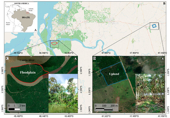
Figure 1.
Study areas in Brazil (A) include: (i) estuarine floodplain area (AV), located in the municipality of Belém (B,C), and (ii) upland area (ATF), located in the municipality of Santa Maria do Pará (B,D).
The studied upland area (ATF) (Figure 1D) is located in Santa Maria do Pará municipality (1°20′10.0′′ S and 47°30′04.0′′ W). The climate is classified as Af according to the Köppen–Geiger classification [35], with an average annual air temperature of 27 °C and annual precipitation of 2250 mm [36]. Consistent with the estuarine floodplain climate pattern, we distinguished between two seasonal precipitation phases: a high-rainfall wet season and a low-rainfall dry season. The soils are classified as Yellow Latosol with a medium sandy texture [37]. In this already degraded area, açaí was planted in 2011 with a spacing of 5 m × 5 m, resulting in a density of 400 clumps per hectare. Each clump can contain up to three stems and is organically fertilized, without the application of soluble chemical fertilizers.
2.1. Experimental Design
2.1.1. Experiment on Upland
The measurements to assess spatial variation in ATF were conducted in September 2020 (dry season), simultaneously at high topography (plateau, Top1), and low topography (lowland, Top2). The two points were spaced approximately 50 m apart, with an elevation difference in less than 2 m (<4%). In each topography zone, four rings were previously fixed (30 min before measuring fluxes) along the açaí planting row (L) and four in the inter-row area (R) where machines operate (Figure 2a). These were placed in a homogeneous açaí plantation area (Figure 2a), located in the municipality of Santa Maria do Pará (Figure 1B,D).
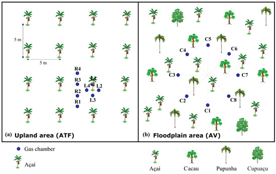
Figure 2.
Experimental design for flux measurements included two distinct configurations: (a) in upland açaí plantation (ATF, Santa Maria do Pará), with eight measurement chambers—four chambers positioned within açaí palm rows (L) surrounding plant clumps, and four chambers in inter-row spaces (R), and (b) in the estuarine floodplain (AV, Belém), with arranged eight chambers (C) in a randomly spatial distribution. Chamber locations are indicated by blue dots.
To assess potential topographic effects on GHG fluxes, we conducted simultaneous measurements across varying elevations (Top1 and Top2). Data collection occurred hourly from 09:00 to 17:00 (local time) from 21 to 25 September 2020. For comparison with the floodplain forest (AV), identical measurement protocols were followed from 14 to 18 September of the same year. The floodplain forest experimental design is detailed in the following section.
2.1.2. Experiment on Floodplain
The experimental design in the VA area was implemented at the highest topographic position (Top A). As previously noted, this site has been modified for optimized açaí production, resulting in reduced native tree density and a structure resembling an agroforestry system. Unlike the ATF area (Figure 2a), the VA’s periodic flooding prevents mechanization, leading to a random spatial distribution of açaí palms through natural regeneration and planting without organized rows. To account for this natural variability, we measured GHG fluxes using eight randomly distributed sampling chambers within a 7 m radius (Figure 2b).
2.1.3. Comparison Between Dry Land and Floodplain
During the rainy season (3–7 April 2021), GHG fluxes were assessed only in Top1 (ATF) and TopA (AV). Measurements were conducted hourly from 08:00 to 17:00 in both locations, following the same methodology previously described (Figure 2). In the ATF, where planting followed a uniform layout, fluxes were measured sequentially at four points along the L and four points in the R (Figure 2a). In AV, the measurement points were randomly allocated in a 700 cm diameter circle (Figure 2b).
2.2. Trace Gas Flux Measurements
The closed dynamic chamber methodology [13] was utilized to measure soil CO2 (FCO2) and CH4 (FCH4) fluxes. The flux chambers were made from polyvinyl chloride (PVC) rings (12.0 cm height × 20.0 cm diameter), that were inserted approximately 4.0 cm deep into the soil (Figure 2). During each measurement period, the rings were sequentially closed with a lid for three minutes, forming the flux chamber. This chamber was connected to a Los Gatos portable gas analyzer (Ultra-portable Greenhouse Gas Analyzer, Warminster, PA, USA), which recorded the gas concentrations (ppm) inside the chamber at two second intervals [38]. Following each measurement session, we determined the volume of each chamber by measuring the height of each ring at four equidistant points using a ruler [13]. The FCO2 and FCH4 values were calculated from the linear rate change in GHG concentrations (ppm s−1) inside the closed dynamic chamber [9,39]. The flux calculation followed the equation: Flux = (dc/dt) × (V/A) × (P/RT), where dc/dt is the concentration slope over time, V is chamber volume (cm3), A is soil surface area (cm2), P is atmospheric pressure (atm), R is the gas constant, and T is air temperature (K) [39]. The flux was considered zero when the linear regression achieved an R2 < 0.30 [40].
2.3. Soil Sampling and Analysis and Environmental Characterization
After each measurement period (ATF and AV), six soil samples were collected using an auger at a depth of 0–10 cm. In the ATF, three samples were collected in the L and three in the R at each flux measurement point (Figure 2). The samples were appropriately conditioned and sent to the Chemical Analysis Laboratory of the Emílio Goeldi Museum, located in Belém (PA).
The concentration of C and N in microbial biomass was investigated using the soil microwave irradiation method [41], conducted only during the dry period due to a lack of chemicals in the laboratory. The determination of microbial biomass carbon (Cm) was performed through Dichromate oxidation [42,43]. The quantification of nitrogen in microbial biomass (Nm) followed the method by [44], substituting fumigation with irradiation. For this, we used the equation proposed by [45], which calculates the difference between the amount of N in irradiated and non-irradiated soil divided by the constant k (k = 0.45). Samples of fine (diameter ≤ 0.2 mm; RF) and coarse (diameter > 0.2 mm; RG) root biomass were collected during both dry and rainy seasons, at a depth of 10 cm, in the previously described ATF and AV locations. After separation from the soil, the roots were oven-dried at 65 °C for 72 h and weighed using an analytical balance [39]. Soil pH was measured using a potentiometer in deionized water, and calibrated with standard solutions of pH 4.0 and pH 7.0 [46]. Soil moisture determination (Us; %) was conducted using the gravimetric method [46].
2.4. Environmental Characterization
Precipitation data for the AV were provided by the National Institute of Meteorology [36], with the automatic data collection station located in Belém (1°26′09.00′′ S and 48°26′14.00′′ W). For the ATF, precipitation data were supplied by the National Water and Basic Sanitation Agency [47], with the meteorological station located in Santa Maria do Pará (1°21′24.5′′ S; 47°34′27.5′′ W). During the trace gas flux measurements, soil temperature (Ts, °C) was quantified using a portable digital thermometer (TP101). Additionally, air temperature (Ta, °C) and relative humidity (HR, %) were recorded every 5 min using a Hobo pro V2 data logger.
2.5. Statistical Analysis
The topographical variation in ATF was compared to that of the estuary’s AV. In the ATF, hourly and daily analyses were conducted using subdivided plots, with two treatments (high and low topography) divided into row (L) and inter-row area (R). The Shapiro–Wilks method was used to assess the normality of the FCH4 and FCO2 data and the soil physicochemical parameters. When normality was not achieved, logarithmic transformations were applied. Student’s t-test was used to determine if there were differences in the means between the times and days of data collection at the same site and between the studied sites. Significant differences (p < 0.05) in flux between the different locations were evaluated using ANOVA and Tukey’s LSD test. Pearson correlation coefficients were calculated to establish the connections between environmental variables and gas fluxes in the months (dry and rainy seasons) when soil chemical characteristics were analyzed simultaneously with gas flux measurements. The free statistical software Infostat 2015® [48] was used to perform the statistical analyses.
3. Results
3.1. Carbon Dioxide and Methane Flux
3.1.1. Spatial Analysis of Homogeneous Açaí Planting in the Dry Season
The results (mean ± standard error) of GHG fluxes in different topographies in the dry season, measured simultaneously, showed unexpected spatial and temporal behavior. The FCO2 was significantly higher (p < 0.01) in Top2 (19.561 ± 0.522 g CO2 m−2 d−1) compared to Top1 (7.416 ± 0.292 g CO2 m−2 d−1). In Top1, there was significant variation (p < 0.01) between the analyzed days. The highest CO₂ effluxes were observed on the fifth day of sampling (15.997 ± 0.229 g CO2 m−2 d−1), followed by the second day (9.827 ± 0.688 g CO2 m−2 d−1), with both being significantly higher (p < 0.01) than the first (6.900 ± 0.229 g CO2 m−2 d−1) and third days (5.057 ± 0.187 g CO2 m−2 d−1). The third day did not differ statistically (p > 0.05) from the fourth day of analysis (4.772 ± 0.215 g CO2 m−2 d−1). In Top2, there was no significant variation (p > 0.05) in FCO2 over the five days of analysis.
Only in the plateau topography (Top1) did FCO2 vary significantly between the analyzed time periods, being higher (p < 0.05) between 09:00 and 12:00 compared to other times (Figure 3A). In Top1, FCO2 levels were higher in the early morning (09:00 to 12:00) compared to other times (Figure 3C), with significantly higher values (p < 0.01) in L (8.187 ± 0.449 g CO2 m−2 d−1) compared to R (6.582 ± 0.362 g CO2 m−2 d−1). However, in Top2 the fluxes did not vary between time periods but were significantly higher (p < 0.001) in L (25.834 ± 0.734 g CO2 m−2 d−1) compared to R (13.017 ± 0.253 g CO2 m−2 d−1) across all time periods (Figure 3E).
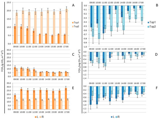
Figure 3.
(A) CO2 flux (FCO2; g CO2 m−2 d−1) in high topography (Top1) and low topography (Top2) in the dry period; (B) CH4 flux (FCH4; mg CH4 m−2 d−1) in Top1 and Top2 in the dry season; (C) FCO2 in Top1 comparing lines (L) with streets (R) in the dry period; (D) FCH4 in Top1 comparing L with R in the dry period; (E) FCO2 in Top2 comparing L with R; (F) FCH4 in Top2 comparing L with R in the dry period in a homogeneous açaí plantation on dry land, located in the municipality of Santa Maria do Pará (Brazil).
On all the analyzed days, there was a consumption of CH4 from the planetary atmosphere (Figure 3). On average, the CH4 influx was significantly higher (p < 0.001) in Top2 (−0.540 ± 0.037 mg CH4 m−2 d−1) compared to Top1 (−0.291 ± 0.038 mg CH4 m−2 d−1). In Top1, the CH4 influx was significantly higher on the fifth day of sampling (−0.835 ± 0.155 mg CH4 m−2 d−1), while no significant differences were observed between the other days (−0.236 ± 0.038 mg CH4 m−2 d−1). In Top2, no significant variation (p > 0.05) in CH4 influx was observed across the analyzed days. The CH4 influx was higher during the morning (until 12:00) compared to the afternoon in Top1 (Figure 3D), with no significant difference (p = 0.221) in fluxes between L (−0.259 ± 0.054 mg CH4 m−2 d−1) and R (−0.383 ± 0.057 mg CH4 m−2 d−1). In Top2, the influx was also higher in the morning compared to the afternoon (Figure 3F), with a significant variation (p < 0.01) in FCH4 between L (−0.683 ± 0.054 mg CH4 m−2 d−1) and R (−0.440 ± 0.052 mg CH4 m−2 d−1).
3.1.2. Simultaneous Flow Measurements in Upland and Floodplains
When comparing simultaneous measurements in ATF and AV, the distribution of GHG fluxes did not follow a normal distribution (p < 0.001) in either location, even after logarithmic transformation. Consequently, a non-parametric test was selected to compare the means. The mean FCO2 in ATF (20.691 ± 0.563 g CO2 m−2 d−1) was higher (H = 101.532; p < 0.001) than in AV (12.869 ± 0.475 g CO2 m−2 d−1). During the rainy season, FCO2 in ATF did not show significant variation (H = 6.906, p = 0.647) across the sampled times. However, in AV, FCO2 levels were significantly lower (H = 45.171, p < 0.001) in the late afternoon, starting from 15:00 (Figure 4A).
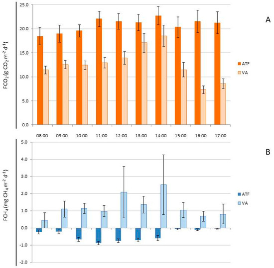
Figure 4.
(A) CO2 flux (FCO2; g CO2 m−2 d−1) in homogeneous açaí plantation (upland, ATF) and a managed floodplain forest (VA) during the rainy season; (B) CH4 flux (FCH4; mg CH4 m−2 d−1) in a homogeneous açaí plantation (upland, ATF) and a managed floodplain area (VA) during the rainy season.
In the rainy season, CH4 uptake was observed in ATF (−0.464 ± 0.038 mg CH4 m−2 d−1), significantly lower (H = 137.451, p < 0.001) than the efflux observed in AV (1.278 ± 0.255 mg CH4 m−2 d−1). In ATF, the CH4 influx was significantly higher (H = 62.835, p < 0.001) between 10:00 and 13:00 compared to the other analyzed time periods (Figure 4B). However, during the same rainy season, in AV, the fluxes did not vary significantly (H = 4.755, p = 0.804) across the analyzed time periods (Figure 4B).
3.2. Seasonal Flux of Greenhouse Gases
When comparing GHG fluxes along the L and R in ATF during the two months of the rainy season on the plateau (Top1-Rainy) and the dry season on both the plateau (Top1-Dry) and lowland (Top2-Dry), a significant difference was observed between the sampled locations (Figure 5A). During both seasons, in Top1 and Top2 (only during the dry season), FCO2 was significantly higher (p < 0.001) in L compared to R (Figure 5). However, regarding FCH4, only in Top2 during the dry season was the CH4 influx significantly higher in L compared to R (Figure 5B), with no significant differences (p > 0.05) in other measurements.
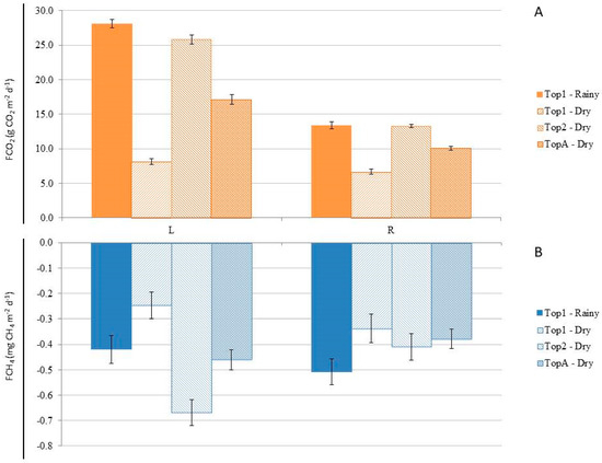
Figure 5.
(A) CO2 efflux (FCO2) in the upland area (ATF) in the plateau (Top1), shoal (Top2), and average (TopA) topography during the months sampled in the wet and dry season. (B) CH4 influx (FCH4) in the upland area (ATF) in the plateau (Top1), shoal (Top2), and average (TopA) topography, during the months sampled in the wet and dry season. The bars represent the standard error of the mean.
In March (rainy season), when fluxes were measured simultaneously, FCO2 was significantly higher (H = 101.532, p < 0.001) in ATF (20.691 ± 0.563 g CO2 m−2 d−1) compared to AV (12.869 ± 0.475 g CO2 m−2 d−1) (Figure 6A). However, in September (dry season), FCO2 was significantly lower (H = 290.921, p < 0.001) in ATF at Top1 (7.416 ± 0.292 g CO2 m−2 d−1) than at Top2 (19.561 ± 0.522 g CO2 m−2 d−1), where the efflux did not differ significantly from FCO2 in AV (20.647 ± 1.741 g CO2 m−2 d−1) (Figure 6C). When considering both topographies in ATF as a single high topography (Top1), the fluxes in AV were significantly higher (H = 15.664, p < 0.001) than in ATF (13.590 ± 0.400 g CO2 m−2 d−1). In ATF, the FCO2 measured during the rainy season was significantly higher (H = 102.696, p < 0.001) than the efflux during the dry season. Conversely, in AV, the CO2 efflux during the dry season was significantly higher (H = 23.636, p < 0.001) than during the rainy season.
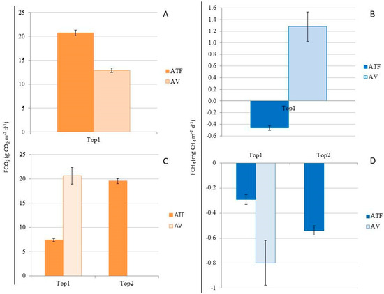
Figure 6.
(A) CO2 flux (FCO2; g CO2 m−2 d−1) in the rainy season (March) in homogeneous açaí plantation in upland (ATF) and in managed floodplain (AV), in high topography (Top1); (B) CH4 flux (FCH4; mg CH4 m−2 d−1) in the rainy season (March) in homogeneous açaí plantation in terra firme (ATF) and in managed várzea forest (AV, in high topography (Top1); (C) CO2 flux (FCO2; g CO2 m−2 d−1) in the dry season (September) in homogeneous açaí plantation in upland (ATF) in high topography (Plateau; Top1) and low topography (Lowlands; Top2), and in managed floodplain (VA), in high topography (Top1); (D) CH4 flux (FCH4; mg CH4 m−2 d−1) in the dry season (September) in homogeneous açaí plantation in upland (ATF) in high topography (Top1) and low topography (Top2), and in managed floodplain (AV) in high topography (Top1).
In March (rainy season), when the flows were measured simultaneously in the two places, the FCH4 was higher (H = 137.451, p < 0.001) in AV (1.278 ± 0.255 mg CH4 m−2 d−1) compared to the influx in ATF (−0.464 ± 0.0375 mg CH4 m−2 d−1) (Figure 6B). However, in September (dry season), the CH4 influx in the high topography (Top1) of AV (−0.798 ± 0.179 mg CH4 m−2 d−1) did not differ from the CH4 influx in the lowland (Top2) of ATF (−0.539 ± 0.037 mg CH4 m−2 d−1), both of which were higher (H = 52.422, p < 0.001) than the CH4 influx on the Top1 (−0.292 ± 0.039 mg CH4 m−2 d−1) (Figure 6D). The average CH4 influx in AV was higher (H = 10.302, p < 0.001) than in ATF (−0.418 ± 0.0273 mg CH4 m−2 d−1) when comparing flux rates across both topographies. In ATF, the CH4 influx measured during the rainy season did not differ (p > 0.05) from that during the dry season. However, in AV, the CH4 efflux during the rainy season was higher (H = 33.407, p < 0.001) than the influx during the dry season.
3.3. Environmental Variables
The total annual precipitation (from August 2020 to July 2021) was 2634.0 mm in the Santa Maria do Pará region (ATF) and 3915.3 mm in the Belém region (AV) (Figure 7A). For both ATF and AV, the wet season spanned from December to May, with climatological totals of 1588.0 mm and 1760.0 mm, accounting for 81.5% and 83.6% of the total annual precipitation, respectively (Figure 7B). The dry season occurred from June to November in both locations, accounting for 18.5% of total rainfall in ATF and 16.4% in AV. Precipitation was consistently lower in ATF compared to AV, except during the months of May, July, and August (Figure 7A). During the study period, rainfall exceeded the climatological averages by 538 mm and 1596 mm in ATF and AV, respectively, coinciding with a La Niña event (Figure 7B). In both locations, precipitation was above the climatological average (values above zero) for most of the months studied, particularly during the dry season (Figure 7B).
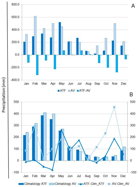
Figure 7.
(A) Precipitation (mm) in the dry land area (ATF) in Santa Maria do Pará, compared to the floodplain area (AV) in Belém, and the difference in precipitation between the two locations (ATF–AV), from 2020 to 2021; (B) Climatology (mm) in the dry land area (Climatology ATF) in Santa Maria do Pará in the floodplain area (Climatology AV) in Belém, and the difference between precipitation (mm) during the study period and the Climatology in ATF (ATF—Clim_ATF) and the Climatology in AV (AV—Clim_AV).
Air temperature and relative humidity (UR) did not follow a normal distribution, necessitating the use of non-parametric tests to compare the means. Temperatures were highest between 12:00 and 14:00 (Figure 8) in both ATF (H = 264.327, p < 0.001) and AV (H = 128.898, p < 0.001). Additionally, temperatures were higher during the dry season compared to the rainy season in both ATF (H = 215.845, p < 0.001) and AV (H = 97.727, p < 0.001). The highest temperatures (H = 405.651, p < 0.001) were recorded in AV during the dry season (30.98 ± 0.10 °C), followed by ATF during the dry season (29.05 ± 0.12 °C). These values were significantly higher than those recorded in ATF (27.92 ± 0.14 °C) and AV (27.38 ± 0.10 °C) during the rainy season, respectively.
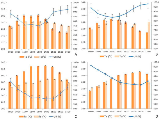
Figure 8.
Behavior of temperature (Ta, °C) and relative humidity (RH, %) of the air, and soil temperature (Ts, °C) in: (A) dry land area (ATF) in the rainy season; (B) floodplain area (AV) in the rainy season; (C) ATF in the dry season; (D) AV in the dry season. Times that have no value were due to the impossibility of collecting the data.
Relative humidity (UR) was higher at 09:00 and 17:00 (Figure 8) in both ATF (H = 175.494, p < 0.001) and AV (H = 157.412, p < 0.001). As expected, UR was higher during the rainy season compared to the dry season in both ATF (H = 368.694, p < 0.001) and AV (H = 124.181, p < 0.001). There was a significant variation when comparing the locations and seasons. During the rainy season, UR was higher in AV (89.59 ± 0.37%) compared to ATF (83.13 ± 0.47%), which did not differ significantly from AV during the dry season (82.65 ± 0.45%). Both of these values were higher than those recorded in ATF during the dry season (67.27 ± 0.38%).
In ATF, soil temperature (Ts) was higher than in AV during both the rainy season (H = 30.10, p < 0.001) and the dry season (H = 16.78, p < 0.001). At both study sites, there was significant variation in Ts across the different sampling times during both the rainy and dry seasons. In ATF, the warmest Ts values were recorded between 11:00 and 15:00 (Figure 8A,C), whereas AV did not show significant variation in Ts throughout the day (Figure 8B,D).
During the rainy season, soil moisture (Us) increased significantly in both ATF (H = 14.29, p < 0.001) and AV (H = 7.50, p < 0.01) compared to dry season values (Table 1). Additionally, Us was consistently higher in the floodplain area (AV) compared to ATF during both the rainy (H = 9.38, p < 0.001) and dry seasons (H = 10.59, p < 0.001). Soil pH did not show statistically significant differences (p > 0.05) between the seasons in either of the sampled areas (Table 1). However, pH was higher in ATF during both the rainy (H = 7.38, p < 0.01) and dry seasons (H = 4.27, p < 0.05) when compared to AV. Fine root biomass did not differ significantly (p > 0.05), either seasonally within each site or between the sites within the same season (Table 1).

Table 1.
Seasonality of some environmental data in upland (ATV) and floodplain (AV) treatments in the eastern Amazon region. Numbers report the mean ± standard error, with lowercase letters comparing the seasonality in each treatment, and uppercase letters comparing treatments in the same seasonality. ND means that there was no analysis.
In ATF, root biomass (RG) was higher during the rainy season (H = 8.20, p < 0.01), whereas in AV, it was higher during the dry season (H = 4.34, p < 0.05). However, when comparing the two sites, RG differed only during the rainy season (Table 1), being higher in ATF (H = 13.95, p < 0.001) compared to AV (Table 1). Microbial carbon (Cmic) and microbial nitrogen (Nmic) were analyzed only during the dry season, with both Cmic and Nmic being higher in AV (HCmic = 8.00, p < 0.01; HNmic = 8.00, p < 0.01) compared to ATF (Table 1).
3.4. Correlations Between Flow and Environmental Variable
In ATF during the rainy season, FCO2 showed positive correlations with Us, RG, TR, and Ta, while exhibiting negative correlations with RF, UR, Pa, and pH (Table 2). Conversely, FCH4 was positively correlated with Us, UR, and Pa, and negatively correlated with Ts and Ta (Table 2). During the dry season, FCO2 showed positive correlations with Us, RF, Cm, and pH, while displaying negative correlations with FCH4, Ts, and RG (Table 2). Meanwhile, FCH4 was positively correlated with Ts, RG, and Nm, and negatively correlated with Us, RF, Pa, Cm, and pH (Table 2).
Table 2.
Correlation coefficient between CO2 (FCO2) and CH4 (FCH4) fluxes with soil temperature (Ts), soil moisture (Us), fine root biomass (RF), coarse root biomass (RG), total root biomass (TR), air temperature (Ta), relative humidity (UR), atmospheric pressure (Pa), microbial carbon (Cm), microbial nitrogen (Nm), pH in açaí monoculture grown on dry land (ATF), and açaí agroforestry in the estuary floodplain area (AV) in the rainy and dry seasons.
In AV during the rainy season, FCO2 was positively correlated with FCH4, Ts, RF, RG, TR, and Ta, while showing negative correlations with Us, UR, Pa, and pH (Table 2). In the same season, FCH4 did not show significant correlations with any of the analyzed variables, except for a positive correlation with FCO2. During the dry season, only FCO2 exhibited positive correlations with Ta and UR (Table 2).
4. Discussion
4.1. Soil Carbon Flux in Açaí Plantation on Dry Land
During the dry season, in a La Niña year when rainfall significantly exceeded the climatological average (Figure 7B), the soil FCO2 on the plateau (Top1) in ATF was considerably lower than the efflux in the lowland (Top2) area (Figure 6B). These results differ markedly from those conducted in pristine Guianas tropical forest where no variation in CO2 fluxes was found across different topographies, including plateaus and lowlands areas [23]. An important consideration is that in our study fluxes were measured simultaneously in both topographies using laboratory-calibrated equipment, with no statistical variation between the instruments. The necessity of simultaneous sampling emerges from the coupled influences of atmospheric dynamics and pedohydrological conditions on flux magnitudes and directions.
We observed that the hourly variation of FCO2 was significant only in the plateau area compared to the lowland, with higher fluxes in the morning compared to the other times. This indicates that CO2 flux measurements performed on the plateau, at a specific time of day, can result in a significant error in this environment. However, in relation to FCH4, the error may be even greater, since in both topographies the fluxes were higher in the morning compared to the afternoon. Our results demonstrate consistent diurnal variability in CO2 and CH4 fluxes across both dry and wet seasons—a phenomenon that remains understudied in tropical ecosystems. Few studies to date have explicitly addressed these hourly scale dynamics, highlighting a critical gap in understanding temporal flux patterns in such environments.
To explain the difference in CO2 efflux, fine root (RF) biomass was significantly higher (LSD = 0.814; p < 0.01) in Top2 (3.762 ± 0.222 Mg ha−1) compared to Top1 (2.212 ± 0.309 Mg ha−1). Similarly, soil moisture (Us) was higher (LSD = 2.425; p < 0.05) in Top2 (11.085 ± 1.036%) than in Top1 (8.641 ± 0.508%). Additionally, microbial biomass was greater (LSD = 0.106; p < 0.001) in Top2 (0.537 ± 0.047 kg Cmic kg−1 soil) compared to Top1 (0.293 ± 0.021 kg Cmic kg−1 soil). In this context, the lowland area exhibited 22.0% higher moisture than the plateau area, directly influencing nutrient and organic matter dynamics. This increase promoted greater fine root biomass [23] and microbial biomass [48], which in turn resulted in significantly higher CO2 efflux. This may explain the greater soil respiration observed in the lowland area of an organic açaí plantation on upland terrain. Thus, soil organic matter plays a crucial role in maintaining water and microbial activity, enhancing ecosystem productivity in homogeneous açaí plantations [49].
When comparing the lines (L) and streets (R), the FCO2 during the dry season in Top1 was 8.154 ± 0.450 g CO2 m−2 d−1 in L, which was significantly lower (H = 172.510; p < 0.001) than the 25.825 ± 0.667 g CO2 m−2 d−1 in L in Top2. In R, the FCO2 in ATV in Top1 was 6.672 ± 0.361 g CO2 m−2 d−1, which was also significantly lower (H = 117.794; p < 0.001) than the 13.297 ± 0.263 g CO2 m−2 d−1 in Top2. When comparing the rainy season to the dry season, only in Top1 were both FCO2 in L and R significantly higher (p < 0.001) during the rainy season compared to the dry season (Figure 3A). The results reveal that, in both L and R, the lowland topography (Top2) emits more CO2 into the atmosphere compared to the plateau (Top1), a finding that contrasts with observations in an Acacia mangium plantation in Indonesia [50] and in a primary upland forest in the Amazon [51]. On the other hand, studies conducted in a closed-canopy upland forest in the central Amazon [52] and in a mangrove forest in the Amazon estuary [39] identified significant topographic variation, although, unlike the results presented here, the fluxes were higher in elevated topography compared to lowland areas. While A. mangium trees and E. oleracea palms differ substantially in physiology, their gas flux spatial patterns remain comparable. Interestingly, the Indonesian study reported higher emissions from plateau areas than lowlands—a pattern contrasting sharply with our ATF observations. Our findings suggest that the higher CO₂ efflux in low-lying areas can be attributed to their 22.0% greater soil moisture compared to the plateau, as previously discussed.
The annual average FCO2 efflux was higher (H = 166.519; p < 0.001 in L (21.025 ± 0.543 g CO2 m−2 d−1) than in R (11.251 ± 0.275 g CO2 m−2 d−1), which could not be explained by root biomass (fine, coarse, or total), as no statistical variation (p > 0.05) was observed between L and R. However, the data show that soil moisture (Us) was significantly higher (H = 5.859; p < 0.05) in L (28.458 ± 3.434%) compared to R (18.423 ± 3.262%). During the dry season, irrigation is applied only to the açaí planting rows (L), which may enhance soil biological activity in upland areas of the Amazon region.
In the upland açaí plantation, the FCO2 in the plateau (Top1) topography was significantly higher (H = 253.615, p < 0.001) during the rainy season (20.691 ± 0.563 g CO2 m−2 d−1) compared to the dry season (7.388 ± 0.292 g CO2 m−2 d−1). Despite daily irrigation during the dry season and the occurrence of a La Niña year, CO2 fluxes remained higher during the rainy season in both when comparing the L and the R. Root biomass did not differ (p > 0.05) between the seasons; however, soil moisture (Us) mirrored the differences in FCO2, being significantly higher (H = 19.355, p < 0.001) during the rainy season (23.118 ± 0.765%) compared to the dry season (8.641 ± 0.508%). On the other hand, soil temperature (Ts), although showing only a slight difference, was significantly higher (H = 30.171, p < 0.001) during the dry season (27.989 ± 0.071 °C) compared to the rainy season (27.371 ± 0.075 °C). Multiple studies across tropical forests ecosystems have consistently demonstrated marked seasonal variability in CO2 efflux, with higher emission rates observed during the rainy season compared to the dry periods [50,53,54,55], a pattern also observed in an agroforestry system in Panama [56]. The data suggest that, despite irrigation during the dry season, it may not be sufficient to maintain soil productivity in upland açaí plantations.
We concur with the assertion that soil respiration serves as a reliable proxy for belowground carbon allocation, with higher CO2 fluxes typically indicating greater soil productivity. While our findings are based on measurements conducted over five-day periods during both dry and wet seasons, they reveal noteworthy patterns in açaí plantation ecosystems. Specifically, the observed annual flux of 5.9 kg CO₂ m−2 yr−1 was approximately six-fold and three-fold higher than values reported for degraded pasture and secondary forest in Paragominas, respectively [55]. This disparity becomes particularly striking when compared to data from the Tapajós rainforest, where root biomass of 292 g m−2 yielded 1.9 kg CO₂ m−2 y−1 [57],which are nearly identical to our measured root biomass (299 g m−2) but producing only one-third of the CO₂ efflux. These comparisons suggest that managed açaí plantations, potentially due to irrigation practices, may exhibit substantially enhanced belowground productivity (microbial activity and root respiration) compared to both natural and degraded ecosystems.
During the dry season, the influx of CH4 from the atmosphere into the soil of the açaí plantation was significantly higher (H = 42.392, p < 0.001) in Top2 (−0.539 ± 0.034 mg CH4 m−2 d−1) compared to Top1 (−0.332 ± 0.024 mg CH4 m−2 d−1). Only in Top2 was the CH4 influx significantly higher (H = 8.134, p < 0.01) in the lines (L) (−0.670 ± 0.051 mg CH4 m−2 d−1) compared to the streets (R) (−0.409 ± 0.052 mg CH4 m−2 d−1) during the dry season. These results differ from those observed in an A. mangium plantation in Indonesia [50], where the CH4 influx from the atmosphere was higher in the plateau compared to the lowland. As previously mentioned, both soil moisture (Us) and microbial biomass were higher in Top2, explaining the greater microbial activity and, consequently, the higher CH4 influx from the planetary atmosphere. We understand that the higher Us in the lowland (11.085 ± 1.036%) was not sufficient to negatively influence the permeability of CH4 and atmospheric O2 into the soil [13,58], allowing the influx of CH4 from the atmosphere to be consumed in the soil.
Only in Top2 was the influx of atmospheric CH4 significantly higher (H = 8.134, p < 0.01) in the L (−0.670 ± 0.051 mg CH4 m−2 d−1) compared to the R (−0.409 ± 0.052 mg CH4 m−2 d−1). As previously shown, in this same topography, soil moisture (Us) was higher in L compared to R, indicating that methanotrophic activity was not hindered at Us levels close to 29%. In fact, the higher Us in the planting lines enhanced the activity of these organisms compared to the streets, and the diffusion of CH4 and atmospheric O2 into the soil was not impaired. When comparing only Top1, seasonality did not influence the influx of atmospheric CH4 (p > 0.05), with values of −0.360 ± 0.031 mg CH4 m−2 d−1 during the rainy season and −0.291 ± 0.038 mg CH4 m−2 d−1 during the dry season.
Methane possesses a global warming potential 32 times greater than CO2 over a 100-year timescale [59]. In this context, the removal of 1 Mg (Mega gram) of CH4 has a significant impact on global warming [60]. Additionally, with an average tropospheric lifetime of about 10 years [61], land-use practices that reduce CH4 emissions or contribute to the capture of atmospheric CH4 can play a major role in global climate change mitigation. In this regard, organic açaí plantations in upland areas are estimated to absorb an average of 1.6 ± 0.080 kg CH4 ha−1 yr−1, which is slightly lower than the values predicted in previous studies for different ecosystems, particularly when compared to the 2.7 kg CH4 ha−1 yr−1 for tropical soils [62] and significantly lower than the 2.5–4.0 kg CH4 ha−1 yr−1 removed by a secondary forest enriched with leguminous trees [54]. However, the observed atmospheric CH4 uptake rate closely both the 1.0 kg CH4 ha−1 yr−1 reported for a secondary forest in the eastern Amazon [13] and the 1.6 ± 0.9 kg CH4 ha−1 yr−1 removed by the soil in Tapajós National Forest [63]. Most importantly, land use with organic and homogeneous açaí plantations in upland areas does not produce methane, even with the use of irrigation.
4.2. Soil Carbon Flux During the Rainy Season in Upland Planting Compared to Estuary Floodplain
It is important to note that during the rainy season, measurements in ATF and AV were conducted simultaneously using two laboratory-calibrated devices with no statistical variation between them. The FCO2 in ATF (16.176 ± 0.347 g CO2 m−2 d−1) was significantly higher (H = 19.286, p < 0.001) than the flux in AV (12.813 ± 0.477 g CO2 m−2 d−1). On the sampling days and at all sampled times, the FCO2 was higher in ATF compared to the efflux in AV (Figure 4A). Studies comparing CO2 efflux between upland and floodplain ecosystems are scarce in the literature, especially those that measure simultaneously in both locations. Therefore, our comparison can only be made across distinct sites, though efforts were made to maintain similar ecosystem variations. Two-year measurements conducted in the Caxiuanã National Forest showed that the flux on the plateau (sandy soil) was 21.0% higher than in the lowland (clay soil) [51]. A study conducted in a region with significant topographic variation (25 m between plateau and lowland) in China, found that the plateau area produced 11.9% more CO2 [64]. Similarly, in a topographic variation study in Guyana, the FCO2 was 11.7% higher on the plateau compared to the lowland [23]. Consistent with these studies, our results during the rainy season show a 20.8% higher CO2 production in upland area (sandy soil—plateau) compared to floodplain area of the Amazon estuary (clay soil—lowland).
Some studies suggest that the difference in soil FCO2 between plateau and lowland is related to higher root biomass in sandy soils compared to clay soils [65]. In the present study, the higher CO2 efflux in ATF during the rainy season can be explained by root biomass, as the total live root biomass in ATF (11.839 ± 1.041 Mg ha−1) was twice as high (p < 0.001) compared to AV (5.643 ± 0.891 Mg ha−1). During the rainy season, FCO2 showed a significant negative correlation with fine root (RF) and positive correlations with both coarse root (RG) and total root biomass (TR) (Table 2). Unfortunately, we were unable to measure microbial carbon and nitrogen during this period, which would have allowed for a more detailed discussion of these results. Nevertheless, the entry of water into the soil, whether through rainfall, irrigation, or tidal movement, is associated with the immediate replacement of air-filled pores with water. This influx of water can initially expel air from the soil pores and subsequently form an insulating layer, hindering the diffusion of CO2 from the soil to the atmosphere [66], thereby reducing soil respiration [67]. Consistent with these findings, rainy season FCO2 in ATF showed positive correlations with soil moisture (Us) and soil temperature (Ts), but negative correlations with relative humidity (UR) and atmospheric pressure (Pa) (Table 2). Other studies have also indicated correlations between FCO2 and temperature [68,69] as well as soil moisture [70].
During the same rainy season, the CH4 efflux in AV (1.033 mg CH4 m−2 d−1) was significantly higher (H = 122.733; p < 0.001) than the CH4 influx in ATF (−0.360 mg CH4 m−2 d−1). On all analyzed days, a high production of CH4 was observed in AV, while an influx of CH4 was recorded in ATF (Figure 4B). The production/influx of CH4 are microbiological processes primarily regulated by the absence/presence of oxygen, respectively, and the presence of labile organic substrates [71]. Consequently, the higher soil moisture (Us) in AV (Table 1) facilitates the proliferation of methanogenic processes (microbial production of CH4). In contrast, aerobic soils in ATF promote methanotrophy (microbial consumption of CH4). This explains the negative correlation with soil temperature (Ts) and the positive correlation with soil moisture (Us) (Table 2), as Ts negatively affects the physiology and proliferation of microorganisms, while Us positively influences root growth, respiration, and microbial activity. In upland areas (ATF) with homogeneous organic açaí plantations, 34.9% of the CH4 produced in managed floodplain areas for açaí production in the estuary is removed daily. The lack of comparative studies between upland forest production systems and floodplain environments hinders meaningful interpretation of our results.
Soils in tropical upland areas are generally considered sinks for atmospheric CH4, and changes in land use, such as the homogeneous planting of açaí in this case, can reduce the intensity of this sink [72]. Such land-use changes can additionally deplete soil organic carbon stocks, thereby compromising the ecosystem’s overall carbon sequestration potential [73]. The influx of atmospheric CH4 in the organic açaí plantation in upland areas during the rainy season was 1.7 ± 0.1 kg CH4 ha−1 yr−1, while the production of CH4 in the estuarine floodplain during the same period was 4.6 ± 0.9 kg CH4 ha−1 yr−1. Concurrent measurements during the rainy season revealed that CH4 production in AV was 2.7 times higher compared to the uptake in ATF (Figure 5B). Studies in the state of Rondônia (Brazil) showed that during the rainy season, pasture soils produced 6.1 kg CH4-C m−2 yr−1, whereas soils in primary forest areas consumed 1.1 kg CH4-C m−2 yr−1 [74]. It is understood that in the Amazon, soils with less than 35–40% of pore space filled with water act as CH4 sinks, while those above these values act as sources [75]. In ATF, the soil had an average water content of 23.1%, while in AV it was 53.3%, which appears to align with this premise. The results presented here fall within the range of consumption reported for fine-textured soils in the Amazon rainforest, which was 1.5–2.0 kg CH4 ha−1 yr−1 [13]. Considering that CH4 has a global warming potential 32 times greater than CO2 over a 100-year period [59], the production of CO2-equivalents (CO2-eq) in ATF was 59.1 Mg CO2-eq ha−1 yr−1, while in AV it was 49.3 Mg CO2-eq ha−1 yr−1.
4.3. Annual Soil Carbon Flux in Upland Planting Compared to Estuary Floodplain
FCO2 was positively correlated with FCH4 in AV during the rainy season and negatively correlated with ATF during the dry season (Table 2). In ATF, the sandy soil facilitates air exchange with the atmosphere, enhancing soil respiration and methane oxidation by methanotrophic organisms [76]. This process is hindered in AV due to the highly clayey soil and elevated moisture levels [13,75], as well as the anoxia caused by tidal water movement, which creates conditions favorable for the proliferation of methanogenic bacteria [77].
The increase in CO2 efflux between the rainy and dry seasons (Figure 5A) is likely due to an increase in labile carbon available to microorganisms, greater soil oxygenation, resulting in intense microbial activity, and subsequent degradation of soil organic matter [78,79], which intensifies soil respiration. The onset of the rainy season leads to lower CO2 efflux, which may be necessary to increase soil carbon and recover the carbon lost through decomposition during the dry season [80], when the soil is more aerated. A study in Indonesian forests found drained areas (lower soil moisture and pH) increased CO₂ fluxes, while undrained areas (higher water tables) enhanced CH4 fluxes, confirming methanogenesis under anaerobic conditions [81].
The efflux/influx of CH4 in ATF during the rainy season (Figure 5B) was positively correlated with soil moisture (Us), relative humidity (UR), and atmospheric pressure (Pa), while negatively correlated with soil temperature (Ts) (Table 2). In contrast, during the dry season in ATF, FCH4 was positively correlated with Ts, coarse roots (RG), total roots (TR), and microbial nitrogen (Nm), and negatively correlated with Us, fine roots (RF), Pa, microbial carbon (Cm), and pH (Table 2). In AV, no significant correlations were found between FCH4 and the studied variables during either season (Table 2). Our findings demonstrate that natural precipitation during wet seasons enhances soil moisture, stimulating CH4 production. In contrast, irrigation-induced moisture increases during the dry season appear to suppress methanogenic activity. Other studies have similarly demonstrated a correlation between CH4 flux and soil moisture [19,82], highlighting that soil moisture regulates CH4 uptake by controlling the diffusion of methane and oxygen within the soil atmosphere. Thus, we can confirm that waterlogged conditions promote the activity of methanogenic bacteria due to anoxia. However, as soil moisture decreases, reduced moisture levels favor the proliferation of methanotrophic bacteria, enhancing the diffusion and consumption of atmospheric CH4 [83,84]. This shift in soil moisture may explain the high rates of CH4 consumption observed in AV (Figure 6D). These results demonstrate that high floodplain areas are not always sources of CH4 emissions to the atmosphere; under certain conditions, they can also function as significant sinks for this gas.
A significant positive correlation between variations in soil respiration and soil moisture indicates that, within a certain range, soil moisture is directly proportional to soil respiration. However, excessive increases in soil moisture can create anoxic conditions, hinder gas exchange, reduce respiration, and shift soil from CH4 inflow to efflux. In this sense, the main environmental factors controlling CH4 exchange between soil and the atmosphere are the proportion of pore space occupied by water, the availability and quality of carbon, and soil temperature [58,85,86]. Additionally, root exudates can increase CH4 production in the soil due to the heightened demand for O2 by decomposer organisms, thereby reducing methanotrophy from soil-derived carbon and stimulating intense, short-term changes in soil organic matter recycling (priming effect) [87]. This may explain the strong positive correlation between coarse roots (RG) and total roots (TR) with CH4 flux during the dry season.
The high sensitivity of CH4 dynamics to environmental variables (e.g., soil moisture, microbial diversity, temperature, and atmospheric pressure) makes characterizing both spatial and temporal variability in methane emissions particularly challenging. We agree that a limited number of CH4 flux observations in restored tropical agriculture lands, combined with complex environmental variables governing soil-atmosphere exchange, constrain accurate parameterization of biogeochemical models [88]. This limitation is particularly significant given the complex interplay of factors influencing methane production, oxidation, and transport, such as soil moisture, temperature, organic matter availability, and microbial community dynamics. Estimates of CH4 fluxes from models remain uncertain due to three key limitations: scarce or inadequate field measurements, poorly constrained model parameterizations, and unreliable wetland inventories [89]. As a result, models often rely on simplified representations of these processes, which can lead to uncertainties in predicting CH4 emissions under varying environmental conditions. Our study contributes to filling the knowledge gap on GHG fluxes by comparing restored upland areas using a characteristic floodplain species with the native habitat of this species.
Enhancing model precision requires urgent development of higher-resolution datasets that fully characterize the spatiotemporal dynamics of CH4 fluxes across different ecosystems. Additionally, integrating multi-disciplinary approaches, such as combining remote sensing, eddy covariance measurements, and laboratory experiments, could enhance our understanding of the underlying mechanisms driving methane dynamics. Advances in machine learning and data assimilation techniques also offer promising avenues for refining model parameterizations and reducing uncertainties. Ultimately, a more robust representation of CH4 fluxes in biogeochemical models is crucial for accurately projecting future methane emissions and informing climate change mitigation strategies.
5. Conclusions
Although we conducted intensive sampling (hourly measurements during daylight hours over five consecutive days per sampling period), the lack of monthly measurements represents a limitation of this study. Nevertheless, the upland area produced a total of 59.1 Mg CO2-eq ha−1 year−1, while the floodplain area produced 49.3 Mg CO2-eq ha−1 year−1. During the dry season, spatial heterogeneity in the greenhouse gases flux was identified, with soil CO2 flux and CH4 consumption being higher in the lowland compared to the plateau, across all hours and days analyzed. In the rainy season, simultaneous measurements revealed that the CO2 flux is higher in the upland, while CH4 flux was greater in the floodplain, with atmospheric CH4 consumption on the upland. In the floodplain, CH4 production was observed in the rainy month and consumption in the dry month. In the upland açaí plantation area, CO2 fluxes were higher in the planting row compared to the streets, in both seasons of the year, with no variation in the atmospheric CH4 consumption. Soil moisture and temperature appear to control gas fluxes only in the upland, but in contrasting ways during the two seasons analyzed. Soil organic matter plays a vital role in preserving water and microorganisms, enhancing ecosystem productivity in uniform açaí plantations and intensifying the transfer of CH4 from the atmosphere to the soil. However, excessive soil moisture can create anoxic conditions, block gas diffusion, reduce soil respiration, and potentially turn the soil from a sink into a source of CH4. Our findings demonstrate that rehabilitating degraded areas through açaí cultivation enhances soil productivity while sustaining atmospheric CH4 removal. More detailed studies are needed to understand how greenhouse gas fluxes vary across different topographies in upland areas of the Amazon under agricultural production systems.
Author Contributions
Conceptualization, M.F.A. and J.H.C.; methodology, M.F.A., C.J.R.d.C. and J.H.C.; software, M.F.A. and J.H.C.; validation, M.F.A., C.J.R.d.C. and J.H.C.; formal analysis, M.F.A.; investigation, M.F.A. and J.H.C.; resources, M.F.A., C.J.R.d.C. and J.H.C.; data curation, M.F.A.; writing—original draft preparation, J.H.C.; writing—review and editing, J.H.C.; visualization, M.F.A. and J.H.C. All authors have read and agreed to the published version of the manuscript.
Funding
This research received no external funding.
Data Availability Statement
Data are contained within the article.
Acknowledgments
We would like to thank the residents of Ilha do Combú, especially Odinaldo Pena Quaresma (Didito) and his wife Dóris Lucia Santos Mattos da Cunha for their support in the fieldwork. We would like to thank the Museu Paraense Emilio Goeldi (MPEG), especially the Coordination of Earth Sciences and Ecology, for providing the chemical analysis laboratory, materials and equipment, in addition to the technical assistance from José Paulo Sarmento. We are grateful to the Coordination for the Improvement of Higher Education Personnel (CAPES) for the financial support during the development of the doctoral thesis.
Conflicts of Interest
The authors declare no conflicts of interest.
References
- IPCC. Climate Change 2014: Synthesis Report. Contribution of Working Groups I, II and III to the Fifth Assessment Report of the Intergovernmental Panel on Climate Change; Core Writing Team, Pachauri, R.K., Meyer, L.A., Eds.; IPCC: Geneva, Switzerland, 2014. Available online: https://www.ipcc.ch/report/ar5/syr/ (accessed on 30 June 2024).
- IPCC. Global Warming of 1.5 °C: An IPCC Special Report on the Impacts of Global Warming of 1.5 °C Above Preindustrial Levels and Related Global Greenhouse Gas Emission Pathways: The Context of Strengthening the Global Response to the Threat of Climate Change, Sustainable Development, and Efforts to Eradicate Poverty; IPCC: Geneva, Switzerland, 2018; p. 570.
- Verchot, L.V.; Dannenmann, M.; Kengdo, S.K.; Njine-Bememba, C.B.; Rufino, M.C.; Sonwa, D.J.; Tejedor, J. Land-Use Change and Biogeochemical Controls of Soil CO2, N2O and CH4 Fluxes in Cameroonian Forest Landscapes. J. Integr. Environ. Sci. 2020, 17, 45–67. [Google Scholar] [CrossRef]
- Adachi, M.; Ito, A.; Yonemura, S.; Takeuchi, W. Estimation of Global Soil Respiration by Accounting for Land-Use Changes Derived from Remote Sensing Data. J. Environ. Manag. 2017, 200, 97–104. [Google Scholar] [CrossRef] [PubMed]
- Bossio, D.A.; Cook-Patton, S.C.; Ellis, P.W.; Fargione, J.; Sanderman, J.; Smith, P.; Wood, S.; Zomer, R.J.; von Unger, M.; Emmer, I.M.; et al. The Role of Soil Carbon in Natural Climate Solutions. Nat. Sustain. 2020, 3, 391–398. [Google Scholar] [CrossRef]
- Naidu, D.G.T.; Bagchi, S. Greening of the Earth Does Not Compensate for Rising Soil Heterotrophic Respiration under Climate Change. Glob. Change Biol. 2021, 27, 2029–2038. [Google Scholar] [CrossRef]
- Scheper, A.C.; Verweij, P.A.; van Kuijk, M. Post-Fire Forest Restoration in the Humid Tropics: A Synthesis of Available Strategies and Knowledge Gaps for Effective Restoration. Sci. Total Environ. 2021, 771, 144647. [Google Scholar] [CrossRef] [PubMed]
- Hassler, E.; Corre, M.D.; Tjoa, A.; Damris, M.; Utami, S.R.; Veldkamp, E. Soil Fertility Controls Soil–Atmosphere Carbon Dioxide and Methane Fluxes in a Tropical Landscape Converted from Lowland Forest to Rubber and Oil Palm Plantations. Biogeosciences 2015, 12, 5831–5852. [Google Scholar] [CrossRef]
- Peterson, M.L. Educational Programs for Team Delivery. Interdisciplinary Education of Health Associates. Acad. Med. 1975, 50, 111–117. [Google Scholar] [CrossRef]
- Arunrat, N.; Sansupa, C.; Sereenonchai, S.; Hatano, R.; Lal, R. Fire-Induced Changes in Soil Properties and Bacterial Communities in Rotational Shifting Cultivation Fields in Northern Thailand. Biology 2024, 13, 383. [Google Scholar] [CrossRef]
- Alves, N.d.O.; Brito, J.; Caumo, S.; Arana, A.; Hacon, S.d.S.; Artaxo, P.; Hillamo, R.; Teinilä, K.; Medeiros, S.R.B.d.; Vasconcellos, P.d.C. Biomass Burning in the Amazon Region: Aerosol Source Apportionment and Associated Health Risk Assessment. Atmos. Environ. 2015, 120, 277–285. [Google Scholar] [CrossRef]
- Denardin, L.G.d.O.; Alves, L.A.; Ortigara, C.; Winck, B.; Coblinski, J.A.; Schmidt, M.R.; Carlos, F.S.; Toni, C.A.G.d.; Camargo, F.A.d.O.; Anghinoni, I.; et al. How Different Soil Moisture Levels Affect the Microbial Activity. Ciência Rural 2020, 50, 1–10. [Google Scholar] [CrossRef]
- Verchot, L.V.; Davidson, E.A.; Cattânio, J.H.; Ackerman, I.L. Land-Use Change and Biogeochemical Controls of Methane Fluxes in Soils of Eastern Amazonia. Ecosystems 2000, 3, 41–56. [Google Scholar] [CrossRef]
- Lira-Guedes, A.C.; Leal, G.D.A.; Fischer, G.R.; Aguiar, L.J.G.; Melém, N.J.; Baia, A.L.P.; Guedes, M.C.; Júnior, N.J.; Baia, A.L.P.; Guedes, M.C. Carbon Emissions in Hydromorphic Soils from an Estuarine Floodplain Forest in the Amazon River. Rev. Bras. Ciências Ambient. 2021, 56, 413–423. [Google Scholar] [CrossRef]
- Cattanio, J.H.; Anderson, A.B.; Carvalho, M.S. Floristic Composition and Topographic Variation in a Tidal Floodplain Forest in the Amazon Estuary. Rev. Bras. Botânica 2002, 25, 419–430. [Google Scholar] [CrossRef]
- Salo, M.; Sirén, A.; Kalliola, R.; Wild, D.; Harvest, S. Açaí: The Forest Farms of the Amazon Estuary. In Diagnosing Wild Species Harvest; Salo, M., Sirén, A., Kalliola, R., Eds.; Elsevier: Amsterdam, The Netherlands, 2013; pp. 191–202. ISBN 9780123972040. [Google Scholar]
- Cattânio, J.H.; Davidson, E.A.; Nepstad, D.C.; Verchot, L.V.; Ackerman, I.L. Unexpected Results of a Pilot Throughfall Exclusion Experiment on Soil Emissions of CO2, CH4, N2O, and NO in Eastern Amazonia. Biol. Fertil. Soils 2002, 36, 102–108. [Google Scholar] [CrossRef]
- Davidson, E.A.; Ishida, F.Y.; Nepstad, D.C. Effects of an Experimental Drought on Soil Emissions of Carbon Dioxide, Methane, Nitrous Oxide, and Nitric Oxide in a Moist Tropical Forest. Glob. Change Biol. 2004, 10, 718–730. [Google Scholar] [CrossRef]
- Werner, C.; Zheng, X.; Tang, J.; Xie, B.; Liu, C.; Kiese, R.; Butterbach-Bahl, K. N2O, CH4 and CO2 Emissions from Seasonal Tropical Rainforests and a Rubber Plantation in Southwest China. Plant Soil 2006, 289, 335–353. [Google Scholar] [CrossRef]
- Mosier, A.; Wassmann, R.; Verchot, L.; King, J.; Palm, C. Methane and Nitrogen Oxide Fluxes in Tropical Agricultural Soils: Sources, Sinks and Mechanisms. Environ. Dev. Sustain. 2004, 6, 11–49. [Google Scholar] [CrossRef]
- Carvalho, W.D.; Mustin, K.; Hilário, R.R.; Vasconcelos, I.M.; Eilers, V.; Fearnside, P.M. Deforestation Control in the Brazilian Amazon: A Conservation Struggle Being Lost as Agreements and Regulations Are Subverted and Bypassed. Perspect. Ecol. Conserv. 2019, 17, 122–130. [Google Scholar] [CrossRef]
- Serrano-Silva, N.; Sarria-Guzmán, Y.; Dendooven, L.; Luna-Guido, M. Methanogenesis and Methanotrophy in Soil: A Review. Pedosphere 2014, 24, 291–307. [Google Scholar] [CrossRef]
- Courtois, E.A.; Stahl, C.; Van den Berge, J.; Bréchet, L.; Van Langenhove, L.; Richter, A.; Urbina, I.; Soong, J.L.; Peñuelas, J.; Janssens, I.A. Spatial Variation of Soil CO2, CH4 and N2O Fluxes Across Topographical Positions in Tropical Forests of the Guiana Shield. Ecosystems 2018, 21, 1445–1458. [Google Scholar] [CrossRef]
- Rachor, I.; Gebert, J.; Gröngröft, A.; Pfeiffer, E.M. Assessment of the Methane Oxidation Capacity of Compacted Soils Intended for Use as Landfill Cover Materials. Waste Manag. 2011, 31, 833–842. [Google Scholar] [CrossRef] [PubMed]
- Bodelier, P.L.E.; Roslev, P.; Henckel, T.; Frenzel, P. Stimulation by Ammonium-Based Fertilizers of Methane Oxidation in Soil around Rice Roots. Nature 2000, 403, 421–424. [Google Scholar] [CrossRef] [PubMed]
- Bodelier, P.L.E.; Steenbergh, A.K. Interactions between Methane and the Nitrogen Cycle in Light of Climate Change. Curr. Opin. Environ. Sustain. 2014, 9–10, 26–36. [Google Scholar] [CrossRef]
- Ho, A.; Angel, R.; Veraart, A.J.; Daebeler, A.; Jia, Z.; Kim, S.Y.; Kerckhof, F.M.; Boon, N.; Bodelier, P.L.E. Biotic Interactions in Microbial Communities as Modulators of Biogeochemical Processes: Methanotrophy as a Model System. Front. Microbiol. 2016, 7, 1–11. [Google Scholar] [CrossRef]
- Murase, J.; Frenzel, P. Selective Grazing of Methanotrophs by Protozoa in a Rice Field Soil. FEMS Microbiol. Ecol. 2008, 65, 408–414. [Google Scholar] [CrossRef] [PubMed]
- Campbell, A.J.; Carvalheiro, L.G.; Maués, M.M.; Jaffé, R.; Giannini, T.C.; Freitas, M.A.B.; Coelho, B.W.T.; Menezes, C. Anthropogenic Disturbance of Tropical Forests Threatens Pollination Services to Açaí Palm in the Amazon River Delta. J. Appl. Ecol. 2018, 55, 1725–1736. [Google Scholar] [CrossRef]
- Freitas, M.A.B.; Vieira, I.C.G.; Albernaz, A.L.K.M.; Magalhães, J.L.L.; Lees, A.C. Floristic Impoverishment of Amazonian Floodplain Forests Managed for Açaí Fruit Production. For. Ecol. Manag. 2015, 351, 20–27. [Google Scholar] [CrossRef]
- Brondizio, E.S.; Moran, E.F. Human Dimensions of Climate Change: The Vulnerability of Small Farmers in the Amazon. Philos. Trans. R. Soc. B Biol. Sci. 2008, 363, 1803–1809. [Google Scholar] [CrossRef]
- Dos Santos, J.C.; Sena, A.L.d.S.; Homma, A.K.O. Viabilidade Econômica Do Manejo de Açaizais No Estuário Amazônico: Estudo de Caso Na Região Do Rio Tauerá-Açu, Abaetetuba—Estado Do Pará. In Proceedings of the Sociedade Brasileira de Economia, Administração e Sociologia Rural, Vitória, Brazil, 21 May 2024; pp. 22–25. [Google Scholar]
- Farias Neto, J.T.; Resende, M.D.V.; Oliveira, M.d.S.P. Seleção Simultânea Em Progênies de Açaizeiro Irrigado Para Produção e Peso Do Fruto. Rev. Bras. Frutic. 2011, 33, 532–539. [Google Scholar] [CrossRef]
- Tavares, G.d.S.; Homma, A.K.O.; Menezes, A.J.E.A.d.; Palheta, M.P. Análise Da Produção e Comercialização de Açaí No Estado Do Pará, Brasil. Int. J. Dev. Res. 2020, 10, 35215–35221. [Google Scholar]
- Peel, M.C.; Finlayson, B.L.; McMahon, T.A. Updated World Map of the Köppen-Geiger Climate Classification. Hydrol. Earth Syst. Sci. 2007, 11, 1633–1644. [Google Scholar] [CrossRef]
- INMET. Instituto Nacional de Meteorologia. Available online: http://www.inmet.gov.br/portal/index.php?r=bdmep/bdmep (accessed on 19 November 2019).
- EMBRAPA. Mapas de Solo—Brasil. Available online: https://www.embrapa.br/busca-de-publicacoes/-/publicacao/337420/mapa-de-solos-do-brasil (accessed on 21 May 2024).
- .Wilkinson, J.; Bors, C.; Burgis, F.; Lorke, A.; Bodmer, P. Measuring CO2 and CH4 with a Portable Gas Analyzer: Closed-Loop Operation, Optimization and Assessment. PLoS ONE 2018, 13, e0193973. [Google Scholar] [CrossRef]
- Castellón, S.E.M.; Cattanio, J.H.; Berrêdo, J.F.; Rollnic, M.; Ruivo, M.d.L.; Noriega, C. Greenhouse Gas Fluxes in Mangrove Forest Soil in an Amazon Estuary. Biogeosciences 2022, 19, 5483–5497. [Google Scholar] [CrossRef]
- Sundqvist, E.; Vestin, P.; Crill, P.; Persson, T.; Lindroth, A. Short-Term Effects of Thinning, Clear-Cutting and Stump Harvesting on Methane Exchange in a Boreal Forest. Biogeosciences 2014, 11, 6095–6105. [Google Scholar] [CrossRef]
- Islam, K.R.; Weil, R.R. Microwave Irradiation of Soil for Routine Measurement of Microbial Biomass Carbon. Biol. Fertil. Soils 1998, 27, 408–416. [Google Scholar] [CrossRef]
- Kalembasa, S.J.; Jenkinson, D.S. A Comparative Study of Titrimetric and Gavimetric Methods for Determination of Organic Carbon in Soil. J. Sci. Food Agric. 1973, 24, 1085–1090. [Google Scholar] [CrossRef]
- Vance, E.D.; Brookes, P.C.; Jenkinson, D.S. An Extraction Method for Measuring Soil Microbial Biomass C. Soil Biol. Biochem. 1987, 19, 703–707. [Google Scholar] [CrossRef]
- Brookes, P.C.; Landman, A.; Pruden, G.; Jenkinson, D.S. Chloroform Fumigation and the Release of Soil Nitrogen: A Rapid Direct Extraction Method to Measure Microbial Biomass Nitrogen in Soil. Soil Biol. Biochem. 1985, 17, 837–842. [Google Scholar] [CrossRef]
- Jenkinson, D.S. Determination of Microbial Biomass C and N in Soil. In Advances in Nitrogen Cycling in Agricultural Ecosystems; Wilson, J.R., Ed.; CAB International: Wallingford, UK, 1988; pp. 368–386. [Google Scholar]
- Embrapa. Manual de Métodos de Análises de Solo, 3rd ed.; Teixeira, P.C., Donagemma, G.K., Fontana, A., Teixeira, W.G., Eds.; Embrapa: Brasília, DF, Brazil, 2017; ISBN 9788570357717. [Google Scholar]
- ANA. Agência Nacional de Águas e Saneamento Básico: Rede Hidrometeorológica Nacional. Available online: https://www.snirh.gov.br/hidroweb/mapa (accessed on 15 March 2022).
- Hanson, P.J.; Edwards, N.T.; Garten, C.T.; Andrews, J.A. Separating Root and Soil Microbial Contributions to Soil Respiration: A Review Ofmethods and Observations. Biogeochemistry 2000, 48, 115–146. [Google Scholar] [CrossRef]
- Zheng, B.; Chen, P.; Du, Q.; Yang, H.; Luo, K.; Wang, X.; Yang, F.; Yong, T.; Yang, W. Soil Organic Matter, Aggregates, and Microbial Characteristics of Intercropping Soybean under Straw Incorporation and N Input. Agriculture 2022, 12, 1409. [Google Scholar] [CrossRef]
- Konda, R.; Ohta, S.; Ishizuka, S.; Heriyanto, J.; Wicaksono, A. Seasonal Changes in the Spatial Structures of N2O, CO2, and CH4 Fluxes from Acacia Mangium Plantation Soils in Indonesia. Soil Biol. Biochem. 2010, 42, 1512–1522. [Google Scholar] [CrossRef]
- Sotta, E.D.; Veldkamp, E.; Guimarães, B.R.; Paixão, R.K.; Ruivo, M.L.P.; Almeida, S.S. Landscape and Climatic Controls on Spatial and Temporal Variation in Soil CO2 Efflux in an Eastern Amazonian Rainforest, Caxiuanã, Brazil. For. Ecol. Manag. 2006, 237, 57–64. [Google Scholar] [CrossRef]
- Chambers, J.Q.; Higuchi, N.; Teixeira, L.M.; Dos Santos, J.; Laurance, S.G.; Trumbore, S.E. Response of Tree Biomass and Wood Litter to Disturbance in a Central Amazon Forest. Oecologia 2004, 141, 596–611. [Google Scholar] [CrossRef] [PubMed]
- Ishizuka, S.; Tsuruta, H.; Murdiyarso, D. An Intensive Field Study on CO2, CH4, and N2O Emissions from Soils at Four Land-Use Types in Sumatra, Indonesia. Global Biogeochem. Cycles 2002, 16, 22-1–22-11. [Google Scholar] [CrossRef]
- Verchot, L.V.; Brienza, S.; de Oliveira, V.C.; Mutegi, J.K.; Cattânio, J.H.; Davidson, E.A. Fluxes of CH4, CO2, NO, and N2O in an Improved Fallow Agroforestry System in Eastern Amazonia. Agric. Ecosyst. Environ. 2008, 126, 113–121. [Google Scholar] [CrossRef]
- Werner, C.; Kiese, R.; Butterbach-Bahl, K. Soil-Atmosphere Exchange of N2O, CH4, and CO2 and Controlling Environmental Factors for Tropical Rain Forest Sites in Western Kenya. J. Geophys. Res. Atmos. 2007, 112, 3308. [Google Scholar] [CrossRef]
- Murphy, M.; Balser, T.; Buchmann, N.; Hahn, V.; Potvin, C. Linking Tree Biodiversity to Belowground Process in a Young Tropical Plantation: Impacts on Soil CO2 Flux. For. Ecol. Manag. 2008, 255, 2577–2588. [Google Scholar] [CrossRef]
- Silver, W.L.; Thompson, A.W.; McGroddy, M.E.; Varner, R.K.; Dias, J.D.; Silva, H.; Crill, P.M.; Keller, M. Fine Root Dynamics and Trace Gas Fluxes in Two Lowland Tropical Forest Soils. Glob. Change Biol. 2005, 11, 290–306. [Google Scholar] [CrossRef]
- Le Mer, J.; Roger, P. Production, Oxidation, Emission and Consumption of Methane by Soils: A Review. Eur. J. Soil Biol. 2001, 37, 25–50. [Google Scholar] [CrossRef]
- Etminan, M.; Myhre, G.; Highwood, E.J.; Shine, K.P. Radiative Forcing of Carbon Dioxide, Methane, and Nitrous Oxide: A Significant Revision of the Methane Radiative Forcing. Geophys. Res. Lett. 2016, 43, 12614–12623. [Google Scholar] [CrossRef]
- Collins, W.J.; Webber, C.P.; Cox, P.M.; Huntingford, C.; Lowe, J.; Sitch, S.; Chadburn, S.E.; Comyn-Platt, E.; Harper, A.B.; Hayman, G.; et al. Increased Importance of Methane Reduction for a 1.5 Degree Target. Environ. Res. Lett. 2018, 13, 054003. [Google Scholar] [CrossRef]
- Dlugokencky, E.J.; Nisbet, E.G.; Fisher, R.; Lowry, D. Global Atmospheric Methane: Budget, Changes and Dangers. Philos. Trans. R. Soc. A Math. Phys. Eng. Sci. 2011, 369, 2058–2072. [Google Scholar] [CrossRef]
- Dutaur, L.; Verchot, L.V. A Global Inventory of the Soil CH4 Sink. Global Biogeochem. Cycles 2007, 21, GB4013. [Google Scholar] [CrossRef]
- Davidson, E.A.; Nepstad, D.C.; Ishida, F.Y.; Brando, P.M. Effects of an Experimental Drought and Recovery on Soil Emissions of Carbon Dioxide, Methane, Nitrous Oxide, and Nitric Oxide in a Moist Tropical Forest. Glob. Change Biol. 2008, 14, 2582–2590. [Google Scholar] [CrossRef]
- Fang, Y.; Gundersen, P.; Zhang, W.; Zhou, G.; Christiansen, J.R.; Mo, J.; Dong, S.; Zhang, T. Soil-Atmosphere Exchange of N2O, CO2 and CH4 along a Slope of an Evergreen Broad-Leaved Forest in Southern China. Plant Soil 2009, 319, 37–48. [Google Scholar] [CrossRef]
- Silver, W.L.; Neff, J.; Mcgroddy, M.; Veldkamp, E.; Keller, M.; Cosme, R. Effects of Soil Texture on Belowground Carbon and Nutrient Storage in a Lowland Amazonian Forest Ecosystem. Ecosystems 2000, 3, 193–209. [Google Scholar] [CrossRef]
- Bunnell, F.L.; Tait, D.E.N.; Flanagan, P.W.; Van Clever, K. Microbial Respiration and Substrate Weight Loss-I. A General Model of the Influences of Abiotic Variables. Soil Biol. Biochem. 1977, 9, 33–40. [Google Scholar] [CrossRef]
- Ishikura, K.; Hirano, T.; Okimoto, Y.; Hirata, R.; Kiew, F.; Melling, L.; Aeries, E.B.; Lo, K.S.; Musin, K.K.; Waili, J.W.; et al. Soil Carbon Dioxide Emissions Due to Oxidative Peat Decomposition in an Oil Palm Plantation on Tropical Peat. Agric. Ecosyst. Environ. 2018, 254, 202–212. [Google Scholar] [CrossRef]
- Chanda, A.; Akhand, A.; Manna, S.; Dutta, S.; Das, I.; Hazra, S.; Rao, K.H.; Dadhwal, V.K. Measuring Daytime CO2 Fluxes from the Inter-Tidal Mangrove Soils of Indian Sundarbans. Environ. Earth Sci. 2014, 72, 417–427. [Google Scholar] [CrossRef]
- Lessard, R.; Rochette, P.; Topp, E.; Pattey, E.; Desjardins, R.L.; Beaumont, G. Methane and Carbon Dioxide Fluxes from Poorly Drained Adjacent Cultivated and Forest Sites. Can. J. Soil Sci. 1994, 74, 139–146. [Google Scholar] [CrossRef]
- Davidson, E.A.; Verchot, L.V.; Cattânio, J.H.; Ackerman, I.L.; Carvalho, J.E.M. Effects of Soil Water Content on Soil Respiration in Forests and Cattle Pastures of Eastern Amazonia. Biogeochemistry 2000, 48, 53–69. [Google Scholar] [CrossRef]
- Segers, R. Methane Production and Methane Consumption—A Review of Processes Underlying Wetland Methane Fluxes. Biogeochemistry 1998, 41, 23–51. [Google Scholar] [CrossRef]
- Keller, M.; Mitre, M.E.; Stallard, R.F. Consumption of Atmospheric Methane in Soils of Central Panama: Effects of Agricultural Development. Global Biogeochem. Cycles 1990, 4, 21–27. [Google Scholar] [CrossRef]
- Arunrat, N.; Sereenonchai, S.; Kongsurakan, P.; Hatano, R. Soil Organic Carbon and Soil Erodibility Response to Various Land-Use Changes in Northern Thailand. Catena 2022, 219, 106595. [Google Scholar] [CrossRef]
- Fernandes, S.A.P.; Bernoux, M.; Cerri, C.C.; Feigl, B.J.; Piccolo, M.C. Seasonal Variation of Soil Chemical Properties and CO2 and CH4 Fluxes in Unfertilized and P-Fertilized Pastures in an Ultisol of the Brazilian Amazon. Geoderma 2002, 107, 227–241. [Google Scholar] [CrossRef]
- Steudler, P.A.; Melillo, J.M.; Feigl, B.J.; Neill, C.; Piccolo, M.C.; Cerri, C.C. Consequence of Forest-to-Pasture Conversion on CH4 Fluxes in the Brazilian Amazon Basin. J. Geophys. Res. Atmos. 1996, 101, 18547–18554. [Google Scholar] [CrossRef]
- Sihi, D.; Davidson, E.A.; Savage, K.E.; Liang, D. Simultaneous Numerical Representation of Soil Microsite Production and Consumption of Carbon Dioxide, Methane, and Nitrous Oxide Using Probability Distribution Functions. Glob. Change Biol. 2019, 26, 200–218. [Google Scholar] [CrossRef]
- Roslev, P.; King, G.M. Regulation of Methane Oxidation in a Freshwater Wetland by Water Table Changes and Anoxia. FEMS Microbiol. Ecol. 1996, 19, 105–115. [Google Scholar] [CrossRef]
- Fang, X.; Zhao, L.; Zhou, G.; Huang, W.; Liu, J. Increased Litter Input Increases Litter Decomposition and Soil Respiration but Has Minor Effects on Soil Organic Carbon in Subtropical Forests. Plant Soil 2015, 392, 139–153. [Google Scholar] [CrossRef]
- Fanin, N.; Hättenschwiler, S.; Barantal, S.; Schimann, H.; Fromin, N. Does Variability in Litter Quality Determine Soil Microbial Respiration in an Amazonian Rainforest? Soil Biol. Biochem. 2011, 43, 1014–1022. [Google Scholar] [CrossRef]
- RoyChowdhury, T.; Bramer, L.; Hoyt, D.W.; Kim, Y.-M.; Metz, T.O.; McCue, L.A.; Diefenderfer, H.L.; Jansson, J.K.; Bailey, V. Temporal Dynamics of CO2 and CH4 Loss Potentials in Response to Rapid Hydrological Shifts in Tidal Freshwater Wetland Soils. Ecol. Eng. 2018, 114, 104–114. [Google Scholar] [CrossRef]
- Ishikura, K.; Darung, U.; Inoue, T.; Hatano, R. Variation in Soil Properties Regulate Greenhouse Gas Fluxes and Global Warming Potential in Three Land Use Types on Tropical Peat. Atmosphere 2018, 9, 465. [Google Scholar] [CrossRef]
- Kiese, R.; Hewett, B.; Graham, A.; Butterbach-Bahl, K.; Kiese, C.; Hewett, B.; Graham, A.; Butterbach-Bahl, K. Seasonal Variability of N2O Emissions and CH4 Uptake by Tropical Rainforest Soils of Queensland, Australia. Global Biogeochem. Cycles 2003, 17, 1043. [Google Scholar] [CrossRef]
- Conrad, R. The Global Methane Cycle: Recent Advances in Understanding the Microbial Processes Involved. Environ. Microbiol. Rep. 2009, 1, 285–292. [Google Scholar] [CrossRef]
- Gontijo, J.B.; Paula, F.S.; Bieluczyk, W.; França, A.G.; Navroski, D.; Mandro, J.A.; Venturini, A.M.; Asselta, F.O.; Mendes, L.W.; Moura, J.M.S.; et al. Methane-Cycling Microbial Communities from Amazon Floodplains and Upland Forests Respond Differently to Simulated Climate Change Scenarios. Environ. Microbiome 2024, 19, 48. [Google Scholar] [CrossRef]
- Whalen, S.C. Biogeochemistry of Methane Exchange between Natural Wetlands and the Atmosphere. Environ. Eng. Sci. 2005, 22, 73–94. [Google Scholar] [CrossRef]
- Turetsky, M.R.; Kotowska, A.; Bubier, J.; Dise, N.B.; Crill, P.; Hornibrook, E.R.C.; Minkkinen, K.; Moore, T.R.; Myers-Smith, I.H.; Nykänen, H.; et al. A Synthesis of Methane Emissions from 71 Northern, Temperate, and Subtropical Wetlands. Glob. Change Biol. 2014, 20, 2183–2197. [Google Scholar] [CrossRef]
- Waldo, N.B.; Hunt, B.K.; Fadely, E.C.; Moran, J.J.; Neumann, R.B. Plant Root Exudates Increase Methane Emissions through Direct and Indirect Pathways. Biogeochemistry 2019, 145, 213–234. [Google Scholar] [CrossRef]
- Bridgham, S.D.; Cadillo-Quiroz, H.; Keller, J.K.; Zhuang, Q. Methane Emissions from Wetlands: Biogeochemical, Microbial, and Modeling Perspectives from Local to Global Scales. Glob. Change Biol. 2013, 19, 1325–1346. [Google Scholar] [CrossRef]
- Zhang, C.; Comas, X.; Brodylo, D. A Remote Sensing Technique to Upscale Methane Emission Flux in a Subtropical Peatland. J. Geophys. Res. Biogeosci. 2020, 125, 1–13. [Google Scholar] [CrossRef]
Disclaimer/Publisher’s Note: The statements, opinions and data contained in all publications are solely those of the individual author(s) and contributor(s) and not of MDPI and/or the editor(s). MDPI and/or the editor(s) disclaim responsibility for any injury to people or property resulting from any ideas, methods, instructions or products referred to in the content. |
© 2025 by the authors. Licensee MDPI, Basel, Switzerland. This article is an open access article distributed under the terms and conditions of the Creative Commons Attribution (CC BY) license (https://creativecommons.org/licenses/by/4.0/).