Quantitative Analysis of Superior Structural Features in Hickory Trees Based on Terrestrial LiDAR Point Cloud and Machine Learning

Abstract

The structural characteristics of hickory trees exhibit a significant correlation with their fruit yield. As a distinctive high-quality nut of Zhejiang Province, hickory is a unique high-end dry fruit and woody oil plant in China. However, the long growth cycle and extended maturation period make their management particularly challenging, especially in the absence of high-precision 3D digital models. This study aims to optimize hickory tree management and identify trees with the most optimal structural features. It employs gradient-boosted machine learning modeling based on 23 key tree characteristics, transforming the experiential knowledge of forest farmers into quantifiable parameters. The consensus model achieved an LOOCV average accuracy of 87%, a training set accuracy of 100%, and a test set accuracy of 78%. Through this approach, three structural parameters that significantly impact the hickory tree were identified: the number of branches, the total length of all branches, and the crown base height from the ground. These parameters were used to select trees with superior structural traits. Furthermore, a novel method based on distance metrics was developed to assess the structural similarity of trees. This research not only highlights the importance of incorporating tree structural characteristics into forest management practices but also demonstrates how modern technological tools can enhance the productivity and economic returns of hickory forests. Through this integration, both the sustainability and economic viability of hickory forests are improved.

1. Introduction

Hickory (Carya cathayensis), a characteristic economic tree species native to China, is highly valued for its kernels, which are rich in unsaturated fatty acids, proteins, and various mineral elements, offering both nutritional and health benefits [1]. In key production areas such as the border regions of Zhejiang and Anhui provinces, the hickory industry has become a pillar of the local economy, underscoring its critical role in rural revitalization. Tree architecture, as a vital morphological indicator of growth and development in forest trees, not only reflects physiological and ecological adaptability but also profoundly influences reproductive growth through mechanisms such as light interception efficiency and nutrient transport pathways [2]. Studies have shown that an optimized canopy structure can significantly enhance light utilization efficiency and fruit yield [3,4,5]. While canopy structure research is relatively mature for fruit trees like peach, pear, and walnut, studies focusing on hickory remain limited. Moreover, existing investigations primarily rely on traditional morphological observations and manual measurements, lacking systematic, quantitative methods based on digital technologies. This technical limitation has resulted in hickory forest management practices that still heavily depend on subjective experience, with no established digital decision support systems, thereby hindering the implementation of precision forestry.

Light Detection and Ranging (LiDAR), as a revolutionary remote sensing technology, enables efficient acquisition of three-dimensional spatial coordinates of target objects and holds significant potential for forest management and ecosystem research [6,7,8]. However, hickory forests are typically located in hilly and mountainous regions with steep slopes, where UAV-mounted (Unmanned Aerial Vehicle mounted) LiDAR systems are often affected by complex terrain and canopy occlusion, leading to point cloud data gaps and increased difficulty in reconstructing complete tree structures [9]. Although LiDAR has been successfully applied in forest parameter retrieval, these challenges have impeded its application in structural analysis of economic tree species, resulting in a noticeable research gap in this area.

Terrestrial laser scanning (TLS) technology enables rapid acquisition of three-dimensional spatial coordinates of target objects and has emerged as a crucial surveying tool in agriculture and forestry. It demonstrates significant advantages in the efficient collection of 3D point cloud data of trees and in the extraction of structural parameters across multiple scales [10]. Kukenbrink et al. compared TLS with terrestrial photogrammetry in temperate forests and confirmed the superior accuracy of TLS in measuring tree height, diameter at breast height (DBH), and related parameters [11]. Brolly et al. proposed a voxel-based, fully automated single-tree detection method capable of extracting DBH, tree height, and stem curvature [12]. In validation trials conducted in southern Finland, the method achieved a root mean square error (RMSE) of ±1.7 cm for DBH and ±2.3 cm for broad-leaved forests. Tuomas et al. were the first to demonstrate that TLS could detect significant changes in DBH at the plot level (average correlation r = 0.46, p = 0.04), establishing a technical benchmark for non-destructive monitoring of growth dynamics in boreal forests [13]. Shen et al. introduced a deep learning framework combining energy-based segmentation and PointCNN, further optimized by a Geometric Feature Balance Model (GFBM), enabling high-precision extraction of tree height (RMSE = 0.21–0.30 m) and DBH (RMSE = 0.012–0.014 m) from TLS point clouds, effectively addressing modeling errors caused by occlusions in dense forest stands [14].

In terms of biomass estimation, Krause et al. used TLS combined with a quantitative structure model to derive the 3D volume of 282 individual trees and estimate aboveground biomass (AGB) [15]. By comparing results with those from traditional allometric equations, they demonstrated the potential of TLS to replace destructive sampling in complex forest ecosystems. Zimbres et al. built an AGB estimation model for Brazilian Cerrado vegetation using single-scan TLS point clouds, confirming the method’s suitability for sparse vegetation [16]. Goodbody et al. integrated post-harvest digital aerial photogrammetry (DAP) point clouds acquired via UAVs with airborne LiDAR scanning (ALS) data, constructing a residual volume prediction model with field measurements, thus providing a semi-automated solution for dynamic forest monitoring [17]. Jiang et al. extracted culm lengths of Phyllostachys edulis (Moso bamboo) from TLS point clouds and combined them with DBH to build an allometric model, reducing biomass estimation error by 2.85% [18]. Yusup et al. proposed a stem–leaf separation algorithm based on reflectance intensity, reducing RMSE in stem volume estimation by 18% compared to conventional models [19].

In the field of ecological research, Terryn et al. constructed quantitative structural models from TLS point clouds to extract 17 geometric and topological features, including branch angle and canopy density [20]. Using k-nearest neighbors, multinomial logistic regression, and support vector machine algorithms, they classified 758 individual trees from five species, achieving an overall accuracy of 80%. Gao et al. combined TLS point clouds with genetic analysis to extract structural growth traits of individual Ginkgo biloba trees, such as leaf area index and canopy width [21]. Principal component analysis was used to screen superior individuals, demonstrating the potential of TLS point clouds in quantifying tree phenotypes and providing phenotypic support for species classification. Dai et al. proposed MDC-Net, a deep learning network integrating multi-directional constraints and prior features, which effectively separated branches and leaves in TLS point clouds of subtropical plantations, significantly improving classification accuracy in fine-scale regions such as twigs and foliage [22].

Current methods for 3D tree reconstruction can be categorized into image-based and LiDAR-based approaches. Image-based methods rely on multi-view photogrammetry, which is cost-effective and data-rich but often suffers from missing depth information and susceptibility to environmental interference [23,24]. Huang et al. applied the Neural Radiance Fields (NeRF) method to generate single-tree point clouds from multi-source camera images and compared the results with those from conventional photogrammetry and LiDAR, demonstrating NeRF’s potential in single-tree 3D reconstruction [25]. However, the output point clouds tend to be noisy and have relatively low resolution. Wu et al. developed a portable platform, MVS-Pheno, based on multi-view stereo (MVS), which reconstructed 3D models of maize plants from multi-angle images and enabled the extraction of phenotypic parameters [26]. Nevertheless, the reconstruction stability was affected by dynamic field environments. Isokane et al. proposed a probabilistic model for image-to-image transformation using multi-view images, generating 3D plant structures through probabilistic inference, although the model required optimization with geometric constraints [27]. Gao et al. introduced an integrated 3D imaging system that automatically extracts plant phenotypic parameters using point cloud processing algorithms, but the approach remains sensitive to environmental factors such as dynamic lighting [28].

In comparison, LiDAR-based methods offer clear advantages in representing branch-stem geometry and ensuring topological consistency [29,30,31]. Du et al. proposed the AdTree algorithm, which integrates hierarchical clustering with cylindrical fitting to enable automated modeling of laser-scanned trees [32]. For the first time, hierarchical clustering was introduced to address uneven point cloud density, significantly improving the accuracy of branch topology reconstruction, with an overall fitting error of less than 10 cm. Xie et al. developed a voxel-based method capable of reconstructing individual tree leaf distributions, achieving a relative gap fraction error (for virtual trees) of less than 4.1% [33]. Bailey et al. designed a semi-direct tree reconstruction framework combining point cloud segmentation with morphological optimization, achieving 92% reliability across various environmental conditions [34]. These approaches, integrating computer graphics with vision algorithms, have driven tree modeling toward higher fidelity and multi-scale representation. Currently, TLS technology is increasingly integrated with artificial intelligence. Zhang et al. applied the PointNet++ network for semantic segmentation of point cloud data from quarry sites, combining quantitative analysis and clustering algorithms to interpret spatial structures [35]. This work enabled, for the first time, automated recognition of complex quarry elements and quantification of cultural heritage values, providing high-precision 3D data for heritage conservation. Jaafar et al. introduced a novel method combining TLS with generalized Procrustes analysis to monitor historical and heritage buildings [36]. This approach offered a new technical pathway for detecting subtle deformations in architectural structures with high precision. Although image-based methods are generally more cost-effective in terms of equipment, the superior accuracy of TLS in complex scenarios makes it an irreplaceable tool in precision forestry and related applications [37,38].

The investigation of LiDAR point clouds in the context of timber forests primarily emphasizes the extraction of extensive forest parameters for the purpose of biomass inversion on a large scale. This approach markedly contrasts with the focus of the current study, which centers on the management of individual trees within economic forests. Given that the morphology of different tree species correlates with their respective yields, it is imperative to acquire detailed structural parameters of individual trees to facilitate quantitative analysis. The objective of our research is to reconcile the disparities between these two distinct areas of study.

To address key challenges in the application of terrestrial LiDAR technology for hickory forest management, this study makes the following contributions:

1.

A field data acquisition and processing workflow is established for TLS under complex mountainous conditions;

2.

A 3D structural reconstruction approach is developed to model hickory tree architecture from point clouds, enabling the extraction of structural parameters such as tree volume and branch angles that are difficult to obtain using conventional methods;

3.

By integrating 3D structural data, expert knowledge from forest practitioners, and machine learning techniques, a quantitative model is constructed to identify optimal tree architectures. Model interpretability techniques are further applied to identify the key structural features influencing tree form dominance.

The resulting dataset of hickory tree structural models covers a range of tree ages and structural types, providing a foundation for future quantitative research. More importantly, this study presents a novel approach for translating empirical forestry knowledge into quantitative, scientifically interpretable models, offering a practical pathway for bridging experience-based management and theoretical understanding. Overall, this work contributes both data and methodological support for advancing economic forest management toward digitalization and precision forestry.

The structure of this paper is delineated as follows. Section 2 will primarily focus on the selection criteria for research plots, the methodologies employed for scanning and processing laser point clouds, the techniques for single tree extraction and reconstruction, the acquisition of empirical data for the optimization and assessment of tree structure, as well as the foundational principles underlying the construction of the corresponding classification machine learning models. Building upon this foundation, Section 3 will present and analyze the results of the proposed methods from various perspectives. Finally, Section 4 will provide a summary of the contributions made in this article.

2. Materials and Methods

The objective of this study is to utilize high-precision TLS point cloud data to achieve three-dimensional reconstruction of hickory trees, thereby supporting the modernization and precision management of the hickory industry and promoting its sustainable development. The technical framework, as illustrated in Figure 1, consists of four main steps:

1.

High-density point cloud data are acquired using ground-based laser scanning equipment. After point cloud registration, preprocessing steps such as denoising and individual tree segmentation are performed to obtain single-tree point clouds;

2.

Three-dimensional reconstruction is conducted on individual trees to extract structural parameters that are difficult to measure manually;

3.

Based on the reconstructed 3D models, local forest farmers are invited to score individual hickory trees. Principal component analysis (PCA) and clustering algorithms are then used to identify latent patterns within the data. According to the clustering results, questionnaire responses are organized to distinguish superior trees from non-superior ones;

4.

A classification model is constructed to analyze and visualize the structural characteristics of superior trees.

2.1. Hickory Ground Radar Point Cloud Data Acquisition and Processing

2.1.1. Point Cloud Acquisition

The study area is located in five townships (Changhua Town: $30°{14}^{\prime }\mathrm{N},119°{11}^{\prime }\mathrm{E}$; Daoshi Town: $30°{08}^{\prime }\mathrm{N},119°{05}^{\prime }\mathrm{E}$; Qingliangfeng Town: $29°{52}^{\prime }\mathrm{N},118°{56}^{\prime }\mathrm{E}$; Taiyang Town: $30°{18}^{\prime }\mathrm{N},119°{15}^{\prime }\mathrm{E}$; Longgang Town: $30°{13}^{\prime }\mathrm{N},119°{08}^{\prime }\mathrm{E}$) within Lin’an District, Hangzhou City ($29°{56}^{\prime }$–$30°{23}^{\prime }$ N, $118°{51}^{\prime }$–$119°{44}^{\prime }$ E), where hickory forests are densely distributed. A total of 11 representative sample plots were established (spatial distribution shown in Figure 2a).

Lin’an is situated in the core area of the Tianmu Mountain range, along the border between Zhejiang and Anhui Provinces. It experiences a subtropical monsoon climate, characterized by warm, humid conditions and distinct seasons. The hickory forests in the study area are primarily located in low mountain and hilly regions with elevations ranging from 200 to 650 m. The sample plots cover a gradient of stand ages, from 5-year-old young forests to centuries-old trees, exhibiting typical spatial heterogeneity and age continuity. This provides an ideal platform for analyzing structural characteristics of hickory trees under varying age classes and site conditions.

This study focuses on the branch and stem structure of hickory trees. To avoid the occlusion caused by foliage, data collection was conducted during the leaf-off season from January to March 2024. Point cloud data for the hickory plots were acquired using the FARO Focus S350, FARO, Lake Mary, FL, USA, terrestrial laser scanner (specifications detailed in

Table 1. Scanner parameter.

Parameters	Values
Measurement distance/m	0.6–350
Range error/mm	±1
Measurement accuracy/mm	2
Field of vision/(°)	360 × 300
Laser wavelength/nm	1550

). To validate the accuracy of the TLS data, a random subset of trees was selected for manual measurement of DBH using a measuring tape. These measurements ensured data authenticity and reliability, providing a solid foundation for subsequent accuracy evaluation.

2.1.2. Single Wood Extract

This study employed a multi-station scanning approach to acquire complete point clouds of the sample plots under mountainous conditions. During actual scanning, the distribution of scanning stations was planned according to the terrain to ensure that the overlap between stations was no less than 30%. To ensure successful stitching of multi-station point clouds, target spheres were distributed within the sample plots, with each station covering at least three target spheres that were not aligned along the same line or plane. This setup effectively enhances the accuracy and reliability of point cloud registration. Figure 2c,d show the distribution of scanning stations and target spheres for a sample plot. Scanning data from different stations were registered and stitched using FARO SCENE software, Version 2019.0, to generate the complete laser point cloud for the plot.

Figure 3 presents the point cloud data for three sample plots, which includes non-target tree species and other extraneous objects such as buildings. These need to be accurately segmented to isolate the hickory tree point clouds. Currently, individual tree segmentation of three-dimensional point clouds remains an open research area, and no reliable automated solution has been established. To obtain high-quality individual tree point clouds, manual segmentation was primarily used in this study. Although leaf-off season data collection helps avoid occlusion from leaves, some branch overlap still exists. Additionally, environmental factors (e.g., complex terrain, unstable weather conditions) and inherent equipment errors inevitably introduce noise into the data. To address this, manual denoising was applied to each individual tree point cloud based on tree structure. After processing, 81 high-quality hickory tree point clouds were successfully extracted, with the corresponding plot affiliations and coding details provided in

Table 2. Plot information.

Sample Plot	Sampling Point	Number of Trees	Number	Age of Trees
Qingliangfeng Town (A)	1	10	A1100–A1109	20–30
	2	15	A1200–A1214	5–20
	3	3	A2100–A2102	50–52
	4	6	A2200–A2205	20–30
Changhua Town (B)	1	10	B1100–B1109	18–25
	2	5	B1200–B1204	20–25
	3	5	B1300–B1304	10–16
Daoshi Town (C)	1	7	C1100–C1106	20–30
	2	6	C1200–C1205	20–152
Longgang Town (D)	1	7	D1100–D1106	20–40
Sun Town (E)	1	7	E1100–E1106	10–30

.

2.2. Calculation of Structural Parameters of Hickory Trees

The quantitative structural model (QSM) is a crucial method for accurately characterizing the three-dimensional structure of trees and calculating volume and biomass [39,40,41]. It has been widely applied in various forest studies. In this study, the TreeQSM algorithm was used for three-dimensional reconstruction and structural parameter extraction based on individual tree point cloud data. Given that individual tree point clouds exhibit variations in structural features and error levels, 12 different parameter combinations were tested to achieve optimal reconstruction results. The reconstruction errors were evaluated to identify the best parameter configuration. To account for model fluctuations caused by random algorithm initialization, each parameter set was computed five times, and the average result was used as the final outcome. This approach effectively mitigates the impact of randomness on model accuracy [42].

Figure 4 shows the reconstruction results for four hickory trees of different ages (A1101-30 years, A2101-50 years, B1104-20 years, B1106-18 years, B1201-25 years, C1101-25 years, C1200–152 years, D1100-40 years): the left column presents the original point clouds, and the right column illustrates the branch and stem structure (with colors indicating different levels). Based on the reconstructed tree structures, 23 structural parameters were calculated and extracted (see

Table A1. Structural parameters and explanations.

Feature	Explain
TotalVolume	Total volume (L) of the tree
TrunkVolume	Volume (L) of the stem
BranchVolume	Volume (L) of all the branches
TreeHeight	Height (m) of the tree
TrunkLength	Length (m) of the stem
BranchLength	Total length (m) of all the branches
TotalLength	Total length (m) of all the branches and stem
NumberBranches	Number of branches
MaxBranchOrder	Maximum branching order
TrunkArea	Total surface area (m2) of the stem
BranchArea	Total surface area (m2) of the branches
TotalArea	Total surface area (m2) of the tree
DBHqsm	DBH (m), the diameter of the cylinder in the QSM at the right height
DBHcyl	DBH (m), the diameter of the cylinder fitted to the height 1.1–1.5 m
CrownDiamAve	Average crown diameter (m): planar projection of the tree crown is divided into 18 cones (10 deg sector and its oppositesector) and for each cone the maximum extent is computed and averaged over all cones
CrownDiamMax	Maximum horizontal crown diameter (m)
CrownAreaConv	Area (m2) of the crown’s planar projection’s convex hull
CrownAreaAlpha	Area (m2) of the crown’s planar projection’s alpha shape
CrownBaseHeight	Crown’s base height (m) from the ground
CrownLength	Crown’s vertical length (m)
CrownRatio	Ratio of the crown length to the tree height
CrownVolumeConv	Volume (L) of the crown’s convex hull
CrownVolumeAlpha	Volume (L) of the crown’s alpha shape

in Appendix A). These parameters encompass various aspects of tree morphology, branching patterns, and spatial distribution. Ultimately, a model set was successfully constructed, which not only includes the three-dimensional tree structure but also incorporates the corresponding structural parameters.

2.3. Construction of a Quantitative Analysis Model for Superior Tree Structures of Hickory

To design a questionnaire that explores the relationship between expert experience and tree structural parameters, the K-means clustering algorithm is applied to identify any clustering structure in the model dataset. Given that the dataset contains 23 structural parameters, which results in a high-dimensional space, dimensionality reduction is first performed on the data. The K-means clustering algorithm is then applied to the reduced-dimensional data, allowing for the retention of the main features of the data while reducing its dimensionality. This approach accelerates the convergence speed of the K-means algorithm and reduces the computational complexity associated with high-dimensional data. Based on the survey results, a classification model is constructed for the analysis of superior tree structures.

2.3.1. Collection of Forest Farmers’ Experience Data

Principal component analysis (PCA) is one of the most commonly used techniques for dimensionality reduction. It transforms a set of correlated variables into a smaller number of uncorrelated comprehensive variables, known as principal components, through linear combinations of the original variables. This process reduces data redundancy and compresses the dataset while retaining most of its variance. Prior to conducting PCA, it is essential to standardize the data to eliminate differences in scale and magnitude among features, ensuring that each variable is given equal importance in the analysis [43,44].

First, the data X are normalized using Min-Max Scaling to eliminate the influence of units, scaling the values to the range of 0 to 1. After normalization, the covariance matrix is computed, where each element represents the covariance between two features, obtained by calculating the mean of the product of the deviations of the standardized feature values. Next, the eigenvalues and their corresponding eigenvectors of the covariance matrix are computed. Based on the size of the eigenvalues, the top k largest eigenvalues are selected along with their corresponding eigenvectors as the principal components. A projection matrix P, of size n × k, is then constructed, with the selected k eigenvectors as its columns. Finally, the normalized dataset $X^{\prime }$ is multiplied by the projection matrix P, resulting in the reduced-dimensional dataset Y. The specific computation formulas are as follows:

$$\begin{array}{c}{x}_j^{\prime }={\displaystyle \frac{x_j-x_j^{min}}{x_j^{max}-x_j^{min}}}\end{array}$$

(1)

$$\begin{array}{c}{C}_{ij}={\displaystyle \frac{1}{n-1}}{\displaystyle \sum _{k=1}^n}{x}_{ki}^{\prime }{x}_{kj}^{\prime }\end{array}$$

(2)

$$\begin{array}{c}Cv=\lambda v\end{array}$$

(3)

$$\begin{array}{c}Y=X^{\prime }P\end{array}$$

(4)

where $x_j^{\prime }$ represents j-th feature of the standardized data point, $x_j$ is the original data, $x_j^{min}$ is the minimum value of the j-th feature, and $x_j^{max}$ is the maximum value of the j-th feature. $C_{ij}$ denotes the covariance between feature i and feature j, where n is the number of samples. $x_{ki}^{\prime }$, $x_{kj}^{\prime }$ represents the i-th and j-th feature of the k-th sample. $\lambda$ denoted as refers to the eigenvalue of the C matrix and v is the corresponding eigenvector.

After dimensionality reduction using PCA, K-means clustering is applied to the transformed data to partition the data points into K clusters. This method aims to maximize the similarity among points within each cluster while minimizing the similarity between clusters, thereby revealing the natural groupings within the dataset. The resulting clusters provide a foundational basis for interpreting and processing expert survey data.

To distinguish between superior and non-superior tree structures, this study designed a survey questionnaire based on the clustering results. A total of 24 forestry professionals were invited to participate in the survey. Their years of experience in the forestry industry ranged from 5 to 40 years, with 60% of the participants having 20 or more years of experience, ensuring the diversity and professionalism of the survey results. The survey was executed by showcasing the reconstruction outcomes of the Quantitative Structure Model (QSM) for individual tree point clouds, as illustrated in Figure 5. The figure presents the tree structure from four perspectives: front, back, left, and right, with each perspective achieved through a 90-degree rotation. Accompanying this visual representation is detailed information regarding each tree’s height, canopy height, and diameter at breast height (DBH). A four-point scoring system was adopted, where a score of 4 indicates a highly superior tree, 3 indicates a superior tree, 2 indicates a non-superior tree, and 1 indicates a strongly non-superior tree. Based on the aforementioned indicators, local farmers comprehensively evaluated each tree and assigned a corresponding score to determine whether it belonged to the superior or non-superior category.

2.3.2. Machine Learning Model Construction Based on GBDT

After obtaining the survey results, an appropriate classifier is selected to build a classification model, followed by fine-tuning of its parameters to enhance classification accuracy and the model’s generalization ability. The dataset used in this study consists of 81 samples and 23 features. After careful consideration, Gradient Boosting Decision Trees (GBDT) were chosen. The GBDT model is based on the Boosting concept in ensemble learning and optimizes model performance through multiple iterations. This enables GBDT to effectively balance accuracy and generalization ability, particularly when dealing with datasets that have rich features but limited samples [45]. Furthermore, GBDT’s robustness to missing values and its ability to provide feature importance explanations are crucial for enhancing the transparency and credibility of the model.

Leave-One-Out Cross-Validation (LOOCV), a special form of cross-validation, is used in this study. It treats each sample in the dataset as a test set while the remaining samples form the training set [46]. This method is particularly suitable for cases with smaller datasets, as it maximizes the use of limited data resources. Each sample is given the opportunity to be tested individually, allowing for a more thorough evaluation of the model’s performance.

The dataset can be represented as:

$$\mathrm{T}=\{({\mathrm{x}}_1,{\mathrm{y}}_1),({\mathrm{x}}_2,{\mathrm{y}}_2),\dots ,({\mathrm{x}}_{\mathrm{n}},{\mathrm{y}}_{\mathrm{n}})\},$$

(5)

where,

$$\mathrm{f}\left(\mathrm{x}\right)=\sum _{\mathit{l}=1}^{\mathit{L}}{\alpha }_{\mathit{l}}{\mathrm{G}}_{\mathit{l}}\left(\mathrm{x}\right)$$

(6)

where, ${\mathrm{G}}_{\mathit{l}}\left(\mathrm{x}\right)$ represents the l-th weak learner, and ${\alpha }_{\mathit{l}}$ is the corresponding weight coefficient.

Through Leave-One-Out Cross-Validation (LOOCV), the hyperparameters of the model are optimized on the 72 training samples to ensure that each sample is evaluated as a test set individually. Important model parameters include the learning rate, tree depth (max_depth), number of weak classifiers (n_estimators), and loss function. The learning rate controls the magnitude of parameter updates in each iteration; the tree depth regulates the maximum depth of the decision trees to prevent overfitting; the number of base classifiers corresponds to the number of weak learners (decision trees) in GBDT; and the loss function measures the discrepancy between the predicted and actual values, with common examples being squared loss and absolute loss. After determining the optimal hyperparameters, the model’s performance is evaluated on the test set to ensure it performs well on unseen data. The model evaluation metrics used are LOOCV average accuracy, training set accuracy, and test set accuracy.

For the GBDT model, the LOOCV average accuracy can be expressed as:

$$\mathrm{LOOCV}\mathrm{Accuracy}={\displaystyle \frac{1}{n}}\sum _{i=1}^n{A}_i$$

(7)

where n is the total number of samples, and $A_i$ is the accuracy of the i-th cross-validation.

Accuracy is the ratio of correctly predicted samples to the total number of samples in a classification model. For a binary classification problem, the accuracy can be expressed by the following formula:

$$\mathrm{Accuracy}={\displaystyle \frac{\mathrm{TP}+\mathrm{TN}}{\mathrm{TP}+\mathrm{TN}+\mathrm{FP}+\mathrm{FN}}}$$

(8)

In this context, TP (True Positive) refers to the number of samples correctly predicted as positive, TN (True Negative) refers to the number of samples correctly predicted as negative, FP (False Positive) refers to the number of samples incorrectly predicted as positive, and FN (False Negative) refers to the number of samples incorrectly predicted as negative.

These metrics ensure that the model performs well not only on the training data but also maintains high accuracy on unseen data. However, in addition to evaluating the overall performance of the model, it is also crucial to understand which features have the most significant impact on the prediction results. Feature importance analysis, as an essential branch of interpretable machine learning, aims to reveal the causal relationships between input variables and model predictions.

This study innovatively constructs a dual-dimensional evaluation framework based on Gini importance and permutation importance, enabling a systematic analysis of the dynamic influence paths of features on model decisions through both the training and inference phases. Gini importance quantifies the contribution of features in a GBDT model by measuring their cumulative reduction in node impurity (Gini impurity) across all decision trees. The calculation involves four steps. The Gini Impurity evaluates class distribution purity within a node. Gini Gain measures the impurity reduction achieved by splitting a node into left and right child nodes. Single-Tree Importance aggregates the weighted Gini Gains for each feature within one decision tree. Global importance sums the feature contributions across all trees in the ensemble. This method evaluates feature importance by calculating the total reduction in Gini impurity generated when a feature is used to split nodes within the decision trees [47,48]. The specific calculation formula is as follows:

$$\mathrm{Gini}\left(t\right)=1-\sum _{k=1}^C{p}_k^2$$

(9)

$$\mathrm{GiniGain}\left(s\right)=\mathrm{Gini}\left(p\right)-\left({\displaystyle \frac{N_{\mathrm{left}}}{N}}\mathrm{Gini}\left(\mathrm{left}\right)+{\displaystyle \frac{N_{\mathrm{right}}}{N}}\mathrm{Gini}\left(\mathrm{right}\right)\right)$$

(10)

$${\mathrm{TreeImportance}}_j^{\left(t\right)}=\sum _{s\in S_t\left(j\right)}\mathrm{GiniGain}\left(s\right)·N_s$$

(11)

$${\mathrm{GlobaIImportance}}_j=\sum _{t=1}^T{\mathrm{TreeImportance}}_j^{\left(t\right)}$$

(12)

where C: Total number of classes. $p_k$: Proportion of samples belonging to class k in a node. Gini(t): Gini impurity of node t. Gini(p): Gini impurity of the parent node before splitting. Gini(left), Gini(right): Gini impurities of the left and right child nodes after splitting. $N_{left}$, $N_{right}$: Number of samples in the left child node and right child node. N: Total number of samples in the parent node. $St\left(j\right)$: Set of splits in tree t where feature j is used. $N_s$: Number of samples in the parent node before split s. T: Total number of decision trees in the GBDT model.

To assess the generalizability of features, the permutation importance method is further introduced [49]. This approach involves randomly perturbing feature values on the test set and measuring the resulting decline in model performance. The combination of Gini importance and permutation importance establishes a cross-validation mechanism: Gini importance identifies features that are sensitive during training, while permutation importance selects stable predictors during inference [50]. Their integrated analysis not only reveals overfitted features but also uncovers potential feature interactions.

By using Gini importance on the training set, we can quickly identify the features that play a key role during model learning. The permutation importance method is then applied to the test set to verify whether these features maintain their predictive value on unseen data, thus validating their generalization ability. This combined approach offers a comprehensive feature importance assessment, which not only tests the model’s generalization ability but also guides feature selection and model optimization. This method enhances the interpretability of the model and improves its credibility.

Additionally, this study adopts a deeper approach by manually calculating feature importance through an analysis of the decision nodes in each tree. First, every node in each tree is traversed, and the feature index and threshold used to define the decision rule are checked. Then, the frequency of each feature appearing in the decision nodes across all trees is counted to assess the feature’s usage rate. Moreover, the threshold values for each feature at all decision nodes are collected, and their average, median, mode, maximum, and minimum values are computed to provide a comprehensive statistical description of the feature’s role in the model. This method not only identifies which features are most important for the model’s predictions but also provides a detailed overview of how these features are applied during the decision-making process.

Finally, to convert the normalized data back to its original scale, the inverse transformation formula is used:

$$x=x^{\prime }\times \left(x_{max}-x_{min}\right)+x_{min},$$

(13)

where $x^{\prime }$ is the standardized data, $x_{max}$ and $x_{min}$ are the minimum and maximum values of the original data, respectively.

2.4. Tree Structure Similarity Analysis Based on Distance Measurement

After completing the feature importance assessment framework, the research perspective extends from the intrinsic feature contribution analysis of individual trees to the systematic comparison of multi-tree structures. In ensemble learning models, the heterogeneity of tree structures directly impacts the model’s generalization ability. Therefore, quantifying the topological differences between decision trees becomes a key scientific issue. This study innovatively combines distance metric theory with tree structure analysis, constructing a decision tree vector representation space, which facilitates the natural transition from feature importance to structural similarity. Euclidean distance and Manhattan distance are selected as the distance metrics.

Euclidean distance, also known as Euclidean distance, is the most widely used metric method. It measures the straight-line distance between two points in a multi-dimensional space. With strong geometric intuitiveness, it effectively characterizes the overall shape differences (such as tree height, crown width, and other continuous features’ global offsets), making it especially suitable for datasets where features are independent and scale-unified. The point cloud data set is denoted as M, with the three-dimensional coordinates of each point represented as (x, y, z). The Euclidean distance between any two points $x=\left(x_i,y_i,z_i\right)$ and $y=\left(x_j,y_j,z_j\right)$ is calculated using the following formula:

$$dis{t}_{Euclidean}(\mathrm{i},\mathrm{j})=\sqrt{{\left({\mathrm{x}}_{\mathrm{i}}-{\mathrm{x}}_{\mathrm{j}}\right)}^2+{\left({\mathrm{y}}_{\mathrm{i}}-{\mathrm{y}}_{\mathrm{j}}\right)}^2+{\left({\mathrm{z}}_{\mathrm{i}}-{\mathrm{z}}_{\mathrm{j}}\right)}^2}$$

(14)

The Manhattan distance, also known as City Block Distance, is a classic metric in raster space, which calculates the linear accumulation of the absolute differences across vector dimensions. This distance is particularly effective in feature spaces with a grid-like topology, as its resistance to interference stems from the balanced handling of dimensional discrepancies. This property makes it the preferred metric for high-dimensional biological feature matching. It complements the Euclidean distance: the former focuses on global shape similarity, while the latter emphasizes local structural specificity. Let the point cloud dataset be denoted as N, and the three-dimensional coordinates of the point cloud data are represented as (x, y, z). The Manhattan distance between any two points $x=\left(x_i,y_i,z_i\right)$ and $y=\left(x_j,y_j,z_j\right)$ is calculated using the following formula:

$$dis{t}_{Manhattan}(\mathrm{i},\mathrm{j})=\left|{\mathrm{x}}_{\mathrm{i}}-{\mathrm{x}}_{\mathrm{j}}\right|+\left|{\mathrm{y}}_{\mathrm{i}}-{\mathrm{y}}_{\mathrm{j}}\right|+\left|{\mathrm{z}}_{\mathrm{i}}-{\mathrm{z}}_{\mathrm{j}}\right|$$

(15)

3. Results and Analysis

In order to comprehensively assess our methodology, we will present a range of results from diverse analytical perspectives. Initially, we will focus on the evaluation of the accuracy of the reconstructed 3D point clouds of hickory trees, as this aspect is crucial for establishing the reliability of our primary findings. Subsequently, utilizing the dataset derived from the reconstructed Quantitative Structure Model (QSM), we will employ PCA and clustering techniques to statistically examine the spatial characteristics of hickory tree structures. Following this analysis, we will design a survey experiment aimed at gathering expert insights from forest farmers, which will facilitate the acquisition of empirical classification data pertaining to inferior and superior hickory tree structures. This classification is essential for the development of the GBDT machine learning model. Consequently, we will provide a detailed account of the construction of the GBDT model, encompassing the training and evaluation processes for both individual and crowd models. Finally, we will elucidate the constructed GBDT model and analyze the critical structural parameters that influence the quality of hickory tree structures. Additionally, we will identify two exemplary hickory trees, deemed “tree kings” based on natural selection criteria, and calculate the similarity between these trees and other hickory specimens using the aforementioned distance metrics, thereby further validating the efficacy of the optimal tree structure identified through our methodology.

3.1. 3D Reconstruction Accuracy Analysis

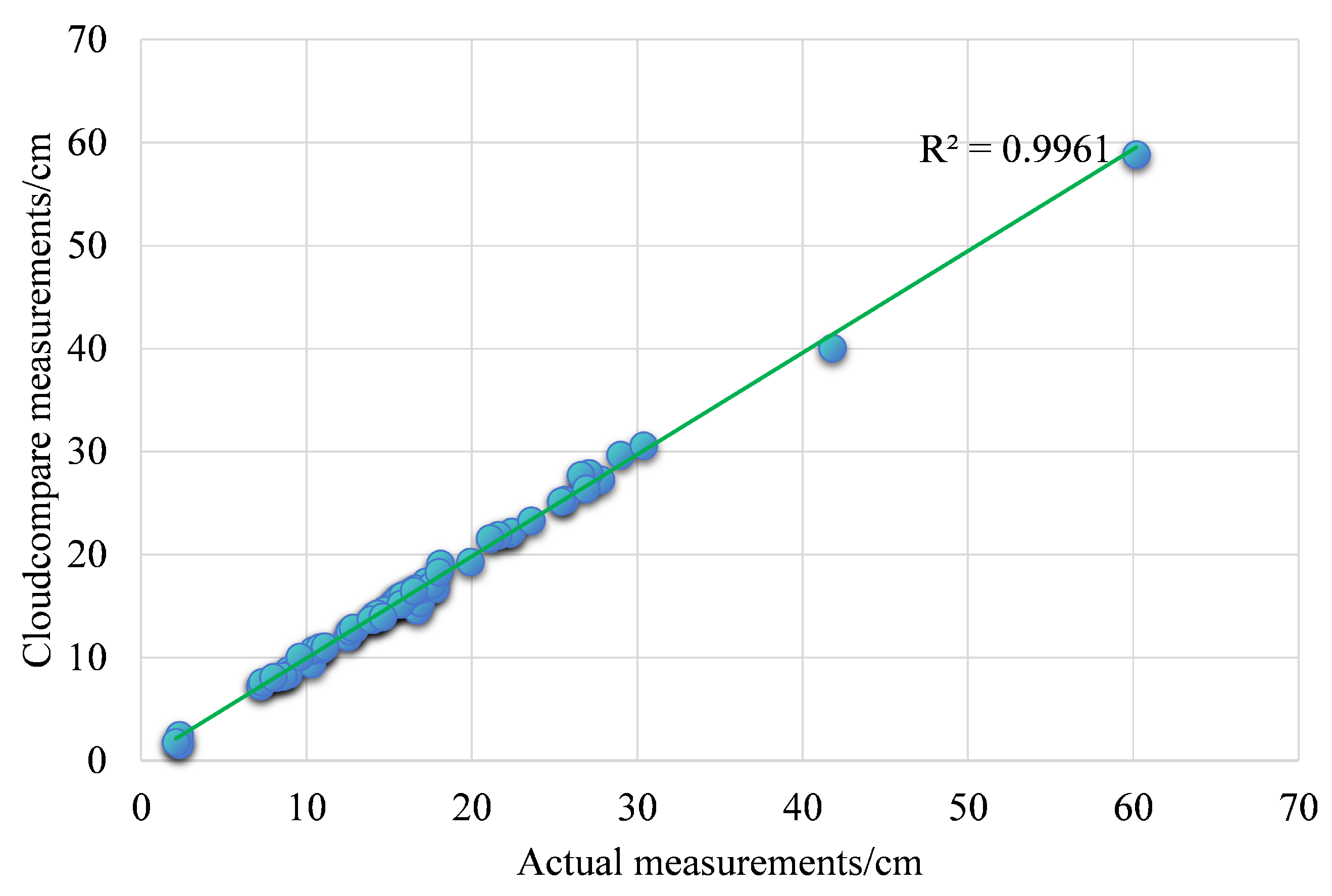
In the data acquisition phase, a tree diameter measurement method is employed to measure the diameter at breast height (DBH). At a height of 1.3 m above the ground, a tape measure is tightly wrapped around the tree trunk to measure the circumference, with three measurements taken to calculate the average. The corresponding diameter is then derived, resulting in a total of 65 valid DBH data points. After individual tree segmentation, CloudCompare software, Version 2.13.beta, is used to measure the 65 trees with accurate DBH data. The real DBH values are compared with those measured by the software to verify the accuracy of the ground-based laser scanner. To quantify this error, the study calculates the mean absolute relative error as in Equation (16).

$$\mathrm{Mean}\mathrm{absolute}\mathrm{relative}\mathrm{error}={\displaystyle \frac{1}{n}}\sum _{i=1}^n\left|{\displaystyle \frac{{\mathrm{Measurements}}_i-\mathrm{True}{\mathrm{value}}_i}{\mathrm{True}{\mathrm{value}}_i}}\right|$$

(16)

where, n represents the total number of samples, and i is the index of the data points.

The relative errors of various samples are shown in

Table 3. Reconstruction accuracy analysis.

Sample Plot	Relative Error/mm
A	0.40
B	0.17
C	0.21
D	0.21
E	0.41
Overall average	0.28

. The calculated overall average relative error is only 0.28 mm. The accuracy of the full scanner has reached the millimeter level, ensuring that a quantitative structural model based on high-precision point cloud data can be constructed. The comparison results are shown in Figure 6, and R² reaches above 0.99.

3.2. Clustering Results of Hickory Tree Structure

3.2.1. Principal Component Analysis

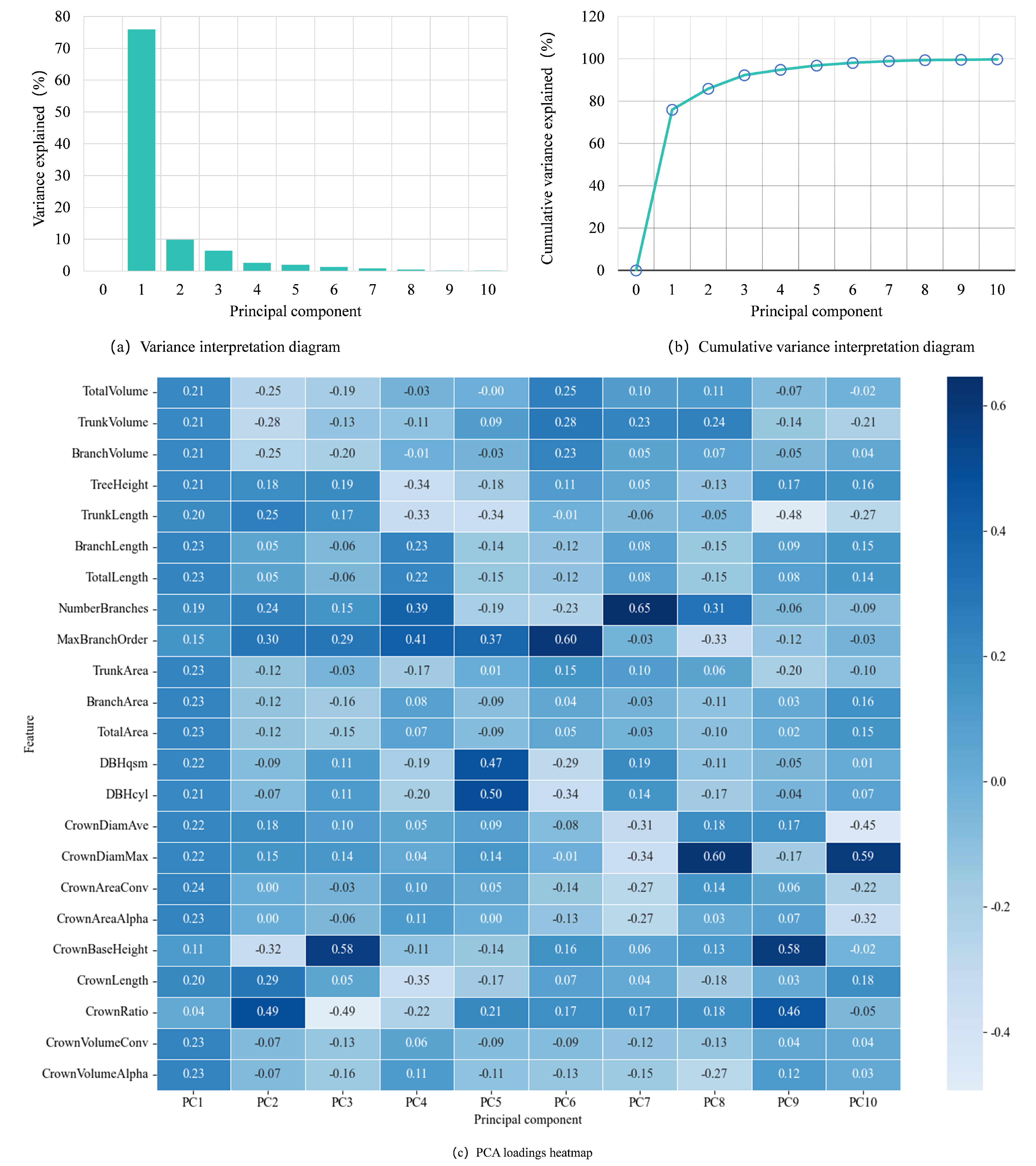
PCA was first applied to the original dataset to reduce its dimensionality. By analyzing the variance contributions of each principal component, as shown in Figure 7, it is observed that the first principal component explains 75.96% of the total variance, indicating that it is the primary source of variation in the data. The second principal component explains an additional 9.90% of the total variance, a relatively small proportion, but it still provides insight into the secondary variation in the data. Together, the first two principal components account for 85.86% of the total variance, a significant proportion that suggests these components capture the most crucial information in the data. By selecting these two principal components for dimensionality reduction, not only is the complexity of the data significantly reduced, which eases the computational burden of the model, but the most valuable features of the data are retained, providing a clearer and more streamlined feature space for subsequent data analysis and model development.

The PCA loadings heatmap illustrates the contributions of individual features to principal components, where the magnitude of each loading reflects its relative importance. Features with larger absolute loadings exert stronger influences on component interpretation, effectively highlighting the most influential features in dimensionality reduction. Notably, the heatmap reveals distinct contribution patterns across components. For the first principal component (PC1), features demonstrate relatively balanced contributions, suggesting a collective influence on this axis. For the second principal component (PC2), three features (CrownRatio, MaxBranchOrder, and CrownLength) exhibit significantly larger absolute loadings compared to others, establishing them as dominant drivers of variance captured by PC2.

3.2.2. K-Means Clustering

After determining the appropriate number of principal components, the data was reduced to two-dimensional space, and the K-means clustering algorithm was applied to identify the clustering structure within the data. The dimensionality reduction not only enhances computational efficiency but also, by focusing on the most important features, enables the K-means algorithm to more clearly identify patterns and structures within the data, thereby improving both clustering accuracy and efficiency. Furthermore, dimensionality reduction makes the clustering results easier to visualize and interpret, aiding in the understanding of the underlying patterns in the data.

Figure 8 shows the results of applying the K-means algorithm to the data with K values set to 2 and 3. By comparing the clustering results for these three different values of K, significant differences in the clustering outcomes can be observed: when K = 3, the distribution of points among the clusters is uneven, with cluster sizes of 51, 28, and 2, where the smallest cluster contains only 2 points. When K = 2, the point distribution between Cluster 0 and Cluster 1 is more balanced, with 46 and 35 points, respectively, and no extremely small clusters are present. Setting K = 2 leads to a more balanced point distribution and eliminates the issue of very small clusters, which helps improve the stability and interpretability of the clustering results.

3.3. Classification Model of Superior Hickory Trees

3.3.1. Building Individual and Crowd Models

Based on the results of the K-means clustering analysis, the data is divided into two categories, and two models are constructed: the individual model and the consensus model. To convert the 4-point scale into a binary classification, a threshold of 2.5 is selected. Scores higher than 2.5 (i.e., 3 and 4 points) are classified as “superior”, labeled as 0 (False), while scores lower than 2.5 (i.e., 1 and 2 points) are classified as “non-superior”, labeled as 1 (True). The ratings of each forest farmer for 81 trees are then converted into binary classification data. For each forest farmer, a binary classification model is constructed, based on their personal rating data, which primarily captures the individual’s judgment and preference regarding the dominance status of the trees. For each tree, the most frequent category (i.e., the mode) among the ratings from 24 forest farmers is calculated to construct a consensus model. The output of this model reflects the collective judgment of the 24 forest farmers, offering higher reliability and representativeness, and better reflecting the consensus of the forest farming community.

3.3.2. Model Accuracy Analysis

This study employed a randomized search framework combined with LOOCV to select best hyper-parameters for the GBDT model. The hyper-parameter search space encompassed critical parameters including: number of trees (50–300), learning rate (uniformly sampled from 0.01 to 0.2), and maximum depth (3–15). A total of 200 hyper-parameter combinations were randomly sampled from the parameter space. Each combination’s generalization performance was evaluated through LOOCV, with classification accuracy serving as the optimization criterion. The final selection prioritized the hyper-parameter configuration achieving the highest mean LOOCV accuracy.

After processing the 72 training samples using LOOCV and determining the optimal hyperparameters for both the individual model and the consensus model, the overall performance of the models is evaluated using three key metrics: LOOCV average accuracy, the score of the best model on the training set, and accuracy. The results are presented in Appendix A,

Table A2. Assessment results of crowd and individual models on the training and test set.

Model	LOOCV Accuracy	Training Accuracy	Test Accuracy
Crowd model	0.87	1	0.78
Forest farmer 1	0.82	1	0.63
Forest farmer 2	0.72	1	0.67
Forest farmer 3	0.82	1	0.67
Forest farmer 4	0.74	0.98	0.67
Forest farmer 5	0.66	1	0.78
Forest farmer 6	0.6	1	0.78
Forest farmer 7	0.86	1	0.89
Forest farmer 8	0.7	0.98	0.78
Forest farmer 9	0.8	1	0.78
Forest farmer 10	0.92	1	0.67
Forest farmer 11	0.76	1	0.56
Forest farmer 12	0.56	1	0.67
Forest farmer 13	0.94	1	0.78
Forest farmer 14	0.72	1	0.67
Forest farmer 15	0.68	1	0.75
Forest farmer 16	0.74	1	0.78
Forest farmer 17	0.66	1	0.89
Forest farmer 18	0.74	1	0.67
Forest farmer 19	0.78	1	0.67
Forest farmer 20	0.74	0.86	0.67
Forest farmer 21	0.74	1	0.78
Forest farmer 22	0.7	1	0.78
Forest farmer 23	0.86	1	0.89
Forest farmer 24	0.76	1	0.67

. The consensus model achieved an LOOCV average accuracy of 87%, a training set accuracy of 100%, and a test set accuracy of 78%. For the individual model, the LOOCV average accuracy reached 75%, with an average training set accuracy exceeding 99%, and an average test set accuracy of over 73%. While the individual model demonstrates a very high average accuracy on the training set, its average accuracy on the test set is relatively lower, indicating some degree of overfitting. However, the objective of constructing the GBDT model in this study is not to develop an accurate classification model, but rather to intentionally allow it to overfit in order to maximize the extraction of information from the data. This approach helps achieve the research goal of identifying commonalities across all individual models and gaining deeper insights into the experiences of the forest farmers.

3.3.3. Analysis and Comparison Based on Crowd Model

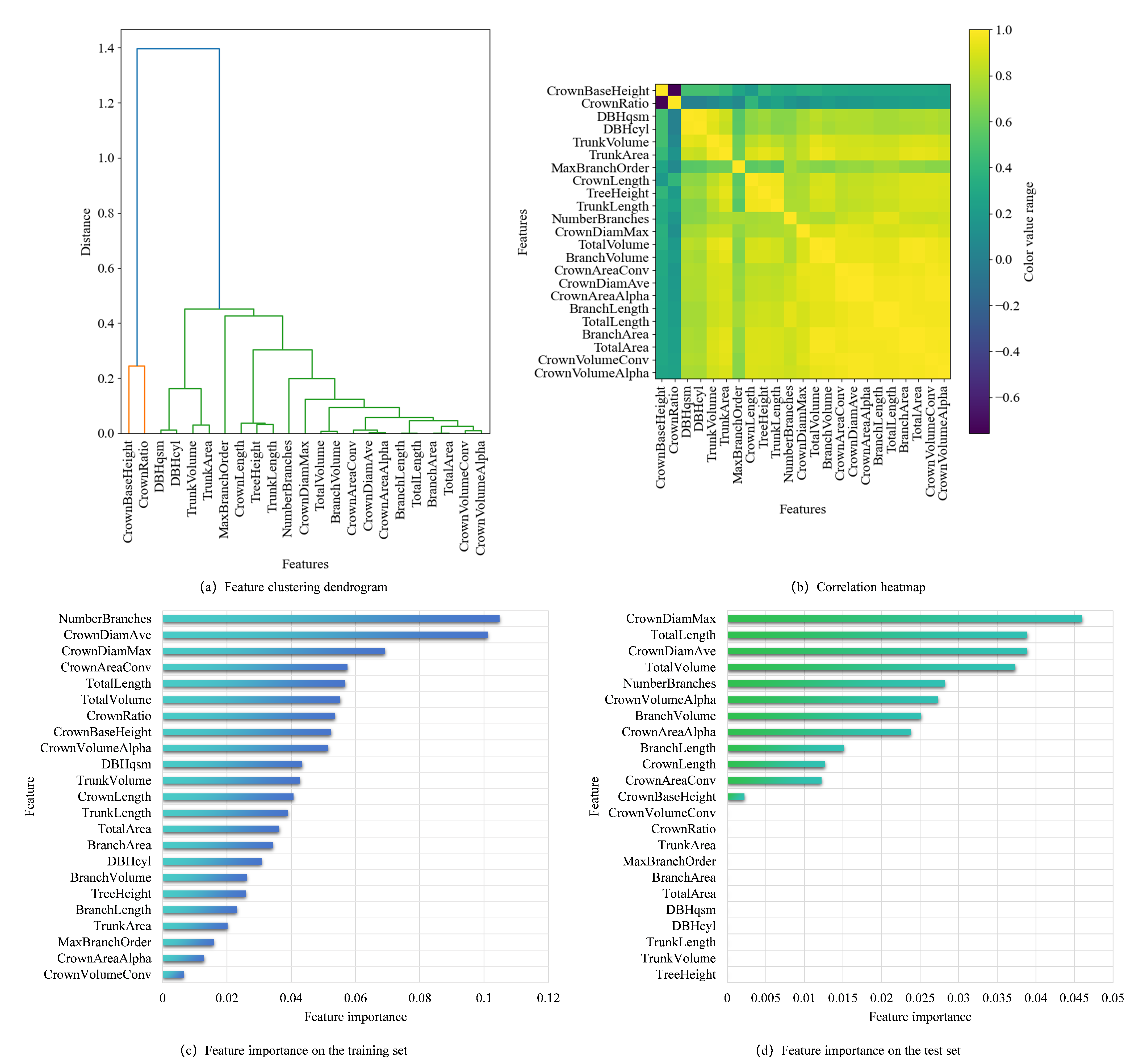
Figure 9 combines hierarchical clustering, correlation patterns, and consensus model-driven importance rankings to holistically evaluate feature relationships and predictive relevance. The dendrogram reveals distinct groupings: CrownBaseHeight forms an isolated cluster, indicating uniqueness, while TrunkVolume and TrunkArea cluster tightly, suggesting shared attributes. The heatmap identifies TrunkVolume and TotalVolume as perfectly correlated, CrownBaseHeight and BranchArea as negatively correlated, and crown-related features (CrownDiamMax, CrownDiamAve) with moderate-to-strong positive correlations (0.6–0.8).

From Figure 9, based on the feature importance ranking in the consensus model for the training set according to the Gini importance metric, the top five features are branch count, average crown diameter, maximum horizontal crown diameter, total length of all branches, and the overall tree volume. Based on the feature importance ranking in the consensus model for the test set according to the permutation importance metric, the top five features are maximum horizontal crown diameter, total length of all branches, average crown diameter, branch count, and overall tree volume.

After calculating the feature importance, the decision nodes of each tree in the GBDT model were analyzed (see

Table 4. GBDT decision thresholds.

Feature	Count	Avg_Threshold	Mid_Threshold	Mode_Threshold	Max_Threshold	Min_Threshold
TotalVolume	111	233.36	205.55	161.75	642.75	32.68
TrunkVolume	110	58.59	48.63	127.15	133.55	8.24
BranchVolume	106	173.61	112.09	102.43	520.75	23.77
TreeHeight	109	7.50	7.89	5.20	11.26	4.72
TrunkLength	115	7.16	7.22	4.02	11.91	3.35
BranchLength	117	404.01	399.35	227.65	889.65	32.48
TotalLength	97	378.25	384.80	571.85	950.00	35.58
NumberBranches	96	1100.80	1097.25	359.00	2009.50	62.50
MaxBranchOrder	55	6.65	6.50	6.50	7.50	5.50
TrunkArea	120	1.95	1.94	2.40	3.34	0.65
BranchArea	105	24.09	22.10	35.35	60.00	3.30
TotalArea	115	25.30	22.82	29.53	60.98	3.90
DBHqsm	105	0.14	0.14	0.14	0.25	0.04
DBHcyl	102	0.13	0.12	0.08	0.24	0.04
CrownDiamAve	126	5.18	5.44	3.29	8.19	2.44
CrownDiamMax	155	6.41	6.39	3.97	9.20	2.95
CrownAreaConv	94	30.28	30.56	10.55	55.49	3.50
CrownAreaAlpha	102	23.71	23.74	28.33	52.14	2.51
CrownBaseHeight	160	1.13	1.26	1.29	1.77	0.32
CrownLength	121	6.75	6.82	5.86	9.89	3.07
CrownRatio	160	0.88	0.88	0.93	0.96	0.75
CrownVolumeConv	77	117.97	106.00	27.89	307.60	4.22
CrownVolumeAlpha	106	88.65	84.49	84.49	251.00	8.81

). The frequency of each feature’s occurrence across all trees, along with their corresponding thresholds, were recorded. The average, median, mode, maximum, and minimum values of these thresholds were then computed. These values provide a general understanding of the importance of each feature. If a feature frequently appears in many decision trees, it likely plays an important role in the model’s decision-making process. The average and median of the thresholds provide typical values for feature-based data splits, while the mode represents the most frequent threshold in the decision trees, indicating the model’s decisions at specific feature values. The maximum and minimum threshold values offer insights into the range of feature values, helping to understand the feature’s distribution. Specifically, if the threshold range for a feature is narrow, with the maximum and minimum values being close, it may suggest that the feature has a stable decision boundary, significantly influencing the model’s predictions. In contrast, a broad threshold range may indicate that the feature is used to capture different data patterns in various decision trees.

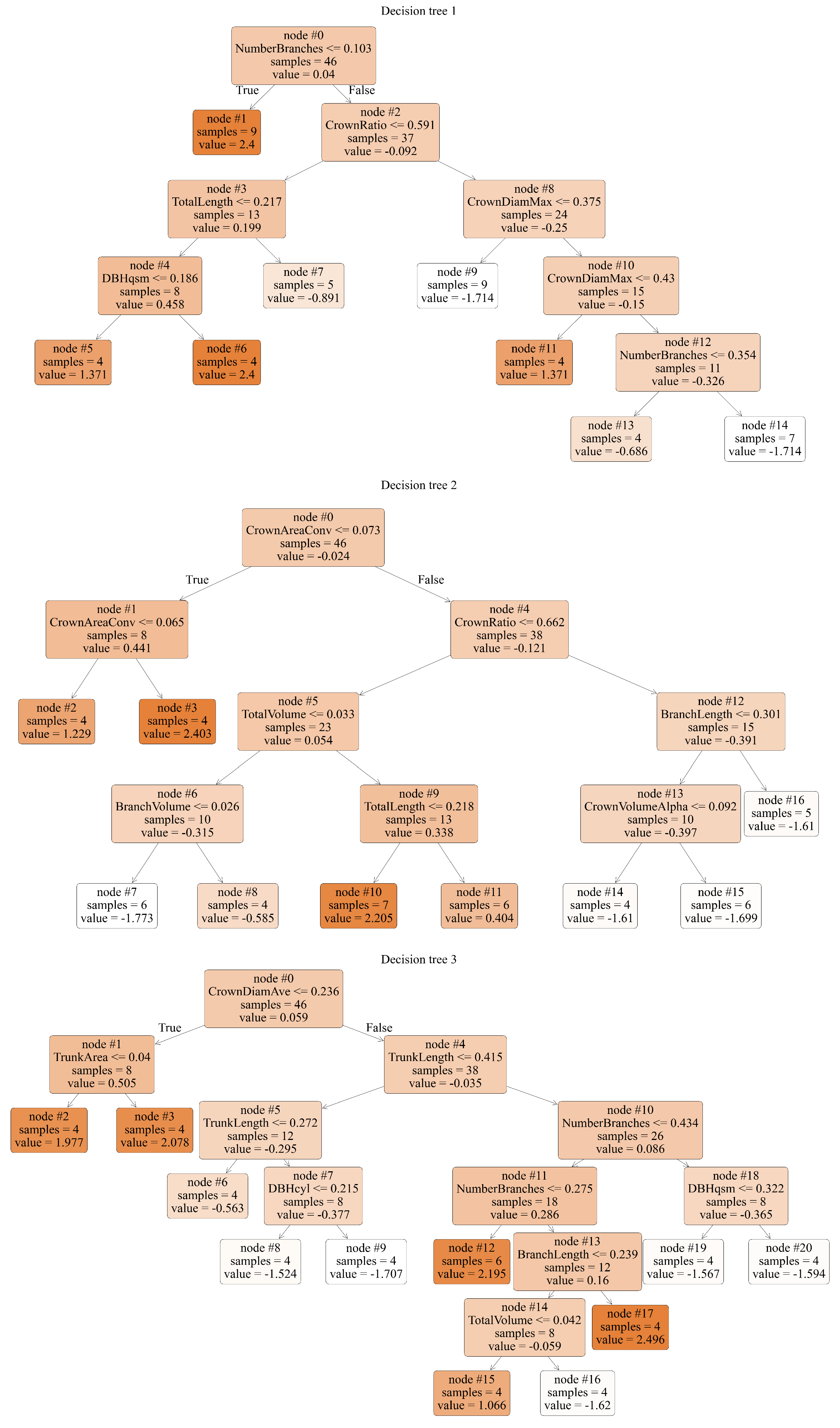
To effectively illustrate the decision process and internal structure of the GBDT model, Figure 10 selectively shows the first three decision trees. As the GBDT model consists of multiple decision trees, each tree corrects the errors of the previous one. The first three trees reveal both the initial predictions made by the model and the subsequent error correction process. These three trees not only represent the model’s initial state but also demonstrate how the model gradually improves its predictive ability. In the visualization of the decision trees, nodes labeled “False” represent superior trees, while nodes labeled “True” are identified as non-superior trees. The node parameter represents decision points in the process, containing the feature and threshold used to split the data. The value parameter indicates the number of samples for each category at each node, aiding in the identification of the data distribution in the tree. The samples parameter shows the total number of samples at each node, reflecting the degree of data segmentation and concentration in the tree.

The most accurate method for determining feature importance is to directly extract feature importance indicators from the model. Based on the frequency of occurrences and threshold statistics, the dominance or non-dominance of trees is then determined. The top five features for both the training and test set rankings in the consensus model are branch count, average crown diameter, maximum horizontal crown diameter, total length of all branches, and overall tree volume. The maximum horizontal crown diameter and average crown diameter appear most frequently in the GBDT model, followed by branch count and total length of all branches. The threshold range (difference between the maximum and minimum values) for the maximum horizontal crown diameter, average crown diameter, branch count, and total length of all branches shows a larger variation compared to the overall tree volume. Although the overall tree volume does not appear the most frequently, its average, median, and mode threshold values are relatively low, suggesting that it may be an important decision factor.

3.3.4. Analysis and Comparison Based on Personal Models

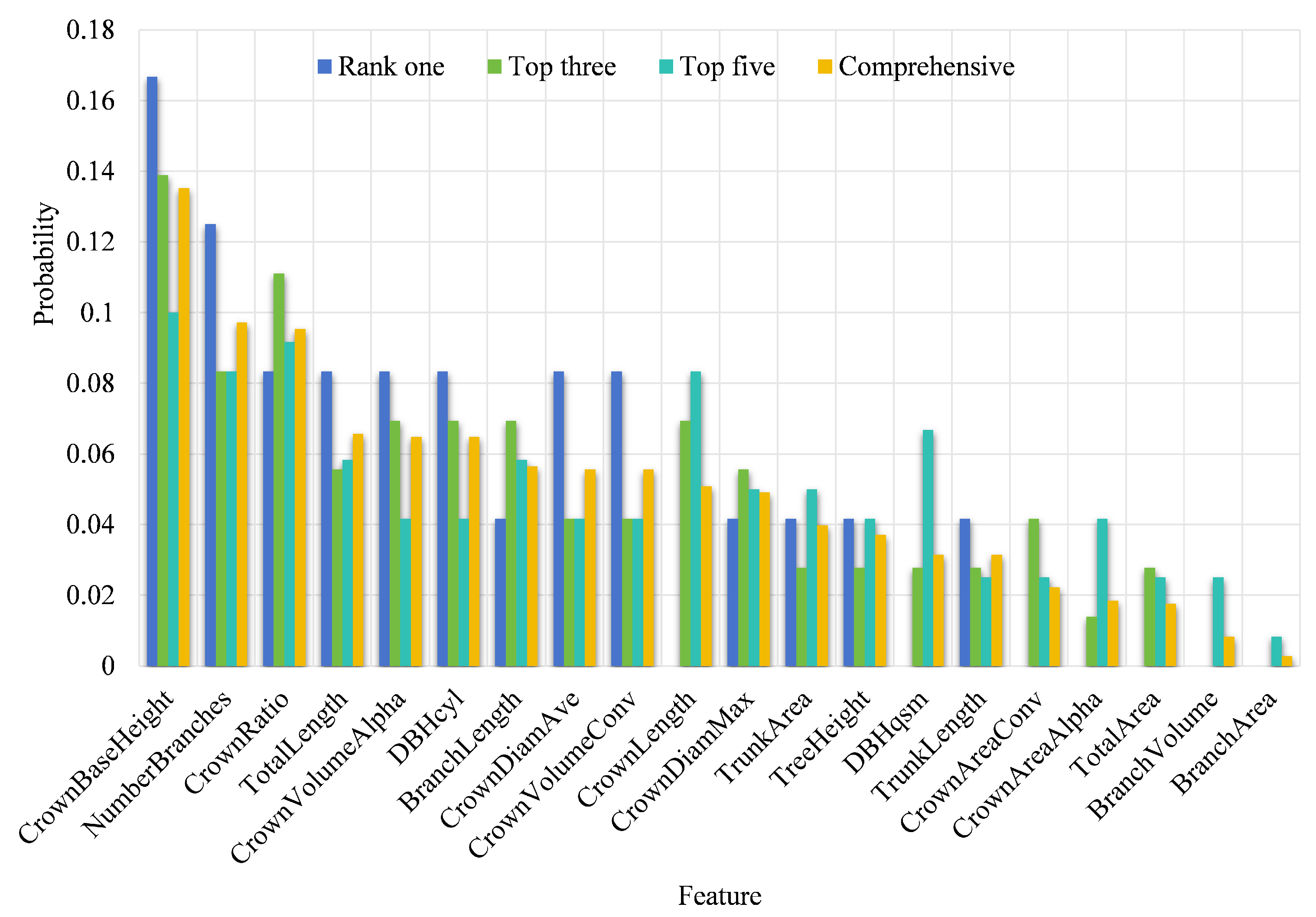
To conduct a more in-depth examination of the distinctions among various features within individual models, we evaluated the first, top three, and top five features for each model. Subsequently, we computed the proportion of these features across all individual models, designating this proportion as the probability value of the feature. Consequently, each feature will yield three aforementioned probability values, and the average of these values will be utilized to derive a comprehensive probability. Figure 11 illustrates the ranking of features based on the comprehensive probability values (represented by the yellow bar chart), arranged in descending order. According to Figure 11, the top four features are height from the ground to crown base, branch count, the ratio of crown length to tree height, and total length of all branches. The fifth position is shared by the volume of the tree’s crown Alpha shape and the tree diameter at 1.1–1.5 m.

When sorted by the probability for the first rank, the top two features are height from the ground to crown base and branch count, followed by the ratio of crown length to tree height, total length of all branches, volume of the tree’s crown Alpha shape, tree diameter at 1.1–1.5 m, average crown diameter, and the volume of the tree crown convex hull.

3.3.5. Analysis of the Differences Between the Crowd Model and the Individual Model

To obtain the expert rating data, this study presented the QSM reconstruction results of individual tree point clouds to experts, displaying images from four different angles. This survey format allows for an intuitive presentation of tree shape features, but it also has limitations. The display angles and visual effects may influence the experts’ ratings, which could, to some extent, affect the assessment of feature importance in the model. The results from both the consensus model and the individual model indicate that tree structural parameters are important for prediction, but there are differences in which specific parameters are most important and to what extent.

On the common aspects, branch count and total length of all branches were identified as important features in both models. This suggests that these features are universally significant for the model’s predictions and are clearly reflected in the images from various angles. Consequently, experts generally rated their importance as high. On the differing aspects, features such as the height from the ground to the crown base, the ratio of crown length to tree height, the volume of the tree’s crown Alpha shape, and the diameter of the tree at 1.1–1.5 m were considered more important in the individual model. However, they did not make it into the top five in the consensus model. This could be because the visual differences of these features across the four image angles were not prominent enough, which led experts to assign them lower importance during individual rating. As a result, they were not frequently rated as important features in the mode-based statistic. In contrast, features such as average crown diameter, maximum horizontal crown diameter, and overall tree volume were considered highly important in the consensus model but did not appear in the individual model. This may be because these features were more consistently and prominently displayed across different image angles, which allowed experts to better recognize their predictive value for tree dominance status, leading them to be frequently rated as important features in the consensus model.

The limitations of the survey data collection format influenced the evaluation of feature importance to some extent, resulting in differences in feature importance rankings between the individual and consensus models. Branch count and total length of all branches were recognized as important features in both models and significantly impacted the model’s prediction results. The height from the ground to crown base exhibited strong predictive capability in the individual model’s dataset. In conclusion, branch count, total length of all branches, and height from the ground to the crown base are the three most significant features affecting the dominance status of Carya cathayensis trees. Combining the decision tree thresholds, a tree can be considered superior if the branch count is greater than 1100.80, the total length of all branches exceeds 378.25 m, and the height from the ground to the crown base is greater than 1.13 m.

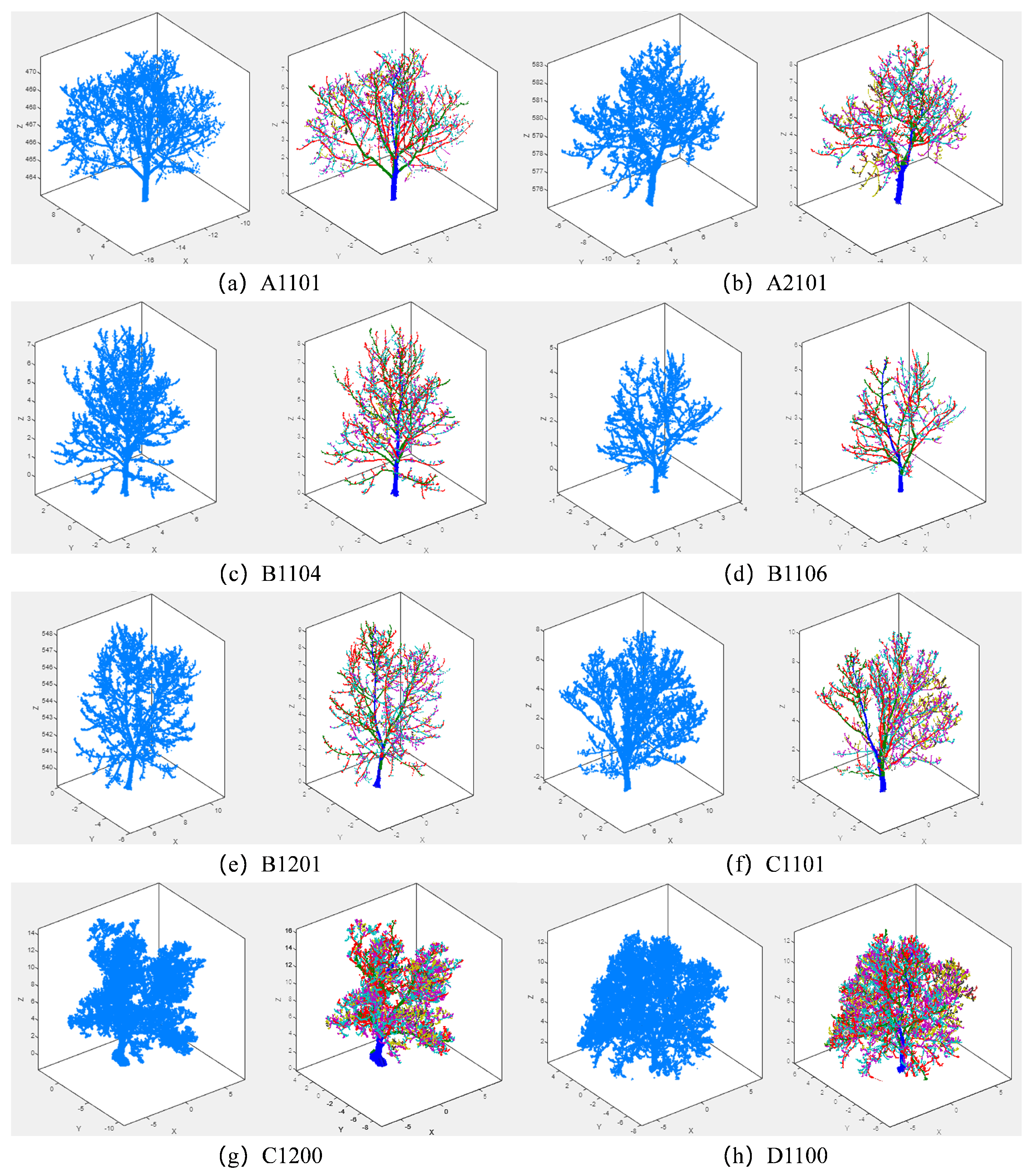
3.4. Analysis of Superior Tree Structure Based on Natural Selection

According to the results of the “Carya Cathayensis Tree King” selection event organized by the Lin’an District Agricultural and Rural Bureau and the District Media Center, the first “Carya Cathayensis Tree King” is located in YinKeng Village, Daoshi Town, with the tree numbered C1200 and an age of 152 years. D1100 is another Tree King located in Longgang Town, with a tree age of 40 years. The location of these Tree Kings has deep soil layers and good soil quality, combined with proper management, allowing them to remain vigorous and productive year after year. They have significant reference value for analyzing optimal tree structure and can be considered as the ideal tree form.

Table 5. Distance metric analysis results.

Optimal Tree	Euclidean Distance				Manhattan Distance
	With the Superior Tree		With Non-Superior Tree		With the Superior Tree		With Non-Superior Tree
	Mean	Range	Mean	Range	Mean	Range	Mean	Range
C1200	2.77	1.22–3.43	3.1	2.26–3.93	12.55	8.10–15.65	13.57	4.54–18.23
D1100	3.43	1.22–4.05	3.73	3.00–4.48	15.56	4.24–18.79	17.15	13.41–21.24

presents the analysis results of the two optimal trees’ structural parameters compared to other trees, based on distance metrics. Specifically, it calculates the Euclidean and Manhattan distances using expert classification labels (excluding the two optimal trees, with 45 remaining superior trees and 34 non-superior trees). By observing the Euclidean and Manhattan distance data between the two optimal trees and the superior and non-superior trees, it is apparent that the distance range between the superior trees and the optimal trees is generally lower than that between the non-superior trees and the optimal trees.

Therefore, a threshold can be set to classify trees within a certain range as superior, while those exceeding this range can be classified as non-superior. For the second optimal tree, the threshold can be set between the two average values; for the first optimal tree, a lower threshold can be considered. After comprehensive consideration, the Euclidean distance threshold is set between 3.0 and 3.5, while the Manhattan distance threshold is set between 13.0 and 16.0. Trees within this range can be considered superior, while those outside this range are considered non-superior. This threshold is determined based on the middle value of the average distances between the two optimal trees and the superior and non-superior trees.

4. Conclusions

This study, based on a comparative analysis of the individual and consensus models, delves deeply into the key structural parameters that influence the Carya cathayensis tree form. Branch count and total branch length, identified as important features by both models, significantly impact prediction results, highlighting the critical role of branch structure in the complexity of tree growth. The height from the ground to the crown base ranked first in probability and combined probability in the individual model, demonstrating a stronger predictive ability within the dataset of the individual model. Branch count, total branch length, and the height from the ground to the crown base can be regarded as the most significant structural parameters affecting the Carya cathayensis tree form. Specifically, when the branch count exceeds 1101, the total branch length exceeds 378 m, and the height from the ground to the crown base exceeds 1 m, these trees can be marked as superior. These findings provide a scientific basis for the accurate assessment and management of Carya cathayensis trees, contributing to more efficient resource allocation and tree care strategies. With these quantifiable standards, researchers and managers can more precisely identify and cultivate trees with growth advantages, thereby improving overall forestry production efficiency and ecological value.

This study also cleverly extends the application of two traditional vector space distance metrics, Euclidean distance and Manhattan distance, to tree structure similarity assessment. By setting thresholds—Euclidean distance between 3.0 and 3.5 and Manhattan distance between 13.0 and 16.0—a clear boundary is established for tree classification. Trees within this range are considered superior, while those outside the range are classified as non-superior. This innovative approach breaks the conventional limitation of distance metrics, which typically apply only to regular vector spaces. Through appropriate transformation and method optimization, these metrics were successfully adapted to the complex and variable characteristics of tree structures. This opens a new perspective for tree shape structure comparison and expands the application boundaries of distance metrics, showcasing the tremendous potential and value of cross-disciplinary knowledge integration.

This study has several limitations and future directions. First, the current survey method using 2D images limits the comprehensive understanding of tree shape features, and future work could use 3D models or cross-sectional views for clearer feature evaluation. Second, the reliance on Euclidean and Manhattan distances for tree structure similarity analysis may not fully capture complex similarities, so future research could incorporate multidimensional metrics like cosine similarity. Third, the model’s predictions lack sufficient real-world validation, and field investigations could help compare predicted and actual yields for improved model accuracy. Lastly, developing intuitive visualization tools to present complex data and enhance model interpretability would make the results more accessible to non-experts and support more efficient forestry management.

References

1. Xiang, L.; Wang, Y.; Yi, X.; Wang, X.; He, X. Chemical constituent and antioxidant activity of the husk of Chinese hickory. J. Funct. Foods 2016, 23, 378–388. [Google Scholar] [CrossRef]
2. Coupel-Ledru, A.; Pallas, B.; Delalande, M.; Segura, V.; Guitton, B.; Muranty, H.; Durel, C.E.; Regnard, J.L.; Costes, E. Tree architecture, light interception and water-use related traits are controlled by different genomic regions in an apple tree core collection. New Phytol. 2022, 234, 209–226. [Google Scholar] [CrossRef] [PubMed]
3. Xu, S.; McVicar, T.R.; Li, L.; Yu, Z.; Jiang, P.; Zhang, Y.; Ban, Z.; Xing, W.; Dong, N.; Zhang, H.; et al. Globally assessing the hysteresis between sub-diurnal actual evaporation and vapor pressure deficit at the ecosystem scale: Patterns and mechanisms. Agric. For. Meteorol. 2022, 323, 109085. [Google Scholar] [CrossRef]
4. Abdolahipour, M.; Kamgar-Haghighi, A.A.; Sepaskhah, A.R.; Zand-Parsa, S.; Honar, T.; Razzaghi, F. Time and amount of supplemental irrigation at different distances from tree trunks influence on morphological characteristics and physiological responses of rainfed fig trees under drought conditions. Sci. Hortic. 2019, 253, 241–254. [Google Scholar] [CrossRef]
5. Schiessl, S.V.; Huettel, B.; Kuehn, D.; Reinhardt, R.; Snowdon, R.J. Flowering time gene variation in Brassica species shows evolutionary principles. Front. Plant Sci. 2017, 8, 1742. [Google Scholar] [CrossRef]
6. Hansen, M.C.; Potapov, P.V.; Moore, R.; Hancher, M.; Turubanova, S.A.; Tyukavina, A.; Thau, D.; Stehman, S.V.; Goetz, S.J.; Loveland, T.R.; et al. High-resolution global maps of 21st-century forest cover change. Science 2013, 342, 850–853. [Google Scholar] [CrossRef]
7. White, J.C.; Coops, N.C.; Wulder, M.A.; Vastaranta, M.; Hilker, T.; Tompalski, P. Remote sensing technologies for enhancing forest inventories: A review. Can. J. Remote Sens. 2016, 42, 619–641. [Google Scholar] [CrossRef]
8. Talucci, A.C.; Forbath, E.; Kropp, H.; Alexander, H.D.; DeMarco, J.; Paulson, A.K.; Zimov, N.S.; Zimov, S.; Loranty, M.M. Evaluating post-fire vegetation recovery in Cajander Larch Forests in Northeastern Siberia using UAV derived vegetation indices. Remote Sens. 2020, 12, 2970. [Google Scholar] [CrossRef]
9. Wang, Z.; Zhang, L.; Fang, T.; Mathiopoulos, P.T.; Qu, H.; Chen, D.; Wang, Y. A structure-aware global optimization method for reconstructing 3-D tree models from terrestrial laser scanning data. IEEE Trans. Geosci. Remote Sens. 2014, 52, 5653–5669. [Google Scholar] [CrossRef]
10. Crommelinck, S.; Höfle, B. Simulating an autonomously operating low-cost static terrestrial LiDAR for multitemporal maize crop height measurements. Remote Sens. 2016, 8, 205. [Google Scholar] [CrossRef]
11. Kükenbrink, D.; Marty, M.; Bösch, R.; Ginzler, C. Benchmarking laser scanning and terrestrial photogrammetry to extract forest inventory parameters in a complex temperate forest. Int. J. Appl. Earth Obs. Geoinf. 2022, 113, 102999. [Google Scholar] [CrossRef]
12. Brolly, G.; Király, G.; Lehtomäki, M.; Liang, X. Voxel-based automatic tree detection and parameter retrieval from terrestrial laser scans for plot-wise forest inventory. Remote Sens. 2021, 13, 542. [Google Scholar] [CrossRef]
13. Yrttimaa, T.; Luoma, V.; Saarinen, N.; Kankare, V.; Junttila, S.; Holopainen, M.; Hyyppä, J.; Vastaranta, M. Structural changes in boreal forests can be quantified using terrestrial laser scanning. Remote Sens. 2020, 12, 2672. [Google Scholar] [CrossRef]
14. Shen, X.; Huang, Q.; Wang, X.; Li, J.; Xi, B. A deep learning-based method for extracting standing wood feature parameters from terrestrial laser scanning point clouds of artificially planted forest. Remote Sens. 2022, 14, 3842. [Google Scholar] [CrossRef]
15. Krause, P.; Forbes, B.; Barajas-Ritchie, A.; Clark, M.; Disney, M.; Wilkes, P.; Bentley, L.P. Using terrestrial laser scanning to evaluate non-destructive aboveground biomass allometries in diverse Northern California forests. Front. Remote Sens. 2023, 4, 1132208. [Google Scholar] [CrossRef]
16. Zimbres, B.; Shimbo, J.; Bustamante, M.; Levick, S.; Miranda, S.; Roitman, I.; Silvério, D.; Gomes, L.; Fagg, C.; Alencar, A. Savanna vegetation structure in the Brazilian Cerrado allows for the accurate estimation of aboveground biomass using terrestrial laser scanning. For. Ecol. Manag. 2020, 458, 117798. [Google Scholar] [CrossRef]
17. Goodbody, T.R.; Coops, N.C.; Tompalski, P.; Crawford, P.; Day, K.J. Updating residual stem volume estimates using ALS-and UAV-acquired stereo-photogrammetric point clouds. Int. J. Remote Sens. 2017, 38, 2938–2953. [Google Scholar] [CrossRef]
18. Jiang, R.; Lin, J.; Li, T. Refined aboveground biomass estimation of moso bamboo forest using culm lengths extracted from TLS point cloud. Remote Sens. 2022, 14, 5537. [Google Scholar] [CrossRef]
19. Yusup, A.; Halik, Ü.; Keyimu, M.; Aishan, T.; Abliz, A.; Dilixiati, B.; Wei, J. Trunk volume estimation of irregular shaped Populus euphratica riparian forest using TLS point cloud data and multivariate prediction models. For. Ecosyst. 2023, 10, 100082. [Google Scholar] [CrossRef]
20. Terryn, L.; Calders, K.; Disney, M.; Origo, N.; Malhi, Y.; Newnham, G.; Raumonen, P.; Verbeeck, H. Tree species classification using structural features derived from terrestrial laser scanning. ISPRS J. Photogramm. Remote Sens. 2020, 168, 170–181. [Google Scholar] [CrossRef]
21. Gao, W.; Yang, X.; Cao, L.; Cao, F.; Liu, H.; Qiu, Q.; Shen, M.; Yu, P.; Liu, Y.; Shen, X. Screening of Ginkgo Individuals with Superior Growth Structural Characteristics in Different Genetic Groups Using Terrestrial Laser Scanning (TLS) Data. Plant Phenomics 2023, 5, 0092. [Google Scholar] [CrossRef] [PubMed]
22. Dai, W.; Jiang, Y.; Zeng, W.; Chen, R.; Xu, Y.; Zhu, N.; Xiao, W.; Dong, Z.; Guan, Q. MDC-Net: A multi-directional constrained and prior assisted neural network for wood and leaf separation from terrestrial laser scanning. Int. J. Digit. Earth 2023, 16, 1224–1245. [Google Scholar] [CrossRef]
23. Yang, M.; Zhang, Y.; Xi, B. Visualization Simulation of Branch Fractures Based on Internal Structure Reconstruction. Forests 2023, 14, 1020. [Google Scholar] [CrossRef]
24. Chen, X.; Wang, R.; Shi, W.; Li, X.; Zhu, X.; Wang, X. An individual tree segmentation method that combines LiDAR data and spectral imagery. Forests 2023, 14, 1009. [Google Scholar] [CrossRef]
25. Huang, H.; Tian, G.; Chen, C. Evaluating the point cloud of individual trees generated from images based on Neural Radiance fields (NeRF) method. Remote Sens. 2024, 16, 967. [Google Scholar] [CrossRef]
26. Wu, S.; Wen, W.; Wang, Y.; Fan, J.; Wang, C.; Gou, W.; Guo, X. MVS-Pheno: A portable and low-cost phenotyping platform for maize shoots using multiview stereo 3D reconstruction. Plant Phenomics 2020, 2020, 1848437. [Google Scholar] [CrossRef]
27. Isokane, T.; Okura, F.; Ide, A.; Matsushita, Y.; Yagi, Y. Probabilistic plant modeling via multi-view image-to-image translation. In Proceedings of the IEEE Conference on Computer Vision and Pattern Recognition, Salt Lake City, UT, USA, 18–23 June 2018; pp. 2906–2915. [Google Scholar]
28. Gao, T.; Zhu, F.; Paul, P.; Sandhu, J.; Doku, H.A.; Sun, J.; Pan, Y.; Staswick, P.; Walia, H.; Yu, H. Novel 3D imaging systems for high-throughput phenotyping of plants. Remote Sens. 2021, 13, 2113. [Google Scholar] [CrossRef]
29. Liu, Y.; Zhang, A.; Gao, P. From Crown Detection to Boundary Segmentation: Advancing Forest Analytics with Enhanced YOLO Model and Airborne LiDAR Point Clouds. Forests 2025, 16, 248. [Google Scholar] [CrossRef]
30. Zhu, D.; Liu, X.; Zheng, Y.; Xu, L.; Huang, Q. Improved tree segmentation algorithm based on backpack-LiDAR point cloud. Forests 2024, 15, 136. [Google Scholar] [CrossRef]
31. Dong, Y.; Fan, G.; Zhou, Z.; Liu, J.; Wang, Y.; Chen, F. Low cost automatic reconstruction of tree structure by AdQSM with terrestrial close-range photogrammetry. Forests 2021, 12, 1020. [Google Scholar] [CrossRef]
32. Du, S.; Lindenbergh, R.; Ledoux, H.; Stoter, J.; Nan, L. AdTree: Accurate, detailed, and automatic modelling of laser-scanned trees. Remote Sens. 2019, 11, 2074. [Google Scholar] [CrossRef]
33. Xie, D.; Wang, X.; Qi, J.; Chen, Y.; Mu, X.; Zhang, W.; Yan, G. Reconstruction of single tree with leaves based on terrestrial LiDAR point cloud data. Remote Sens. 2018, 10, 686. [Google Scholar] [CrossRef]
34. Bailey, B.N.; Ochoa, M.H. Semi-direct tree reconstruction using terrestrial LiDAR point cloud data. Remote Sens. Environ. 2018, 208, 133–144. [Google Scholar] [CrossRef]
35. Zhang, R.; Zhang, Z.; Zhang, W.; He, L.; Zhu, C. Deep learning-driven semantic segmentation and spatial analysis of quarry relic landscapes using point cloud data: Insights from the Shaoxing quarry relics. NPJ Herit. Sci. 2025, 13, 77. [Google Scholar] [CrossRef]
36. Jaafar, H.A.; Meng, X.; Sowter, A.; Bryan, P. New approach for monitoring historic and heritage buildings: Using terrestrial laser scanning and generalised Procrustes analysis. Struct. Control Health Monit. 2017, 24, e1987. [Google Scholar] [CrossRef]
37. Arrizza, S.; Marras, S.; Ferrara, R.; Pellizzaro, G. Terrestrial Laser Scanning (TLS) for tree structure studies: A review of methods for wood-leaf classifications from 3D point clouds. Remote Sens. Appl. Soc. Environ. 2024, 36, 101364. [Google Scholar] [CrossRef]
38. Li, D.; Jia, W.; Li, F.; Guo, H.; Wang, F.; Zhang, X. Assessing effects of thinning on the stem form in larch during the stand initiation and stem exclusion stages using terrestrial laser scanning. Front. For. Glob. Change 2025, 8, 1418334. [Google Scholar] [CrossRef]
39. Calders, K.; Newnham, G.; Burt, A.; Murphy, S.; Raumonen, P.; Herold, M.; Culvenor, D.; Avitabile, V.; Disney, M.; Armston, J.; et al. Nondestructive estimates of above-ground biomass using terrestrial laser scanning. Methods Ecol. Evol. 2015, 6, 198–208. [Google Scholar] [CrossRef]
40. Stovall, A.E.; Shugart, H.H. Improved biomass calibration and validation with terrestrial LiDAR: Implications for future LiDAR and SAR missions. IEEE J. Sel. Top. Appl. Earth Obs. Remote Sens. 2018, 11, 3527–3537. [Google Scholar] [CrossRef]
41. Delagrange, S.; Jauvin, C.; Rochon, P. PypeTree: A tool for reconstructing tree perennial tissues from point clouds. Sensors 2014, 14, 4271–4289. [Google Scholar] [CrossRef]
42. Moorthy, S.M.K.; Raumonen, P.; Van den Bulcke, J.; Calders, K.; Verbeeck, H. Terrestrial laser scanning for non-destructive estimates of liana stem biomass. For. Ecol. Manag. 2020, 456, 117751. [Google Scholar] [CrossRef]
43. Huang, M.; Lu, R.; Wu, Y.; Zhao, T.; Zhao, J.; Ma, L. Spatiotemporal dynamics and influencing factors of soil quality in aeolian desertified lands of the Qinghai-Tibet Plateau. Ecol. Indic. 2025, 172, 113264. [Google Scholar] [CrossRef]
44. Yang, X.; Xiong, J.; Du, T.; Ju, X.; Gan, Y.; Li, S.; Xia, L.; Shen, Y.; Pacenka, S.; Steenhuis, T.S.; et al. Diversifying crop rotation increases food production, reduces net greenhouse gas emissions and improves soil health. Nat. Commun. 2024, 15, 198. [Google Scholar] [CrossRef] [PubMed]
45. Ke, G.; Meng, Q.; Finley, T.; Wang, T.; Chen, W.; Ma, W.; Ye, Q.; Liu, T.Y. Lightgbm: A highly efficient gradient boosting decision tree. Adv. Neural Inf. Process. Syst. 2017, 30, 3149–3157. [Google Scholar]
46. Pang, Y.; Wang, Y.; Lai, X.; Zhang, S.; Liang, P.; Song, X. Enhanced Kriging leave-one-out cross-validation in improving model estimation and optimization. Comput. Methods Appl. Mech. Eng. 2023, 414, 116194. [Google Scholar] [CrossRef]
47. Berger, Y.G.; Balay, İ.G. Confidence intervals of Gini coefficient under unequal probability sampling. J. Off. Stat. 2020, 36, 237–249. [Google Scholar] [CrossRef]
48. Liu, K.; Shang, Y.; Ouyang, Q.; Widanage, W.D. A data-driven approach with uncertainty quantification for predicting future capacities and remaining useful life of lithium-ion battery. IEEE Trans. Ind. Electron. 2020, 68, 3170–3180. [Google Scholar] [CrossRef]
49. Ramosaj, B.; Pauly, M. Consistent and unbiased variable selection under indepedent features using Random Forest permutation importance. Bernoulli 2023, 29, 2101–2118. [Google Scholar] [CrossRef]
50. San Millán-Castillo, R.; Martino, L.; Morgado, E. A variable selection analysis for soundscape emotion modelling using decision tree regression and modern information criteria. IEEE Access 2024, 12, 92622–92634. [Google Scholar] [CrossRef]
Figure 1. Technical flowchart of the proposed method. Each rectangular box denotes a distinct processing state. The black arrows signify the direction of the processing flow, whereas the red arrows indicate the visualization of intermediate outputs at each stage of the process.
Forests 16 00878 g001
Figure 2. Point cloud acquisition.
Forests 16 00878 g002
Figure 3. The results of single wood segmentation.
Forests 16 00878 g003
Figure 4. Visualization of hickory point clouds of different tree ages and corresponding QSM model. The blue trees represent the point clouds, while the colored trees denote the reconstructed trees, with varying colors signifying different branch orders.
Forests 16 00878 g004
Figure 5. Visualization of tree reconstruction results for surveys with each tree encompassing four distinct perspectives.
Forests 16 00878 g005
Figure 6. The result of comparing the measured value of DBH data with the measured value of Cloudcompare.
Forests 16 00878 g006
Figure 7. PCA results.
Forests 16 00878 g007
Figure 8. K-means Clustering result. (a) The number of clusters is 2. (b) The number of clusters is 3.
Forests 16 00878 g008
Figure 9. Feature evaluation results for clustering, correlations, and consensus model based importance. (a) Hierarchical clustering dendrogram of features based on spearman correlation. (b) Spearman correlation matrix of the features. (c) Feature importance according to the Gini impurity metric on the training set. (d) Feature importance according to the permutation importance metric on the test set.
Forests 16 00878 g009
Figure 10. GBDT decision node diagram. Here the first 3 decision trees are displayed. Each rectangle denotes a tree node.
Forests 16 00878 g010
Figure 11. Analysis of feature importance for individual models.
Forests 16 00878 g011