Article

Assessing the Impact of Forest Machinery Passage on Soil CO2 Concentration

1
Department of Forest Harvesting, Logistics and Ameliorations, Faculty of Forestry, Technical University in Zvolen, 96001 Zvolen, Slovakia
2
Department of Forestry Technologies and Construction, Faculty of Forestry and Wood Sciences, Czech University of Life Sciences Prague, 16500 Prague, Czech Republic
3
The Forest Risk Research Centre, Faculty of Forestry and Wood Sciences, Czech University of Life Sciences Prague, 16500 Prague, Czech Republic
4
Department of Biodiversity of Ecosystems and Landscape, Institute of Landscape Ecology, Slovak Academy of Sciences, 94901 Nitra, Slovakia
*
Author to whom correspondence should be addressed.
Forests 2025, 16(6), 1025; https://doi.org/10.3390/f16061025
Submission received: 30 April 2025 / Revised: 10 June 2025 / Accepted: 16 June 2025 / Published: 19 June 2025
(This article belongs to the Section Forest Operations and Engineering)

Abstract

Forestry machinery plays a key role in forest management, but its increasing weight significantly impacts soil condition. Machinery passage causes soil compaction, which alters the physical, chemical, and biological properties of the soil and affects CO2 concentration. This study aimed to measure the impact of soil compaction on the evolution of CO2 concentrations over three years. Research was conducted near Zvolen, Slovakia, where soil was compacted in 2020 by a forestry skidder. The intensity of compaction was evaluated using a digital penetrometer. CO2 concentrations were measured with a Vaisala MI70 device, with 22 measurements taken post-compaction at an average interval of 52 days. Soil compaction was characterized by a derived penetration index. At a depth of 10 cm, the average penetration index was 119%, indicating a 19% increase in resistance. The highest index, 134%, was found at a depth of 3 cm. A correlation of 0.4 was found between the number of passes and CO2 concentration at 30 cm depth, and 0.8 between penetration index and CO2 concentration. Results showed a significant impact of forestry machinery on soil CO2 concentration, even three years later. Therefore, operating practices should minimize machinery impact on forest soils.

1. Introduction

The mechanization of forestry operations is unavoidable because it provides benefits in reducing costs and manual labor and efficient timber production. The passage of forestry machinery causes soil compaction, leading to significant changes in soil structure and moisture content [1,2,3,4]. The severity of soil compaction caused by machinery operation varies depending on the type of forest machine used and applied harvesting method, the frequency of machine operation, and soil characteristics [5,6,7]. The slope of the terrain and the intensity of traffic are the main factors that determine the soil compaction caused by machinery operation [8,9]. It is known that the slope of the terrain has an important influence on the ruts created by forest machinery [10,11].
Poor aeration of soil caused by soil compaction prevents the development of root systems and limits the water permeability of roots [3,12,13]. Concentration of CO2 serves as an indicator of soil degradation caused by forest mechanization [14]. Some works show it is a more sensitive indicator of compaction compared to bulk density and penetration resistance [15]. The concentration of CO2 in the soil organic horizon is only slightly higher than in the atmosphere [2]. As soil depth increases, the CO2 concentration rises [16,17] and is accompanied by a significant reduction in oxygen (O2) levels [18]. Seasonal variations of soil characteristics significantly influence soil CO2 concentrations. The highest soil CO2 concentrations are recorded at the end of summer, while the lowest values occur during winter, demonstrating a pronounced seasonal pattern [1,2]. The balance between CO2 and O2 varies based on the soil water content and biological activity and directly affects root growth [18].
The objective of this study was to examine the impact of soil compaction, induced experimentally using forestry machinery, on soil CO2 concentration. We hypothesized that soil compaction would result in higher soil CO2 concentration. In addition to soil CO2 concentrations, we assessed soil temperature, soil moisture, the number of machinery passes, and soil penetration resistance and analyzed the relationships between soil CO2 concentrations and these observed variables.

2. Materials and Methods

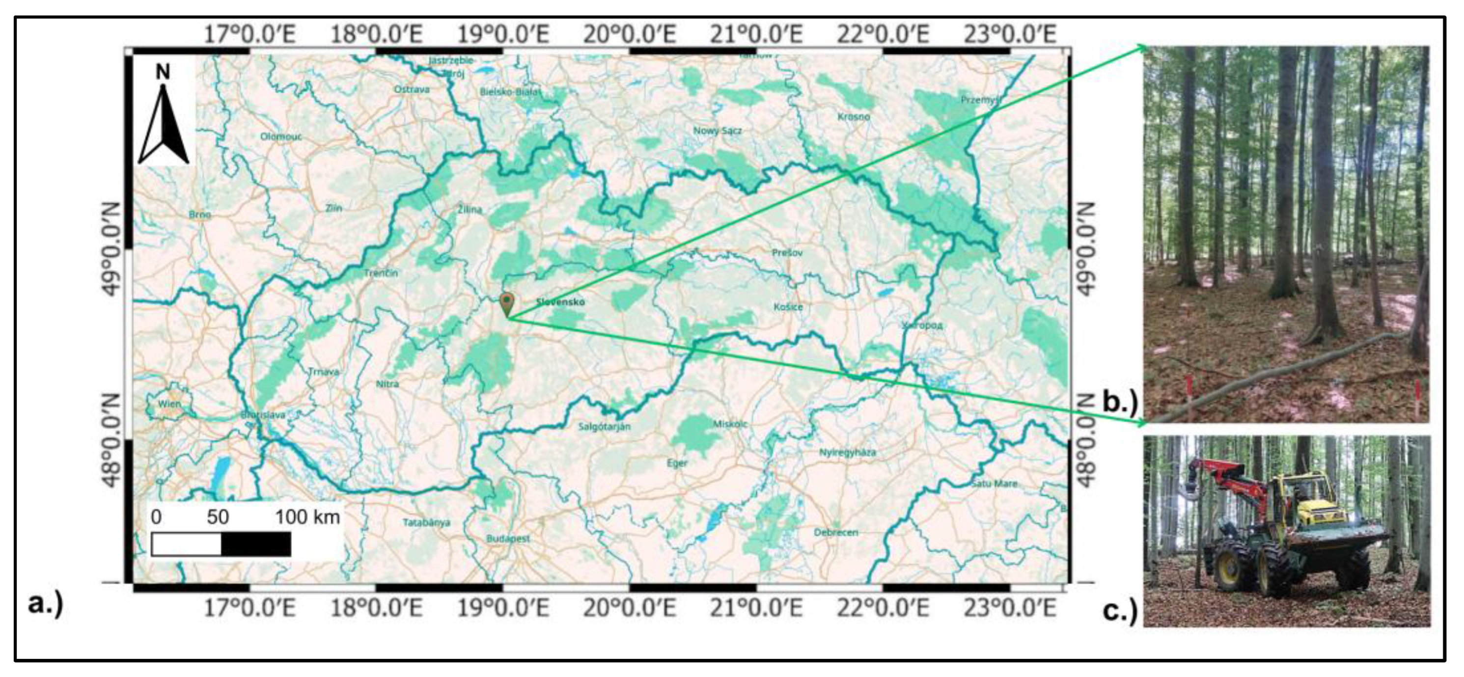
2.1. Site Description

The research site was located within the University Forest Enterprise of the Technical University in Zvolen, Slovakia (Figure 1).
The permanent research plot (PRP) with dimensions 60 × 25 m was established in 2020. Measurements were carried out in stand No. 554 (48°38′35.5″ N 19°02′12.5″ E) at the locality “Stagiar”. Basic stand and site characteristics, along with key soil parameters, are summarized in Table 1. The study area belongs to a moderately cold and very humid climatic region of Slovakia. The long-term mean annual temperature is 6.6 °C. The monthly temperature varies from −4 °C in January to 16 °C in July, and the average annual precipitation is 850 mm [19].

2.2. Experimental Design

The experimental soil compaction was conducted in June 2020. The PRP consists of two sub-plots: a control sub-plot and a compacted sub-plot (treatment with a forestry skidder—LKT 81 ITL was applied). Each sub-plot was 625 m2 large (25 × 25 m). The tractor route within the plot was randomized. The machine drove at a walking pace over the soil surface unloaded to maintain consistent weight during the passage. Both the route and the traffic intensity (i.e., the number of passes) of the tractor were documented manually and recorded using GPS. During the manual drafting of the tractor route, orientation was guided by the positions and numbers of the trees. Given the inaccuracy of the GPS recording, which was affected by the dense tree canopy, a hand-drawn representation was ultimately utilized. The drawing was vectorized and georeferenced using QGIS software version 3.14 [21]. The traffic intensity was described as the number and length of passes within a 1 × 1 m square. Importantly, the compaction process was conducted under controlled experimental conditions and was not a part of a timber harvesting operation. In addition to measuring soil CO2 concentrations, we assessed soil temperature, soil moisture, the number of machinery passes, and soil penetration resistance. Subsequently, we analyzed the relationships between soil CO2 concentrations and these observed variables. Thanks to the three-year duration of the experiment, we were able to investigate the dynamics of soil characteristics, including temperature, moisture, and CO2 concentration, as well as their temporal development following the soil compaction event.
Tire pressure was measured with a Pneurex 1 portable tire pressure regulator (Blitz Co., Ltd., Bräunlingen, Germany). A DINI ARGEO 3590 E axle scale with two WWSE10T load cells (700 × 450 mm; capacity 10,000 kg) was used to determine the machine weight. Technical parameters of the forestry skidder—LKT 81 ITL—are shown in Table 2.

2.3. Soil Physical and Chemical Properties

To determine the soil texture in the forest stand, soil samples were collected and analyzed in the laboratory to quantify the proportion of fine fractions below 0.063 mm (clay, silt, and sand) using the Casagrande method. Soil samples were taken from half of the points at which penetration resistance was measured (Figure 2). Soil samples were collected up to 50 cm deep using steel cylinders (6 cm diameter, 100 cm long) to determine particle size fractions (0–0.25 mm, 0.25–2 mm, 2–4 mm, and >4 mm) at each soil layer defined by the depth. The sampled soil was divided into five layers, each 10 cm wide. After the division, the samples from different soil layers (0–10 cm, 10–20 cm, 20–30 cm, 30–40 cm, and 40–50 cm) were evaluated in the laboratory using the particle size analysis and bulk density test.

2.3.1. Measurement of Soil Penetration Resistance

Penetration resistance (PR) measurements were carried out in June 2020 using a digital penetrometer (Eijkelkamp Penetrologger 0615SA, Giesbeek, The Netherlands) from the Royal Eijkelkamp Company. The penetrometer was equipped with an 80 cm long rod and a cone with a diameter of 11.3 mm, an area of 1 cm2, and an angle of 30°. The penetration rate was 2 cm s−1. The penetrometer was fitted with a new cone before each measurement. The data were first stored in the memory of the instrument, from where they were exported to the computer using the Eijkelkamp Penetroviewer software 6.0. Penetration resistance data were processed in the statistical program R Version x64 4.0.3 [22].
PR values were measured in megapascals (MPa) at 1 cm depth intervals until solid rock was reached. PR values were obtained from both compacted and control sub-plots. At the compacted sub-plot, measurements were taken once before compaction (BC) and once after the compaction (AC) treatment, and the penetration index Equation (1) was calculated based on the difference between these two measurements. The number of measurement points to detect the PR was 100 on both the compacted and control sub-plots in a 2.5 × 2.5 m systematic grid.
Soil compaction was quantified using the penetration index, calculated as follows:
P e n e t r a t i o n   i n d e x = A f t e r   C o m p a c t i o n   ( A C ) B e f o r e   C o m p a c t i o n   ( B C ) × 100
This index represents the relative change in penetration resistance as a result of soil compaction. A value of the penetration index above 100% indicates an increase in resistance, while values close to 100% indicate minimal change. In this study, the penetration index was used to evaluate the impact of soil compaction across various depths within the compacted sub-plot. It enabled a quantitative comparison of soil resistance before and after compaction within the compacted sub-plot.

2.3.2. Carbon Dioxide (CO2) Concentration, Temperature, and Moisture of Soil

The measurements were carried out at the permanent research plot, each time using two probes, one of which was placed in the soil compacted by the passage of a tractor; the other served as a control probe placed in the natural, undisturbed soil. At each sub-plot, 30 points were established near the points that were used for soil sampling. The distribution of points over the research plot followed the principles of stratified sampling, considering canopy coverage and the number of passages at the compacted sub-plot. The points at the control and compacted plots were paired if they were characterized with similar canopy cover and if the distance between them was below 30 m due to technical constraints. A representation of the individual pairs at which CO2 and temperature measurements were made is shown in Figure 3. The measurements were carried out using the Vaisala MI70 instrument and the following probes: the GM70 Carbon Dioxide Probe to measure CO2 concentration and the Vaisala Handheld HM70 Humidity and Temperature Probe to measure soil temperature and relative moisture of soil. Probes for CO2 measurements can detect CO2 concentration in the range of min. 0 to max. 5%. The changes in temperature, relative moisture, and CO2 concentration were measured at the same points within the sub-plots over a period of 3 years after compaction.
At each point, measurements were carried out at soil depths of 10 cm and 30 cm. Temperature and CO2 measurements were performed for all pairs of points at regular time intervals to capture the trend throughout the year (seasonal trend) in order to track differences between the compacted and control sub-plots. The measurement procedure was as follows: before the first measurement, the probe was left to stabilize for at least 20 min to ensure that the measuring sensor was adjusted to the soil conditions. During the first round of measurements, soil temperature was measured at a depth of 30 cm every 30 s for 5 min. After the first measurement round, the soil temperature and soil moisture values were set into the CO2 measuring instrument. The second round of temperature measurements was performed at a depth of 10 cm. Similarly, the first round of CO2 measurements was performed at a depth of 30 cm, then at a depth of 10 cm. The CO2 measurements also took 5 min. Each time the probe was moved to the next point, the probe was allowed to stabilize to adjust to the conditions. The stabilization duration depended on the distance of the points and the temperature and CO2 differences between the soil and the external environment. It takes approximately 5–7 min for the probe to stabilize.

2.4. Statistical Analysis

Data processing, organization, and statistical analyses were conducted using RStudio (Version 2023.12.1 Build 402) [22]. For data manipulation and preparation, the dplyr package was used, which provides functions such as mutate(), select(), filter(), and summarize(). One-sample t-tests were used to calculate the means and 95% confidence intervals (CI95%) for each variable to determine variability of soil characteristics within each sub-plot. To assess differences in mean values between sub-plots, the Welch two-sample t-test was applied using the t.test() function. Analysis of variance (ANOVA) was used to evaluate the effects of categorical variables (“Sub-plot” and “Layer”). ANOVA was performed using the aov() function, and summary statistics were obtained with the summary() function. Spearman’s correlation analysis was used to examine the relationships between penetration index, number of passages, soil temperature, soil moisture, and soil CO2 concentration. The Seasonal-Trend Decomposition using Loess (STL) function was used to analyze long-term and seasonal trends in soil CO2 concentrations, which allows decomposition of the time series into seasonal, trend, and residual components. This method is particularly suitable for environmental datasets with non-linear seasonal patterns. The decomposition was performed using the stl() function. For data visualization, the ggplot2 package was used, specifically the ggplot() function [22].

3. Results

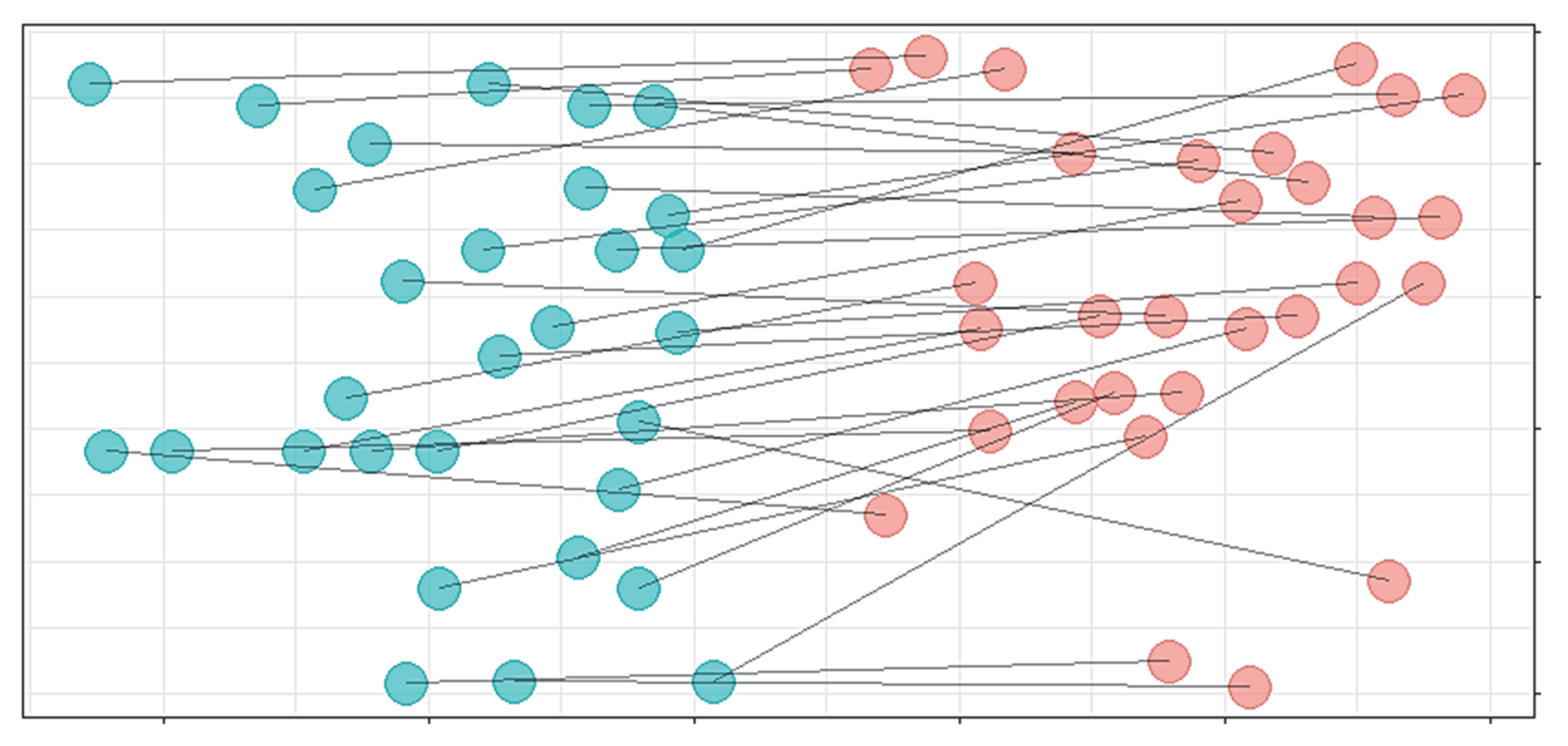
3.1. Homogeneity of Soil Condition Within Sub-Plots

The analysis of soil homogeneity across the study area indicated that the observed characteristics were consistent throughout the permanent study plot. The results of the analysis of variance (ANOVA), including the interaction between the factors “Sub-plot” and “Layer,” revealed no statistically significant differences between sub-plots (p > 0.05, Table 3), suggesting uniform soil conditions within the study area.

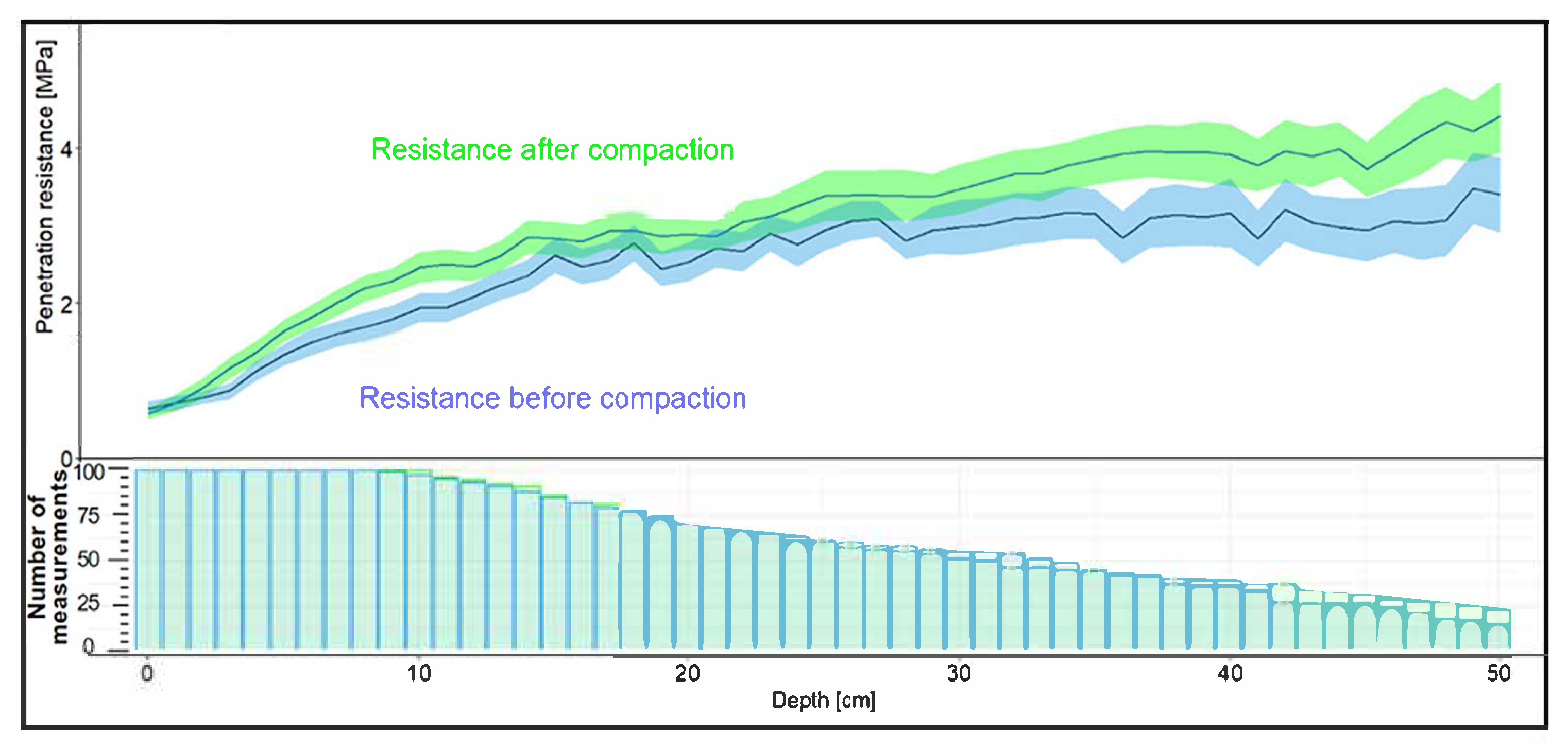
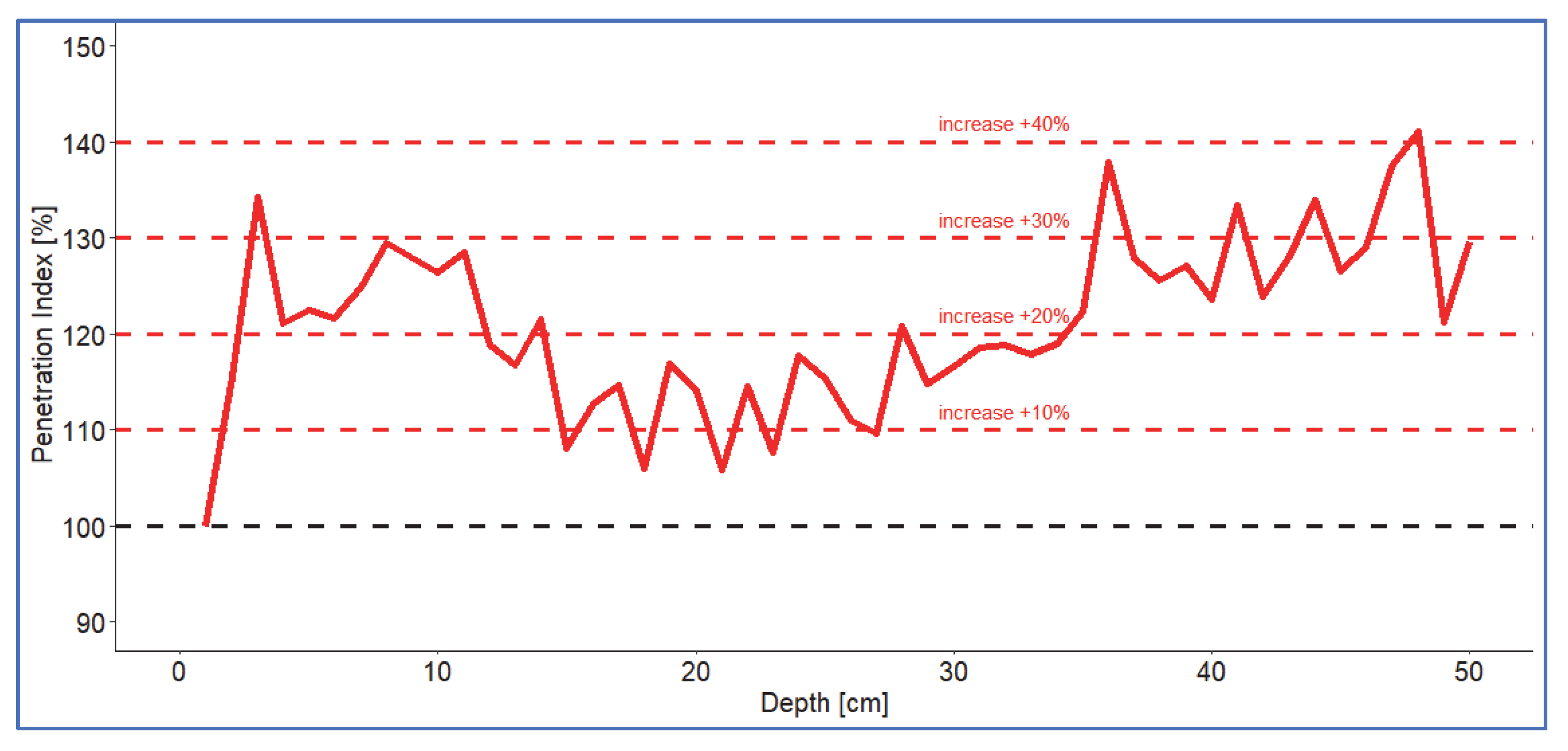
3.2. Penetration Resistance

The variation in penetration resistance, represented as the average value across penetration points with the increasing soil depth at the compacted sub-plot, is presented in Figure 4. The results indicated a notable increase in penetration resistance following soil compaction, with resistance rising throughout the soil profile.
The increase in PR within the compacted sub-plot was quantified by the penetration index, as depicted by the red curve in Figure 5. The average value of the penetration index for soil up to a depth of 10 cm was 119%, reflecting a 19% increase in penetration resistance caused by the skidder passage. In the topsoil, the maximum penetration index was observed at a depth of 3 cm, reaching 134%. Beyond a depth of approximately 15 cm, the penetration index began to decline; however, the difference in penetration resistance showed another upward trend at a depth of around 35 cm, continuing up to 50 cm.

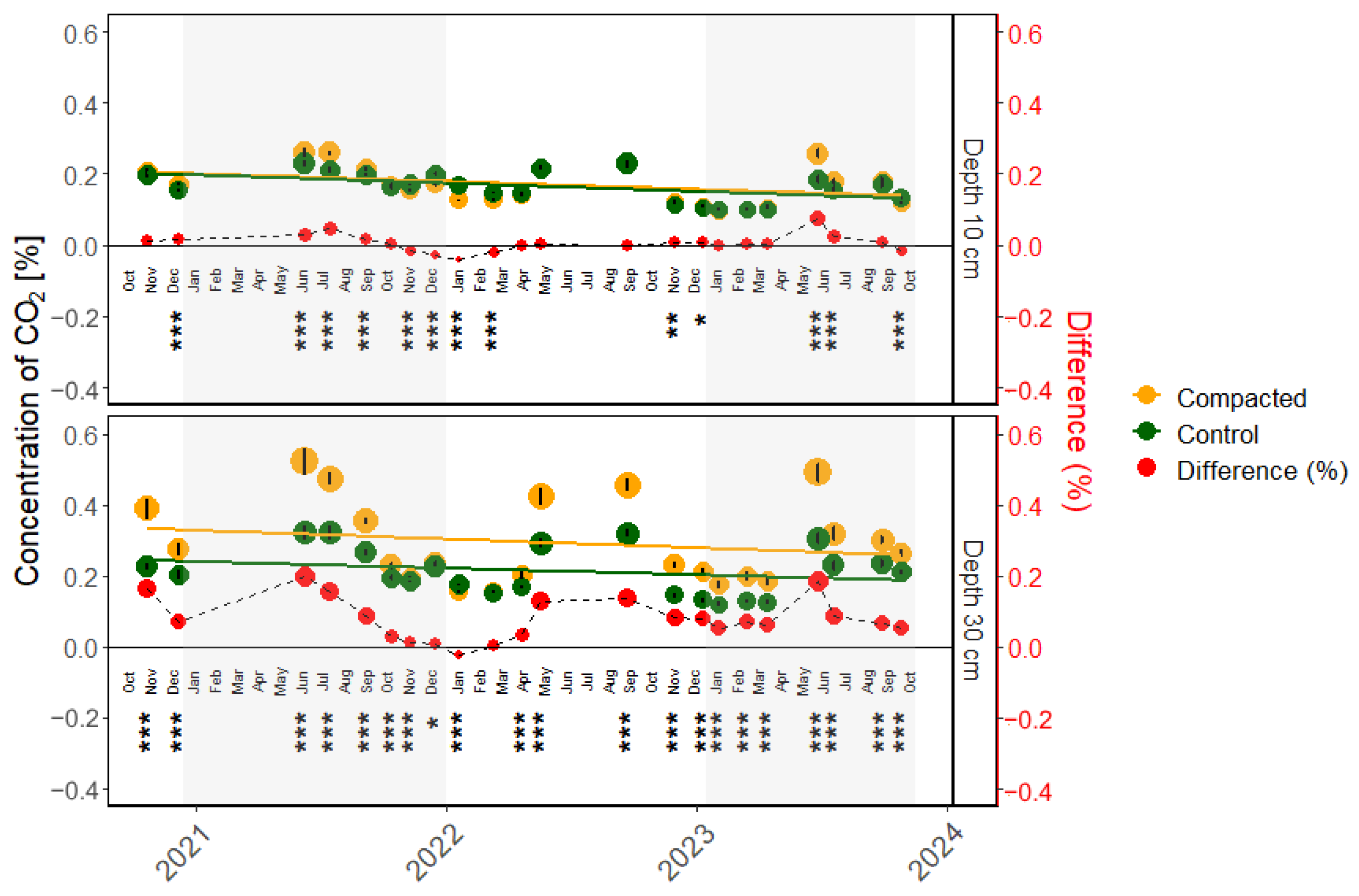
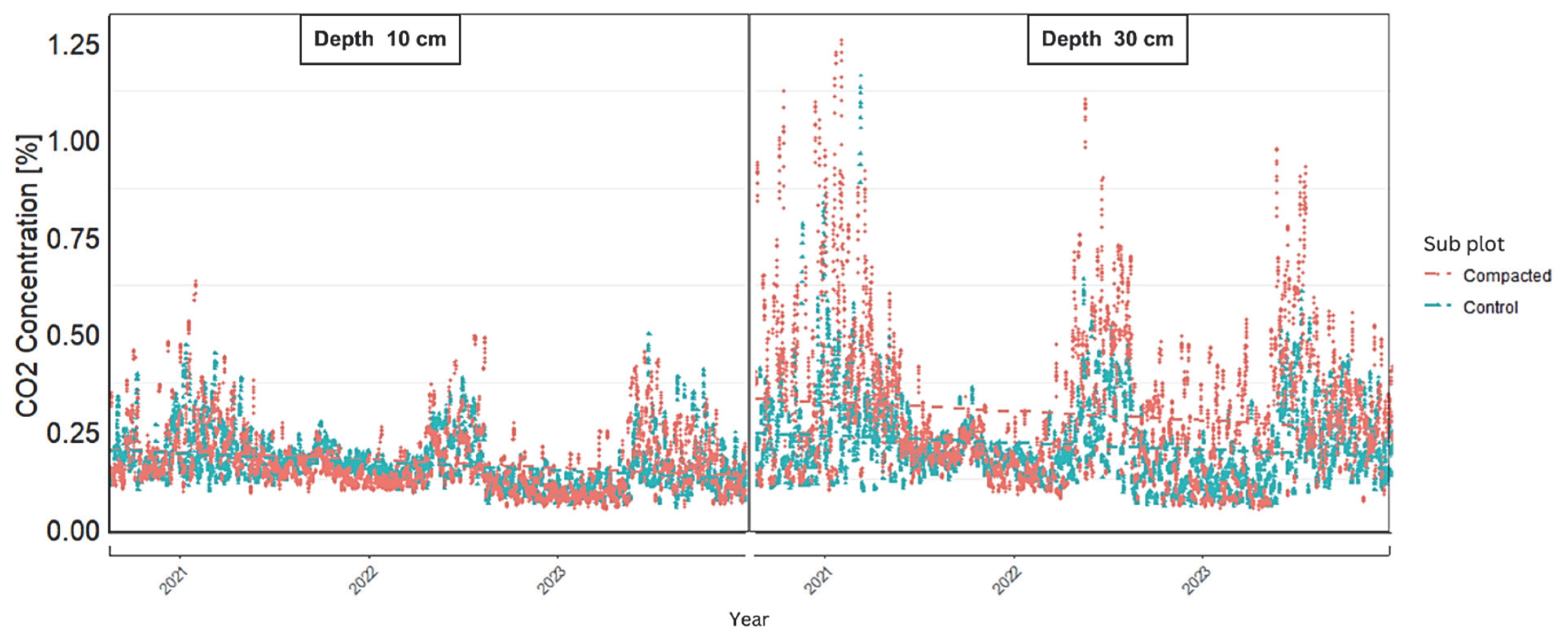
3.3. Concentration of CO2 in the Soil

Soil temperature and soil moisture, as the primary abiotic factors influencing CO2 concentration in soil, contributed to a noticeable seasonal trend, particularly at the compacted sub-plot. Higher CO2 concentrations were recorded during the growing season, while both the variability and concentration of CO2 reached their lowest levels during the winter months. The differences between sub-plots were less pronounced in the winter compared to the growing season (Figure 6).
Statistical analysis revealed significant differences in CO2 concentration at 30 cm depth between the two sub-plots in most months (p < 0.001), with the exception of March 2022, when no significant difference between the sub-plots was detected. In December 2021, the difference was statistically significant at a lower threshold (p < 0.05). At a depth of 10 cm (as shown in the upper part of Figure 6), the differences between the control and compacted sub-plots were less pronounced. During the first year after compaction, the compacted sub-plot exhibited higher CO2 concentrations. However, this trend reversed during the following year, with the control plot showing higher CO2 concentrations from autumn 2021 until early summer 2022. In April 2022, the concentrations began to equalize between the plots, a trend that persisted until the onset of the 2023 growing season. In instances where statistically significant differences between means were observed (p < 0.001), the compacted sub-plot typically exhibited lower CO2 concentrations at a depth of 10 cm, particularly during the months of November 2021, December 2021, January 2022, and March 2022. Conversely, statistically higher CO2 concentrations at a depth of 10 cm at the compacted sub-plot were primarily observed in the early months following compaction (November 2020, December 2020, June 2020, July 2020, and September 2020). Beyond this period, differences either diminished or reversed, as previously noted. After 18 months following compaction, the differences at a depth of 10 cm were minimal and statistically insignificant. This suggests that within two years after the forestry machine’s passage, the CO2 concentration at 10 cm depth returned to levels comparable to those of the control sub-plot, indicating the soil recovery at the compacted sub-plot.
Figure 7 illustrates the variability observed at individual measurement points, depths, and sub-plots over time. CO2 accumulation was primarily observed during the growing season. At the compacted sub-plot, CO2 concentration at a depth of 30 cm ranged from 0.049% to 1.250%, with an average value of 0.281%, while at a depth of 10 cm, the concentration ranged from 0.048% to 0.637%, with an average of 0.165%. At the control sub-plot, CO2 concentration at a depth of 30 cm varied between 0.054% and 1.160%, with an average value of 0.206%. At 10 cm depth, the values ranged from 0.057% to 0.470%, with an average of 0.163%. Over the measurement period from October 2020 to October 2023, a slight decline in CO2 concentration was observed at both plots and both soil depths. Notably, higher CO2 concentrations were recorded at a depth of 30 cm at both compacted and control plots.
The results indicate that CO2 concentration at a soil depth of 10 cm was lower than at 30 cm, although a seasonal trend was still evident at both depths. Figure 8 illustrated the positive correlation between CO2 concentration at 30 cm and relative moisture at both 30 cm and 10 cm (r = 0.7 for each).The weak correlation (r = 0.1) between CO2 concentrations at 30 cm and 10 cm depths suggests that gas dynamics in the upper and lower soil layers were influenced by different factors, which can explain the relatively small transfer of CO2 between these depths. Greater differences between sub-plots were observed at 30 cm depth.
The STL decomposition of soil CO2 concentrations revealed a distinct seasonal trend—seasonal component (Figure 9). The seasonal component exhibited pronounced peaks in CO2 concentration during the growing season, whereas the winter months were characterized by lower CO2 levels and reduced variability. The trend component demonstrated a consistent decline in CO2 concentration over a three-year period following compaction, as illustrated by the trend line.
During the temperature measurements (Figure 10), the control sub-plot consistently exhibited higher soil temperatures. Over the 3-year period, the average temperature at the control sub-plot was 0.20 °C (+3%) higher at 10 cm depth and 0.21 °C (+3%) higher at 30 cm depth. The most pronounced temperature differences occurred in spring, at the onset of the growing season, with the largest discrepancy at 10 cm (+0.61 °C) recorded on 13 April 2023 and at 30 cm (+0.76 °C) on 21 April 2022. Seasonal analyses revealed that mean temperature differences at 10 cm between the control and the compacted sub-plot were +0.45 °C in spring (March, April, and May), +0.14 °C in summer (June, July, and August), +0.14 °C in autumn (September, October, and November), and +0.03 °C in winter (December, January, and February). At 30 cm, the differences were +0.46 °C in spring, +0.18 °C in summer, +0.12 °C in autumn, and +0.03 °C in winter. These temperature differences between sub-plots were statistically significant (p < 0.05), except on 1 February 2023. Temperature variability was found to be highest in autumn and spring, with SD (standard deviation) values ranging from 3.5 to 3.7 °C at both depths. These increased fluctuations can be attributed to transient seasonal conditions when changes between cooler and warmer temperatures are more frequent. Conversely, winter and summer showed the lowest temperature variability (1.3–1.9 °C), indicating greater temperature stability during these periods of more stable atmospheric conditions.
Soil moisture measurements (Figure 11) showed greater differences between sub-plots than those observed for soil temperature, with the most substantial differences occurring in winter and spring. At the control sub-plot, soil moisture was on average −7.77% (−15%) lower at 10 cm depth and −7.92% (−16%) lower at 30 cm depth than at the compacted soil. The greatest differences in soil moisture at 10 and 30 cm soil depth of −25.20% and −25.45%, respectively, were recorded on 1 February 2023. Seasonal comparisons of soil moisture revealed differences at 10 cm depth of −7.06% in spring, −5.60% in summer, −5.00% in autumn, and −8.98% in winter. At 30 cm, the differences were −11.29% in spring, −6.34% in summer, −5.99% in autumn, and −10.6% in winter.

4. Discussion

Our study demonstrated that tractor traffic caused significant changes in soil physical properties, particularly in the form of increased compaction. This mechanical disturbance led to changes in soil gas exchange dynamics, soil temperature, and moisture regime. A partial recovery of CO2 levels was observed at 10 cm depth over the two years, but this recovery was not evident at greater depths. At 30 cm depth, there was a statistically significant difference in CO2 concentration between the control and compacted sub-plots throughout the measurement period.

4.1. Soil Compaction

This study revealed significantly increased values of penetration resistance, as indicated by the penetration index. Following the compaction treatment, penetration resistance values were elevated by an average of 19% at the 0–10 cm soil depth, reaching the maximum increase of 34% at the 3 cm depth. These findings align with broader evidence that mechanized operations influence surface and soil structure [7,11,18,23], thereby influencing penetration resistance [24]. However, Kormanek et al. [25] reported a limited impact of machine traffic. This contrast may be attributed to the protective effect of the surface organic layer and the use of low ground-pressure machinery [9,26]. The increase in penetration resistance was strongly correlated with elevated CO2 concentrations at the depth of 30 cm (r = 0.8), suggesting that reduced soil porosity—resulting from compaction—limited gas diffusion and contributed to CO2 accumulation in deeper soil layers. These findings align with Feng et al. [4], who reported that compaction reduces soil gas permeability by 63%–93%. Similar conclusions were reached by Kim et al. [14], who observed significant increases in soil CO2 concentrations in compacted soils, especially during the growing season.

4.2. Soil CO2 Concentrations

Over the three-year period following the compaction treatment, average soil CO2 concentrations were consistently and significantly higher in the compacted sub-plot compared to the control. At a depth of 30 cm, 21 out of 22 measurements showed statistically significant differences (p < 0.05), while at a depth of 10 cm, significant differences were observed in 13 out of 22 measurements. (p < 0.05). The average CO2 concentration in the compacted sub-plot was 0.293% at a depth of 30 cm and 0.169% at 10 cm. In comparison, the control sub-plot recorded average concentrations of 0.214% at 30 cm and 0.163% at 10 cm. These results also confirm that CO2 concentrations were generally higher at greater soil depths and are consistent with findings from previous studies, which have shown that CO2 concentrations tend to increase with depth due to reduced diffusion rates, greater microbial activity, and root respiration in deeper soil layers [12,27]. Moreover, it has been reported that CO2 concentrations in the organic horizon are typically only slightly above atmospheric levels (e.g., around 0.04%), whereas concentrations increase significantly in the mineral layers below [3,28]. The analysis of our data clearly showed that soil CO2 concentrations increased with compaction treatment. Allman et al. [29] reported that forestry machine traffic significantly affects CO2 concentration in soils. Critical concentration of CO2 fluctuates around 0.6%, and exceeding this threshold can result in reduced root growth in seedlings [30,31,32]. In our study, the mean CO2 concentrations in compacted sub-plots remained well below this critical threshold across all years and depths. At 30 cm depth, average concentrations in the compacted sub-plot declined from 0.348% in the first year post-compaction to 0.265% and 0.267% in the second and third years, respectively. Similarly, at 10 cm depth, values decreased from 0.203% to 0.143% over the same period. Although compaction clearly elevated CO2 levels relative to control sub-plots—where mean concentrations ranged from 0.246% to 0.186% at 30 cm and from 0.188% to 0.130% at 10 cm—these levels remained below the 0.6% threshold associated with physiological stress in plant roots. These findings suggest that while compaction can significantly affect gas dynamics in forest soils, the observed concentrations may not reach levels considered critical for root function, particularly in the context of moderately compacted soils.

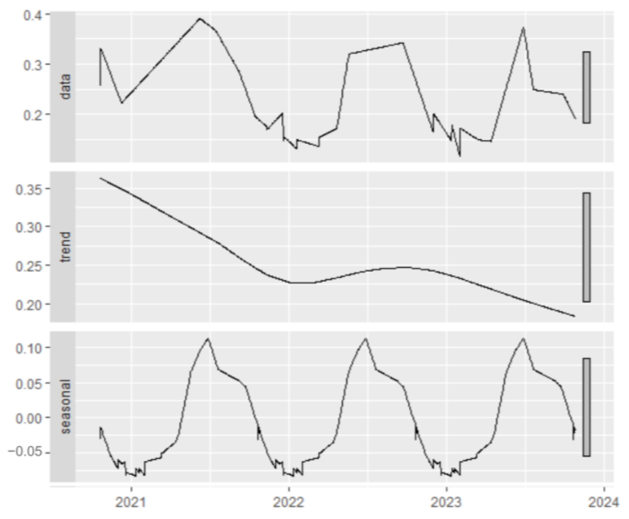
4.3. Seasonal Trend in CO2 Concentrations

A distinct seasonal pattern in soil CO2 concentration was observed, with higher values at 30 cm depth during the growing season (April to September) and lower, less variable concentrations in winter (December to February). Sub-plot differences were more pronounced during the growing season and diminished in winter. STL decomposition further confirmed this seasonal trend, showing clear peaks during the growing season and a consistent decline in CO2 concentration over the three years post-compaction, as indicated by the trend component (Figure 9). Similar seasonal trends have been documented in other studies. For instance, studies in European beech and Scots pine stands reported CO2 concentration minima in winter and peaks in summer, closely associated with changes in soil temperature and moisture [33]. In a Finnish Scots pine forest, soil CO2 efflux varied seasonally, with higher rates in late summer compared to spring at equivalent soil temperatures, indicating the influence of biological activity such as root and microbial respiration [34]. Consistent with prior findings [3], our data showed lower CO2 concentrations at 10 cm compared to 30 cm depth, with both depths exhibiting seasonal fluctuations. Kim et al. [14] also reported higher soil CO2 concentrations primarily during the growing season, with reduced variability and negligible differences during winter. Similarly, the highest concentrations were typically observed in late summer (August–September), while the lowest occurred in winter (December–February) [1].

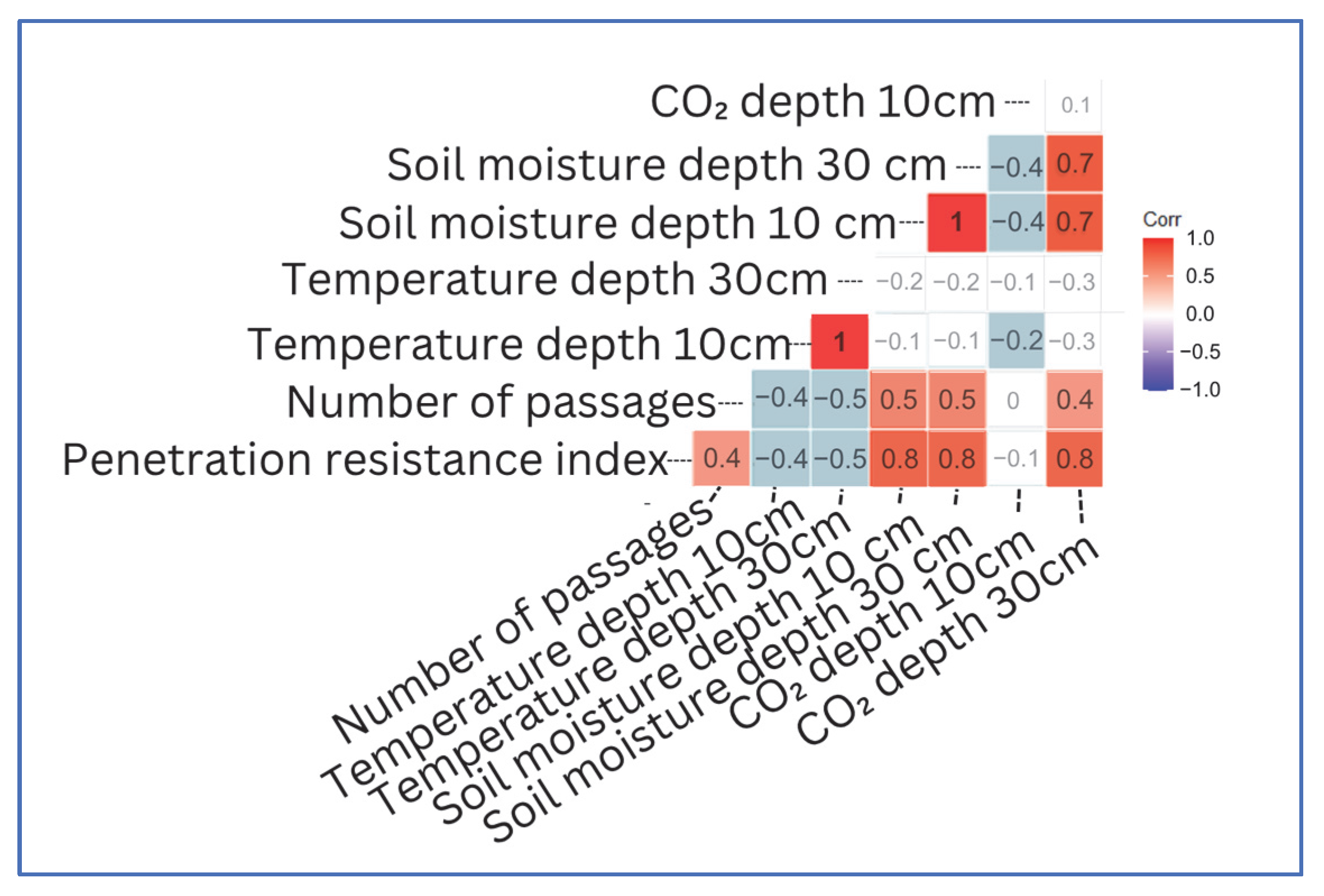
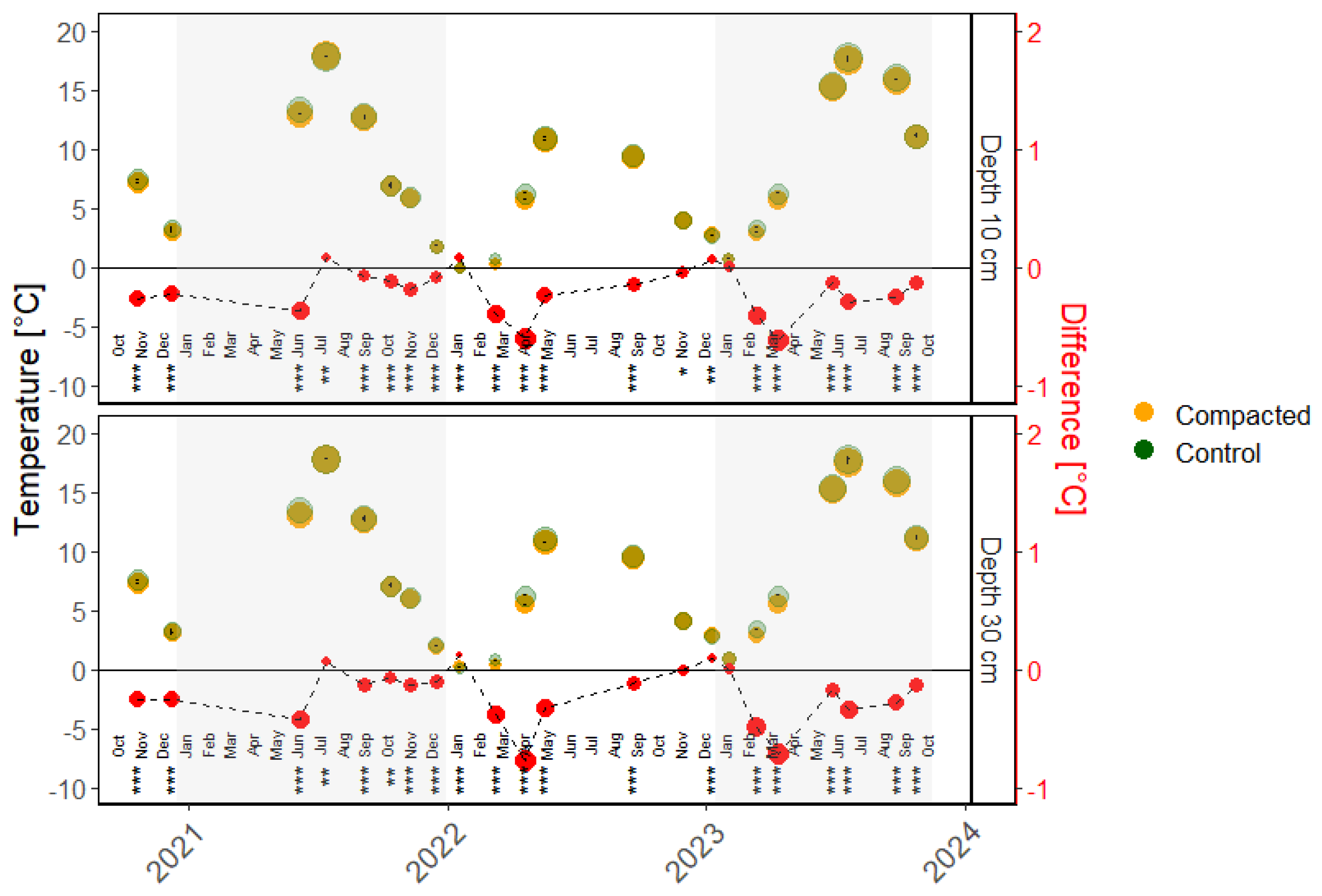
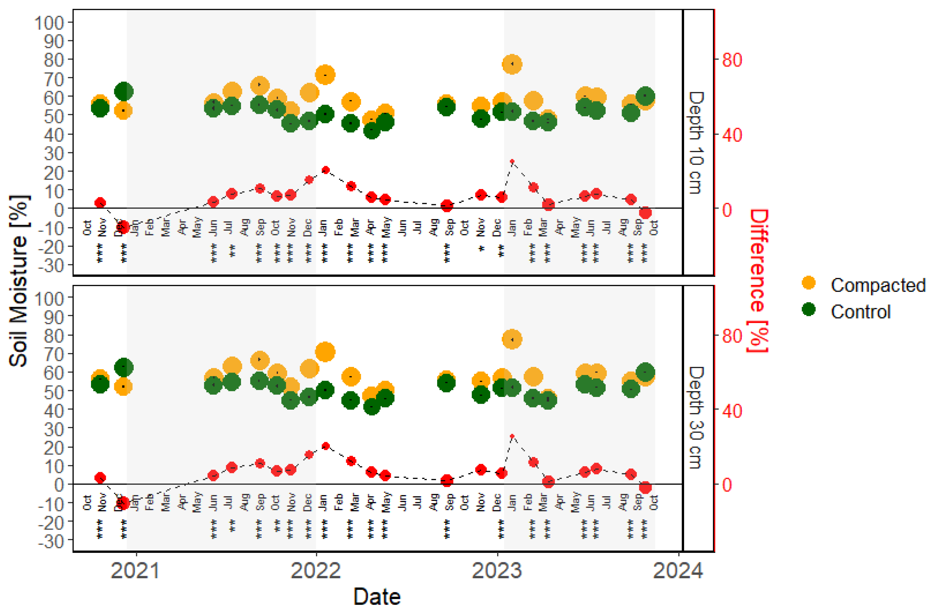
4.4. Temperature and Soil Moisture Regimes

Soil moisture measurements revealed pronounced differences between compacted and control sub-plots, particularly during winter and spring, with the most substantial deviation recorded on 1 February 2023—25.2% at 10 cm and 25.45% at 30 cm depth (Figure 11). On average, soil moisture at the control sub-plot was 7.77% lower at 10 cm and 7.92% lower at 30 cm compared to the compacted sub-plot, with seasonal contrasts most evident in spring and winter. Higher soil moisture in the compacted sub-plot suggests slower water infiltration and reduced hydraulic conductivity, likely due to compaction, which also affects the soil’s water regime and temperature. The increased soil moisture on the compacted sub-plot contributes to lower soil temperatures, likely due to reduced permeability of the upper soil layers and increased water retention. The results of another study show that compaction slows water percolation by reducing soil pore space, potentially leading to surface runoff [35]. However, given that the study area is situated on a gentle slope (<5%), surface runoff is unlikely. Instead, the elevated moisture content is more plausibly attributed to localized waterlogging caused by restricted drainage in compacted soils. Soil compaction during mechanized logging reduces macropores in the soil [36], thereby decreasing water infiltration [37] and increasing the potential for soil erosion on steeper slopes [38]. On flat or mildly sloped areas, compaction leads to slower water infiltration and waterlogging [39]. In our study, reduced soil porosity and infiltration in the compacted sub-plot led to an average increase of 15% in soil moisture, likely due to enhanced surface water retention and slower drainage. The maximum observed difference of +25% on 1 February 2023 indicates the potential for prolonged waterlogging or inefficient water redistribution in the compacted areas. With an increasing number of machinery passes, the infiltration rate further declines. The most significant change occurs after the initial passes, when the infiltration rate can drop by up to 50% [37]. A moderate positive correlation (r = 0.5) between soil moisture and the number of machine passages, along with a strong positive correlation (r = 0.8) between soil moisture and the penetration resistance index—a proxy for soil compaction—suggests that compaction increased soil moisture content by reducing soil permeability and impeding water infiltration. Barik et al. [40] obtained similar results in their study, where they measured soil moisture content up to a depth of 30 cm. After compaction, soil moisture increased on average by 12.7%. Significant differences in soil moisture following compaction were also reported in other studies [41,42,43]. Hydraulic conductivity is a highly sensitive indicator of soil compaction. Compared to bulk density and reduced soil porosity, hydraulic conductivity exhibited the most significant change in 67 studies focusing on soil compaction and its effects on soil characteristics [23]. The primary cause of the large reduction in hydraulic conductivity is the decrease in macropores, which play a critical role in water infiltration into the soil [44].

4.5. Recovery of Soil

In our study, even two years after the passage of forestry machinery, higher CO2 concentrations were measured at a depth of 30 cm. Unlike the 10 cm depth, where CO2 concentration in the compacted sub-plot stabilized at levels comparable to the control sub-plot, the CO2 concentration at 30 cm depth at the compacted sub-plot did not reach the control level even after two years. However, we observed a declining trend in CO2 concentration at this depth, indicating a possible recovery (Figure 9). Further long-term monitoring is necessary to estimate the timeline for soil recovery after compaction, particularly in deeper soil horizons. The recovery time of soil following compaction can vary widely, from as short as one year [15] to as long as 20 years [16], depending on the parameter used to assess the recovery and also on soil characteristics [17], environmental conditions [18], and duration and intensity of machinery impact [45,46]. According to Labelle [47], soil recovery can take between 5 and 30 years.

5. Conclusions

This study highlights the significant impact of forest machinery operation on soil compaction and the associated effects on soil properties and CO2 dynamics. The results confirmed that soil compaction increased penetration resistance, with values increasing on average by 19% (0–10 cm depth) and reaching a maximum of 34% (3 cm depth).
Our findings show that CO2 concentrations in compacted soils remained elevated two years after machinery passage, especially in deeper layers. At a depth of 10 cm, CO2 concentrations reached the levels comparable to the control plot within two years, indicating partial recovery in the topsoil. However, deeper layers showed slower recovery, with CO2 levels at 30 cm still significantly higher at the compacted sub-plot. Seasonal variability in CO2 concentration was also evident, with the highest values observed during the growing season due to reduced permeability in the compacted soil layer and increased autotrophic respiration by root systems and rhizosphere microorganisms.
These results are consistent with previous studies showing that soil compaction reduces hydraulic conductivity, air permeability, and porosity, thereby limiting gas exchange and water infiltration while increasing moisture retention. The reduced permeability of compacted soils creates conditions that inhibit the diffusion of CO2 and lead to its accumulation beneath the compacted layer. This phenomenon is exacerbated during the growing season when biological activity peaks, while differences between sub-plots are less pronounced during winter months.
Considering these findings, forest management should prioritize minimizing soil compaction to protect soil structure and function. The most effective mitigation strategy involves restricting forest machinery movements to designated skid trails and avoiding uncontrolled traffic through forest stands. Long-term monitoring is essential to better understand the timing of restoration of deeper soil horizons and to develop sustainable silvicultural practices that maintain soil health and ecosystem function. Thanks to the three-year duration of the experiment, we were able to investigate the dynamics of soil characteristics, including temperature, moisture, and CO2 concentration, as well as their temporal development following the soil compaction event.

Author Contributions

Conceptualization, D.T. and J.M.; methodology, D.T., J.M., M.A., M.F., V.J., and M.V.; software, D.T.; validation, D.T., J.M., and K.M.; formal analysis, D.T., K.M., and J.V.; investigation, D.T., J.M., M.A., M.F., and Z.D.; resources, J.M.; data curation, D.T., J.M., and K.M.; writing—original draft preparation, D.T. and J.M.; writing—review and editing, D.T., J.M., and K.M.; visualization, D.T.; supervision, J.M. and K.M.; project administration, J.M.; funding acquisition, D.T., J.M., and M.F. All authors have read and agreed to the published version of the manuscript.

Funding

This research was funded by EU NextGenerationEU through the Recovery and Resilience Plan for Slovakia, grant numbers 09I03-03-V05-00016 and 09I03-03-V04-00130; by the Slovak Research and Development Agency, grant numbers APVV-22-0001, APVV-21-0412, APVV-18-0305, and VV-MVP-24-0412; by the Scientific Grant Agency VEGA, grant numbers VEGA 1/0177/24 and VEGA 1/0604/24; and Cultural and Education Grant Agency Ministry of Education, Research Development, and Youth of the Slovak Republic, grant number KEGA 004TU Z-4/2023.

Data Availability Statement

The original contributions presented in this study are included in the article. Further inquiries can be directed to the corresponding author.

Acknowledgments

During the preparation of this manuscript, the author(s) used ChatGPT-3.5 Mini to improve grammar. The authors have reviewed and edited the output and take full responsibility for the content of this publication.

Conflicts of Interest

The authors declare no conflicts of interest.

References

  1. Huang, F.; Cao, J.; Zhu, T.; Fan, M.; Ren, M. CO2 Transfer Characteristics of Calcareous Humid Subtropical Forest Soils and Associated Contributions to Carbon Source and Sink in Guilin, Southwest China. Forests 2020, 11, 219. [Google Scholar] [CrossRef]
  2. Munjonji, L.; Ayisi, K.K.; Mafeo, T.P.; Maphanga, T.; Mabitsela, K.E. Seasonal Variation in Soil CO2 Emission and Leaf Gas Exchange of Well-managed Commercial Citrus sinensis (L.) Orchards. Plant Soil 2021, 465, 65–81. [Google Scholar] [CrossRef]
  3. Conlin, T.S.S.; Driessche, R. van den Response of Soil CO2 and O2 Concentrations to Forest Soil Compaction at the Long-Term Soil Productivity Sites in Central British Columbia. Can. J. Soil. Sci. 2000, 80, 625–632. [Google Scholar] [CrossRef]
  4. Feng, L.; Hu, J.; Jiang, J. Uncertainty in Soil Gas Permeability Measurements. Front. Environ. Sci. 2025, 13, 1474764. [Google Scholar] [CrossRef]
  5. Poungparn, S.; Komiyama, A.; Tanaka, A.; Sangtiean, T.; Maknual, C.; Kato, S.; Tanapermpool, P.; Patanaponpaiboon, P. Carbon Dioxide Emission Through Soil Respiration in a Secondary Mangrove Forest of Eastern Thailand. J. Trop. Ecol. 2009, 25, 393–400. [Google Scholar] [CrossRef]
  6. Allman, M.; Allmanová, Z.; Jankovský, M.; Ferenčík, M.; Messingerová, V. Damage of the Remaining Stands Caused by Various Types of Logging Technology. Acta Univ. Agric. Silvic. Mendel. Brun. 2016, 64, 379–385. [Google Scholar] [CrossRef]
  7. Allman, M.; Jankovský, M.; Messingerová, V.; Allmanová, Z.; Ferenčík, M. Soil Compaction of Various Central European Forest Soils Caused by Traffic of Forestry Machines with Various Chassis. For. Syst. 2015, 24, e038. [Google Scholar] [CrossRef]
  8. Agherkakli, B.; Najafi, A.; Sadeghi, S.H. Ground Based Operation Effects on Soil Disturbance by Steel Tracked Skidder in a Steep Slope of Forest. J. For. Sci. 2010, 56, 278–284. [Google Scholar] [CrossRef]
  9. Ring, E.; Andersson, M.; Hansson, L.; Jansson, G.; Högbom, L. Logging Mats and Logging Residue as Ground Protection during Forwarder Traffic along Till Hillslopes. Croat. J. For. Eng. 2021, 42, 445–462. [Google Scholar] [CrossRef]
  10. Warlo, H.; Von Wilpert, K.; Lang, F.; Schack-Kirchner, H. Black Alder (Alnus glutinosa (L.) Gaertn.) on Compacted Skid Trails: A Trade-off between Greenhouse Gas Fluxes and Soil Structure Recovery? Forests 2019, 10, 726. [Google Scholar] [CrossRef]
  11. Eliasson, L. Effects of Forwarder Tyre Pressure on Rut Formation and Soil Compaction. Silva Fenn. 2005, 39, 366. [Google Scholar] [CrossRef]
  12. Davidson, E.A.; Savage, K.E.; Trumbore, S.E.; Borken, W. Vertical Partitioning of CO2 Production within a Temperate Forest Soil. Glob. Change Biol. 2006, 12, 944–956. [Google Scholar] [CrossRef]
  13. Yamulki, S.; Forster, J.; Xenakis, G.; Ash, A.; Brunt, J.; Perks, M.; Morison, J.I.L. Effects of Clear-Fell Harvesting on Soil CO2, CH4, and N2O Fluxes in an Upland Sitka Spruce Stand in England. Biogeosciences 2021, 18, 4227–4241. [Google Scholar] [CrossRef]
  14. Kim, I.; Han, S.-K.; Acuna, M.; Woo, H.; Oh, J.-H.; Choi, B. Effect of Heavy Machine Traffic on Soil CO2 Concentration and Efflux in a Pinus Koraiensis Thinning Stand. Forests 2021, 12, 1497. [Google Scholar] [CrossRef]
  15. Mace, A.C. Recovery of forest soils from compaction by rubber-tired skidders. Minn. For. Res. Notes 1971, 4, 226. [Google Scholar]
  16. Jakobsen, B.F.; Greacen, E.L. Compaction of Sandy Forest Soils by Forwarder Operations. Soil Tillage Res. 1985, 5, 55–70. [Google Scholar] [CrossRef]
  17. Cambi, M.; Grigolato, S.; Neri, F.; Picchio, R.; Marchi, E. Effects of Forwarder Operation on Soil Physical Characteristics: A Case Study in the Italian Alps. Croat. J. For. Eng. 2016, 37, 233–239. [Google Scholar]
  18. Ampoorter, E.; de Schrijver, A.; van Nevel, L.; Hermy, M.; Verheyen, K. Impact of Mechanized Harvesting on Compaction of Sandy and Clayey Forest Soils: Results of a Meta-Analysis. Ann. For. Sci. 2012, 69, 533–542. [Google Scholar] [CrossRef]
  19. Slovenský Hydrometeorologický Ústav. Klimatický Atlas Slovenska; Slovenský Hydrometeorologický Ústav: Bratislava, Slovakia, 2015; 132p, ISBN 97880-88907-90-9. [Google Scholar]
  20. National Forest Centre. Forestry Information System 2023–2032; National Forest Centre: Zvolen, Slovakia, 2023.
  21. QGIS Development Team. QGIS Geographic Information System, Version 3.14; Open Source Geospatial Foundation: Beaverton, OR, USA, 2020. [Google Scholar]
  22. RStudio Team. R: A Language and Environment for Statistical Computing; R Foundation for Statistical Computing: Vienna, Austria, 2024; Available online: https://www.r-project.org/ (accessed on 10 October 2024).
  23. Nazari, M.; Eteghadipour, M.; Zarebanadkouki, M.; Ghorbani, M.; Dippold, M.A.; Bilyera, N.; Zamanian, K. Impacts of Logging-Associated Compaction on Forest Soils: A Meta-Analysis. Front. For. Glob. Change 2021, 4, 780074. [Google Scholar] [CrossRef]
  24. Benevenute, P.A.N.; de Morais, E.G.; Souza, A.A.; Vasques, I.C.F.; Cardoso, D.P.; Sales, F.R.; Severiano, E.C.; Homem, B.G.C.; Casagrande, D.R.; Silva, B.M. Penetration Resistance: An Effective Indicator for Monitoring Soil Compaction in Pastures. Ecol. Indic. 2020, 117, 106647. [Google Scholar] [CrossRef]
  25. Kormanek, M.; Dvořák, J.; Tylek, P.; Jankovský, M.; Nuhlíček, O.; Mateusiak, Ł. Impact of MHT9002HV Tracked Harvester on Forest Soil after Logging in Steeply Sloping Terrain. Forests 2023, 14, 977. [Google Scholar] [CrossRef]
  26. Ilintsev, A.; Nakvasina, E.; Högbom, L. Methods of Protection Forest Soils during Logging Operations (Review). Lesn. Zhurnal 2021, 2021, 92–116. [Google Scholar] [CrossRef]
  27. Högberg, P.; Nordgren, A.; Buchmann, N.; Taylor, A.F.S.; Ekblad, A.; Högberg, M.N.; Nyberg, G.; Ottosson-Löfvenius, M.; Read, D.J. Large-Scale Forest Girdling Shows That Current Photosynthesis Drives Soil Respiration. Nature 2001, 411, 789–792. [Google Scholar] [CrossRef] [PubMed]
  28. Subke, J.-A.; Bahn, M. On the “Temperature Sensitivity” of Soil Respiration: Can We Use the Immeasurable to Predict the Unknown? Soil Biol. Biochem. 2010, 42, 1653–1656. [Google Scholar] [CrossRef]
  29. Allman, M.; Jankovský, M.; Messingerová, V.; Allmanová, Z. Changes of Carbon Dioxide Concentration in Soils Caused by Forestry Machine Traffic. For. J. 2016, 62, 23–28. [Google Scholar] [CrossRef]
  30. Cambi, M.; Hoshika, Y.; Mariotti, B.; Paoletti, E.; Picchio, R.; Venanzi, R.; Marchi, E. Compaction by a Forest Machine Affects Soil Quality and Quercus robur L. Seedling Performance in an Experimental Field. For. Ecol. Manag. 2017, 384, 406–414. [Google Scholar] [CrossRef]
  31. Gebauer, R.; Martinková, M. Effects of Pressure on the Root Systems of Norway Spruce Plants (Picea abies [L.] Karst.). J. For. Sci. 2012, 51, 268–275. [Google Scholar] [CrossRef]
  32. Jourgholami, M. Effects of Soil Compaction on Growth Variables in Cappadocian Maple (Acer cappadocicum) Seedlings. J. For. Res. 2018, 29, 601–610. [Google Scholar] [CrossRef]
  33. Jochheim, H.; Wirth, S.; Gartiser, V.; Paulus, S.; Haas, C.; Gerke, H.H.; Maier, M. Dynamics of Soil CO2 Efflux and Vertical CO2 Production in a European Beech and a Scots Pine Forest. Front. For. Glob. Change 2022, 5, 826298. [Google Scholar] [CrossRef]
  34. Niinistö, S.M.; Kellomäki, S.; Silvola, J. Seasonality in a Boreal Forest Ecosystem Affects the Use of Soil Temperature and Moisture as Predictors of Soil CO2 Efflux. Biogeosciences 2011, 8, 3169–3186. [Google Scholar] [CrossRef]
  35. Gregory, J.H.; Dukes, M.D.; Jones, P.H.; Miller, G.L. Effect of Urban Soil Compaction on Infiltration Rate. J. Soil Water Conserv. 2006, 61, 117–124. [Google Scholar] [CrossRef]
  36. Carter, M.R. Relationship of Strength Properties to Bulk Density and Macroporosity in Cultivated Loamy Sand to Loam Soils. Soil Tillage Res. 1990, 15, 257–268. [Google Scholar] [CrossRef]
  37. Startsev, A.D.; McNabb, D.H. Effects of Skidding on Forest Soil Infiltration in West-Central Alberta. Can. J. Soil. Sci. 2000, 80, 617–624. [Google Scholar] [CrossRef]
  38. Vaezi, A.R.; Ahmadi, M.; Cerdà, A. Contribution of Raindrop Impact to the Change of Soil Physical Properties and Water Erosion under Semi-Arid Rainfalls. Sci. Total Environ. 2017, 583, 382–392. [Google Scholar] [CrossRef]
  39. Parajuli, M.; Hiesl, P.; Hagan, D.; Khanal, P. Logging Operations and Soil Compaction; Land-Grant Press: Clemson, SC, USA, 2022. [Google Scholar]
  40. Barik, K.; Aksakal, E.L.; Islam, K.R.; Sari, S.; Angin, I. Spatial Variability in Soil Compaction Properties Associated with Field Traffic Operations. CATENA 2014, 120, 122–133. [Google Scholar] [CrossRef]
  41. Dauda, A.; Samari, A. Cowpea Yield Response to Soil Compaction under Tractor Traffic on a Sandy Loam Soil in the Semi-Arid Region of Northern Nigeria. Soil Tillage Res. 2002, 68, 17–22. [Google Scholar] [CrossRef]
  42. Mamman, E.; Ohu, J.O. Millet Yield as Affected by Tractor Traffic in a Sandy Loam Soil in Borno State, Nigeria. Soil Tillage Res. 1997, 42, 133–140. [Google Scholar] [CrossRef]
  43. Ohu, J.O.; Gbalapun, A.H.; Folorunso, O.A. The Effect of Tractor Traffic on Cotton Production in Dark Clay Soil [Numan, Adamawa]; Kongelige Veterinaerog Landbohoejskole: Frederiksberg, Denmark, 1994. [Google Scholar]
  44. Ampoorter, E.; Goris, R.; Cornelis, W.M.; Verheyen, K. Impact of Mechanized Logging on Compaction Status of Sandy Forest Soils. For. Ecol. Manag. 2007, 241, 162–174. [Google Scholar] [CrossRef]
  45. Berisso, F.E.; Schjønning, P.; Keller, T.; Lamandé, M.; Etana, A.; De Jonge, L.W.; Iversen, B.V.; Arvidsson, J.; Forkman, J. Persistent Effects of Subsoil Compaction on Pore Size Distribution and Gas Transport in a Loamy Soil. Soil Tillage Res. 2012, 122, 42–51. [Google Scholar] [CrossRef]
  46. Shaheb, M.R.; Venkatesh, R.; Shearer, S.A. A Review on the Effect of Soil Compaction and Its Management for Sustainable Crop Production. J. Biosyst. Eng. 2021, 46, 417–439. [Google Scholar] [CrossRef]
  47. Labelle, E.R. Assessing Soil Disturbances Caused by Forest Machinery. Master’s Thesis, University of New Brunswick, Fredericton, NB, Canada, 2008. [Google Scholar] [CrossRef]
Figure 1. (a) Geographical position of the research plot within Slovakia. (b) Detail of the permanent research plot. (c) Forestry skidder (LKT 81 ITL) used for soil compaction.
Forests 16 01025 g001
Figure 2. Permanent research plot (PRP) Stagiar: control sub-plot (left), compacted sub-plot (right). Red circles—soil sampling locations; blue X—location of penetrometer measurements; and orange lines represent tractor passages.
Forests 16 01025 g002
Figure 3. Pairs of points used for CO2 measurements (green points located at the control sub-plot, red points located at the compacted sub-plot) and sampling design of the measurements within the PRP Stagiar.
Forests 16 01025 g003
Figure 4. The effect of compaction on penetration resistance within a compacted sub-plot. The solid lines through the center of the colored buffer represent the mean values at respective depths, with a 95% confidence interval displayed in color around the mean.
Forests 16 01025 g004
Figure 5. The effect of compaction on penetration resistance represented by the penetration index along the soil profile.
Forests 16 01025 g005
Figure 6. Comparison of mean CO2 concentrations at the control (green) and compacted (orange) sub-plots, including the differences (red) between the sub-plots at depths of 10 cm and 30 cm. The size of each point represents the mean CO2 concentration value, while the black vertical lines within the points represent 95% confidence intervals of the mean that indicate variability of measured values. Significant differences between the sub-plots are indicated as follows: 0.001 ‘***’, 0.01 ‘**’, 0.05 ‘*’.
Forests 16 01025 g006
Figure 7. Variability of CO2 concentration measurements at soil depths of 10 cm and 30 cm across sub-plots, including trend lines (dashed) that indicate the long-term development of the CO2 concentration in soil.
Forests 16 01025 g007
Figure 8. The correlation matrix between key variables. The values represent Spearman’s correlation coefficient (significant correlations indicated by color and non-significant correlations left uncolored).
Forests 16 01025 g008
Figure 9. Seasonal-Trend Decomposition (STL) of CO2 concentrations at the compacted plot using Loess over a three-year period following compaction.
Forests 16 01025 g009
Figure 10. Comparison of mean temperature at the control (green) and compacted (orange) sub-plot, including the differences (red) at depths of 10 cm and 30 cm. The size of each point represents the temperature value, while the black vertical lines within points represent 95% confidence intervals of the mean and indicate measurement variability. Significant differences between the sub-plots are indicated as follows: 0.001 ‘***’, 0.01 ‘**’, 0.05 ‘*’.
Forests 16 01025 g010
Figure 11. Comparison of mean soil moisture at the control (green) and compacted (orange) sub-plots, including the differences (red) at depths of 10 cm and 30 cm. The size of each point represents the soil moisture, while the black vertical lines within points represent 95% confidence intervals of the mean and indicate measurement variability. Significant differences between the sub-plots are indicated as follows: 0.001 ‘***’, 0.01 ‘**’, 0.05 ‘*’.
Forests 16 01025 g011
Table 1. Basic stand and site characteristics and soil parameters [20].
Stand Characteristic
Stand No. 554
Age (years): 95
Area of stand (ha) 5.82
Stocking degree0.87
Slope (%)20
AspectWest
Management system Shelterwood
Altitude (m a. s. l.)710
Tree species composition (%) Fagus sylvatica L. (73); Abies alba Mill. (24), Picea abies (L.) H. Karst. (3)
Skidding distance (m)50
Soil typeCambisol
Soil textureSilt Clay
Site Characteristic
Tree species composition (%)Fagus sylvatica L. (95); Abies alba Mill. (5)
Slope0%–5%
Loam content (<0.002 mm) (%)4.5
Silt content (0.002–0.063 mm) (%)69.13
Sand content (0.063–2 mm) (%)26.82
Table 2. Technical parameters of the forestry skidder LKT 81 ITL.
EngineHydraulic ManipulatorMachine Width (cm)Front/Rear Tires (inch)Tires TypeTire (Front/Rear) Inflation Pressure (MPa)Front Axle Weight (kg)Rear Axle Weight (kg)Total Mass (kg)
JCB 448 TA1(JCB Power Systems, Derby, UK)Epsilon M90 R72250540/70–30Nokian Forest King2.0/2.44230637010,600
Table 3. Comparison of soil characteristics between sub-plots (one-sample t-tests used to compute 95% confidence intervals (CI95%) for each variable). Adjusted p-values derived from ANOVA interaction between the factors Sub-plot and Soil Depth (Layer), n = 50 (Compacted), n = 50 (Control)).
Mean ± CI95%
Parameterp-Value
Soil Depth 0–10 cmSoil Depth 10–20 cmSoil Depth 20–30 cm
ControlCompactedControlCompactedControlCompacted
Sub-PlotSub-PlotSub-PlotSub-PlotSub-PlotSub-Plot
Bulk density [kg·m−3]714.8 ± 47.88800.85 ± 54.071065.86 ± 38.931078.58 ± 48.21197.57 ± 36.511204.64 ± 42.16
0.1770.6800.800
Fine solid soil fraction < 0.025 mm [%]68 ± 3.263 ± 2.9671.24 ± 3.265.09 ± 3.0168.4 ± 4.3466.94 ± 3.36
0.7030.4160.100
Fine solid soil fraction ≥ 0.025 mm ≤ 2 mm [%]13.27 ± 1.7215.13 ± 1.4711.42 ± 1.2512.91 ± 1.0611.36 ± 1.6412.24 ± 1.02
0.7300.9120.999
Fine solid soil fraction > 2 mm ≤ 4 mm [%]3.46 ± 0.53.29 ± 0.442.7 ± 0.382.47 ± 0.342.75 ± 0.632.48 ± 0.41
0.9990.9990.999
Fine solid soil fraction > 4 mm [%]11.16 ± 2.1614.45 ± 3.3313.95 ± 2.9718.76 ± 3.2117.14 ± 3.9117.98 ± 3.64
0.9640.7310.999
Soil Depth 30–40 cmSoil Depth 40–50 cm
ControlCompactedControlCompacted
Sub-plotSub-plotSub-plotSub-plot
Bulk density [kg·m−3]1239.53 ± 46.291248.54 ± 43.41242.05 ± 37.411214.4 ± 59.72
0.7760.432
Fine solid soil fraction < 0.025 mm [%]67.84 ± 5.1561.66 ± 4.7464.73 ± 4.8461.61 ± 4.22
0.4490.985
Fine solid soil fraction ≥ 0.025 mm ≤ 2 mm [%]11.11 ± 1.6113.87 ± 1.6514.17 ± 1.9615.93 ± 1.45
0.2220.842
Fine solid soil fraction > 2 mm ≤ 4 mm [%]2.4 ± 0.432.88 ± 0.563.31 ± 0.733.47 ± 0.66
0.9460.999
Fine solid soil fraction > 4 mm [%]17.97 ± 4.9421.26 ± 5.117.39 ± 4.4618.52 ± 4.09
0.9710.999
Disclaimer/Publisher’s Note: The statements, opinions and data contained in all publications are solely those of the individual author(s) and contributor(s) and not of MDPI and/or the editor(s). MDPI and/or the editor(s) disclaim responsibility for any injury to people or property resulting from any ideas, methods, instructions or products referred to in the content.

