Remote Sensing of Forest Above-Ground Biomass Dynamics: A Review

Abstract

Recent studies have primarily focused on estimating forest above-ground biomass (AGB) at single time points, with limited attention to temporal changes. However, time-series remote sensing data offer valuable insights into biomass trends, drivers of change, and forest recovery following disturbance, deepening our understanding of forest dynamics. This review synthesized 166 studies published between 2010 and 2024 (15 years) on forest biomass changes or dynamics monitored through remote sensing, with an emphasis on temporal datasets and both indirect (83.7%) and direct (16.3%) methods for estimating AGB changes, as well as the key drivers of these changes. A meta-analysis of AGB change estimates revealed that 81.5% of studies operated at spatial resolutions below 100 m, while only a few studies addressed coarser scales. Notably, just 11.9% of the studies used independent validation, and 8.8% of studies reported no validation at all, underscoring the need for more rigorous accuracy assessment to ensure methodological reliability and ecological relevance. This review also discusses key challenges, limitations, and future directions for improved remote sensing-based AGB change monitoring.

1. Introduction

Accurate estimation of forest above-ground biomass (AGB) and its changes is essential for understanding the global carbon cycle [1]. Forest AGB plays a central role in both carbon emissions from land-use changes and biomass burning, as well as carbon sequestration through vegetation growth, making it an essential climate variable [2,3]. Monitoring AGB dynamics is vital for supporting national and international political decisions on forest conservation, sustainable management, and quantifying the impact of natural and anthropogenic activities on terrestrial carbon stocks [4,5]. Furthermore, tracking AGB changes provides valuable insights into disturbance history, forest productivity, and ecosystem resilience [6].

While field surveys offer precise measurements of forest AGB and its changes, they are labor-intensive, time-consuming, and limited by infrequent sampling intervals (typically 5–10 years), as well as spatial constraints, particularly in remote or heterogeneous regions [7]. These limitations hinder the large-scale monitoring of AGB changes when relying solely on field data. Remote sensing provides a viable solution, enabling frequent, spatially continuous, and large-scale AGB monitoring [8]. Recent studies have integrated field data with remote sensing datasets, including optical imagery, Synthetic Aperture Radar (SAR), and Light Detection and Ranging (LiDAR), to develop empirical models for accurate biomass estimation [9,10]. More than 50 AGB datasets have been generated using such integrated techniques [11,12]. However, most regional and global biomass maps are static, providing only snapshot estimates rather than capturing short, medium, and long-term biomass changes. For applications such as climate change monitoring and carbon accounting, AGB maps must be updated annually or at least every five years to track fluctuations [13].

Recent efforts have begun to focus on producing temporally and spatially explicit maps of biomass change using remote sensing [14,15]. Advanced remote sensing technologies, such as high-resolution satellite imagery and airborne LiDAR, enable fine-scale monitoring of forest structure and biomass changes. These technologies allow for tracking biomass fluctuations due to natural disturbances (e.g., wildfires, storms, pest outbreaks) and anthropogenic activities (e.g., logging, land-use change), assessing recovery post-disturbance, and deepening our understanding of long-term forest dynamics and carbon sequestration [16,17]. However, the extent to which these advancements improve our understanding of AGB change remains underexplored.

To address this gap, this review synthesized studies on forest biomass changes monitored through remote sensing published between 2010 and 2024. A comprehensive search was conducted in the Web of Science database using keywords “forest and biomass change and remote sensing” and “forest and biomass dynamics and remote sensing”. We included research articles, review articles, early access publications, data papers, and letters, resulting in 2820 articles. After screening titles and abstracts, we focused on publications related to biomass dynamics or changes. Full-text reviews were conducted to ensure relevance, resulting in 166 studies selected for in-depth analysis [18].

This paper is organized as follows: Section 2 reviews the advantages and limitations of remote sensing datasets for estimating biomass changes, including LiDAR, multispectral, SAR, and VOD (Vegetation Optical Depth). Section 3 summarizes the performance of the algorithms and the methods for estimating biomass changes. Section 4 outlines the main drivers of biomass change and how they affect biomass. Section 5 presents a meta-analysis of the selected publications to assess the extent of AGB change exploration. Section 6 discusses factors affecting the accuracy of biomass change estimation and highlights future research directions. Section 7 concludes the paper.

2. Remote Sensing Data for Monitoring Forest Biomass Changes

2.1. LiDAR Data for Biomass Change Estimation

2.1.1. Overview of LiDAR Technology for Biomass Change Detection

LiDAR technology provides precise measurements of both horizontal and vertical forest structure, making it an invaluable tool for estimating biomass changes. Unlike passive optical sensors, LiDAR avoids saturation in high-biomass environments, enabling accurate biomass monitoring at densities up to 1200 Mg ha⁻¹. Studies have shown that incorporating LiDAR data significantly reduces biases in biomass estimation compared to field-based surveys. For instance, LiDAR integration has been shown to reduce the standard error of biomass change estimation by 18%–84% relative to field-only estimates [19]. Additionally, LiDAR can reduce the sample size required for field surveys, achieving equivalent accuracy with 7.5 to 15.0 times fewer samples [20].

LiDAR-based biomass change detection primarily relies on multi-temporal datasets, which allow for the estimation of both biomass gains (e.g., tree growth, regeneration) and losses (e.g., deforestation, degradation, disturbance events). Advances in multi-temporal LiDAR data, especially from airborne and spaceborne missions, have enhanced the monitoring of forest carbon dynamics.

2.1.2. Multi-Temporal Airborne LiDAR for Biomass Change Monitoring

Multi-temporal airborne LiDAR has proven effective for estimating biomass changes across diverse forest ecosystems. For example, Hudak et al. [21] combined discrete-return airborne LiDAR with field data to quantify biomass changes and carbon flux in mixed forests of northern Idaho, USA. Simonson et al. [22] calibrated LiDAR data for 2006 and 2011, estimating an annual AGB growth rate of 1.22 Mg ha⁻¹ year⁻¹, which closely aligned with estimates from Spain’s National Forest Inventory (1.19 Mg ha⁻¹ year⁻¹) and tree ring data (1.13 Mg ha⁻¹ year⁻¹). Zhao et al. [23] utilized airborne LiDAR data from 2002, 2006, 2008, and 2012, alongside ground survey data, to monitor biomass changes in Scotland, demonstrating the effectiveness of multi-temporal LiDAR in tracking forest dynamics over time.

LiDAR has also been successfully applied in tropical forests, where dense canopies complicate optical remote sensing. For instance, Dubayah, et al. [24] employed large-footprint LiDAR to assess biomass changes in La Selva, Costa Rica (1998–2005), using waveform parameter differences. Meyer et al. [25] combined small- and medium-footprint LiDAR data to quantify biomass changes at varying scales (0.04 ha to 10 ha), revealing challenges in correlating changes in LiDAR metrics with field-based biomass measurements. Rejou-Mechain et al. [26] developed small-footprint LiDAR models to predict biomass changes at 0.25 ha and 1 ha scales, achieving relative errors of 23% and 14%, respectively. Their study emphasized the role of spatial resolution in accuracy, with finer-scale estimates (0.25 ha) showing weaker correlations with field-based biomass changes. Moura et al. [27] analyzed LiDAR data from 2012, 2013, 2016, and 2018, detecting a 31.8% decrease in aboveground carbon density, from 77.9 Mg C ha⁻¹ in 2012 to 53.1 Mg C ha⁻¹ in 2018. They found that longer monitoring intervals (e.g., 2012–2018) reduced uncertainty in biomass change estimates compared to shorter intervals (e.g., 2012–2013).

2.1.3. Terrestrial LiDAR Scanning for Tree-Level Biomass Change

While airborne LiDAR provides landscape-scale biomass estimates, terrestrial laser scanning (TLS) allows for tree-level insights, making it ideal for detecting individual tree biomass changes. Srinivasan et al. [28] pioneered the use of multi-temporal TLS to monitor tree biomass changes from 2009 to 2012. They evaluated three methods for estimating AGB changes: (1) developing separate predictive models for each year; (2) applying a single model (based on 2009 field data) to both years; and (3) using LiDAR-derived changes as predictors for AGB changes. Their study demonstrated that direct prediction using TLS metrics yielded the highest accuracy, although the short monitoring period (three years) limited the ability to capture long-term growth or disturbance trends. Turner et al. [29] used high-resolution airborne LiDAR data (2006–2012) and tree-level analysis to assess biomass changes in coniferous forests, confirming that multi-year LiDAR data can effectively track tree growth, mortality, and regional biomass dynamics. Krooks et al. [30] developed a TLS and Quantitative Structure Modeling approach for detecting tree-level biomass changes, with ~10% error in volume and branching structure estimation compared to reference measurements. This method successfully tracked biomass loss from branch removal and growth, showing promise as a non-destructive alternative to traditional biomass monitoring.

2.1.4. Spaceborne LiDAR: Expanding Biomass Change Monitoring at Global Scales

While airborne LiDAR data offer high-resolution data, they are limited by poor spatial and temporal coverage. Spaceborne LiDAR, in contrast, enables large-scale biomass change monitoring, albeit with coarser spatial resolutions. The ICESat-1 (Ice, Cloud, and land Elevation Satellite)/GLAS mission (2003–2009) was the first spaceborne LiDAR system used for global forest height and biomass mapping. However, its low laser point density resulted in coarse AGB estimates (500 m⁻¹ km resolution) [31,32].

Recent advancements in spaceborne LiDAR have improved biomass change monitoring. ICESat-2/ATLAS (2018–present) offers higher sampling densities and finer spatial resolutions, providing enhanced forest height and biomass estimates [33]. The GEDI mission (Global Ecosystem Dynamics Investigation, 2018–present), mounted on the International Space Station, has revolutionized global biomass mapping with a 25 m resolution [34]. Liang et al. [10] integrated GEDI data with Landsat time series to assess biomass loss due to charcoal-related forest degradation in southern Mozambique (2007–2019). These advances in multi-temporal spaceborne LiDAR provide new opportunities for large-scale, high-resolution biomass change monitoring, overcoming previous limitations in spatial resolution and temporal frequency.

2.2. Optical Remote Sensing Data for Biomass Change Estimation

Spaceborne multispectral data play a crucial role in assessing forest biomass changes due to their global coverage, frequent revisit cycles, and extensive historical archives. While moderate- or low-resolution multispectral data (e.g., Moderate-resolution Imaging Spectroradiometer (MODIS)) are sometimes used for biomass change detection through time series predictions [35], Landsat data have been more commonly used. Operational since 1972, the Landsat series has been instrumental in regional biomass estimation and long-term monitoring of biomass dynamics [36]. Its multispectral bands are particularly effective for detecting spectral reflectance changes that correlate with biomass variations, facilitating the identification of disturbances and subsequent forest recovery [37].

To improve biomass estimates, researchers often use vegetation indices (VIs) such as the Normalized Burn Ratio (NBR) for post-disturbance recovery tracking [38], the Normalized Difference Moisture Index (NDMI) for assessing canopy water content–biomass relationships [39], and the Integrated Forest Index (IFZ) to reduce saturation effects in high-biomass forests [40]. These indices show strong correlations with forest biomass, offering valuable insights into forest structure and productivity. Additionally, techniques like the Tassel-Cap Transformation (TCA and TCD) helped mitigate signal saturation, a common challenge in dense forests [41]. These methods refine spectral data, thus improving the accuracy of biomass change estimations.

Landsat’s time series capability is one of its most powerful features, enabling the monitoring of biomass changes over extended periods. Powell et al. [42] were pioneers in combining Landsat time series with statistical modeling to project AGB trajectories in Arizona and Minnesota, USA, offering insights into biomass dynamics over nearly two decades. Their work highlighted the importance of interannual biomass variation and demonstrated how statistical methods can improve long-term biomass predictions. Similarly, Main-Knorn et al. [43] used Landsat time series to track forest biomass in the Carpathian Mountains in Europe from 1985 to 2010. Their study categorized forests into biomass classes (e.g., stable, decreasing, recovering, increasing), illustrating how Landsat time series can capture both gradual and abrupt biomass changes. This emphasizes the value of long-term monitoring for understanding forest dynamics.

Forest biomass dynamics are strongly influenced by disturbance and recovery (DR) processes, such as logging, fire, and pest outbreaks. Integrating DR indices into Landsat time series can improve biomass change predictions. Pflugmacher et al. [44] demonstrated that extended Landsat time series (spanning 10–20 years) significantly enhanced biomass predictions for mixed conifer forests in eastern Oregon, USA. By reducing the root mean square error (RMSE) from 39.64 Mg ha⁻¹ (35%) to 30.34 Mg ha⁻¹ (27%) and increasing the explained variance (R²) from 0.68 to 0.82, this study highlighted that longer monitoring periods can capture the full range of forest dynamics, including disturbances and subsequent recovery, thus improving biomass prediction robustness.

Recent studies have also compared Sentinel-2 data with Landsat data for biomass estimation, noting improvements in spatial (10 m), spectral (13 bands), and temporal (5-day revisit) resolutions. These advancements allow for finer differentiation of biomass changes, particularly important for high-resolution forest monitoring. Puliti et al. [45] compared bi-temporal Sentinel-2 data with Landsat for AGB change estimation and found that Sentinel-2 provided more accurate biomass estimates, especially in forests with high spatial heterogeneity. These findings suggest that Sentinel-2 data could complement Landsat for more detailed assessments of AGB change assessments over shorter timescales.

Despite these advancements, challenges remain in using multispectral data for biomass estimation. Issues such as cloud cover, atmospheric interference, and spectral saturation in high-biomass regions continue to limit the accuracy of biomass assessment. Although Landsat and Sentinel-2 are widely used, their ability to effectively capture dense forests or high-biomass ecosystems remains constrained. Future research would benefit from integrating multispectral data with other remote sensing technologies, such as LiDAR and SAR, to address these limitations and improve biomass estimation accuracy.

2.3. SAR Data for Biomass Change Estimation

SAR offers distinct advantages for monitoring forest biomass changes due to its all-weather, all-day imaging capabilities and sensitivity to vertical forest structure. These attributes make SAR particularly valuable in regions with frequent cloud cover or dense forests, areas where optical remote sensing faces significant limitations.

SAR operates by emitting radar signals that reflect off the Earth’s surface, with the backscatter intensity being influenced by forest density, structure, and biomass. As the radar signal’s wavelength increases, it penetrates deeper into the forest canopy, thereby enhancing the correlation between radar backscatter coefficients and biomass. This increases the biomass saturation points from 20–50 t ha⁻¹ (C-band) to 100–300 t ha⁻¹ (P-band) [46]. However, in high-biomass environments, backscatter saturation occurs, meaning the radar signal no longer increases proportionally to biomass. This saturation can lead to the underestimation of biomass in dense forests. Le Toan et al. [47] identified P-band cross-polarization as particularly sensitive to biomass changes, making it ideal for high-biomass forests. Understanding these saturation points is crucial for selecting the appropriate SAR wavelength based on forest biomass density.

SAR-based biomass change estimation primarily employs two approaches: one relying on multi-temporal radar backscatter coefficients, and the other using multi-temporal Interferometric SAR (InSAR), which estimates forest height and structural changes by analyzing phase differences between radar images, subsequently correlating these changes with biomass changes.

Several studies have demonstrated SAR’s utility in quantifying biomass change across various forest types, while also highlighting its challenges. Mitchard et al. [48] used L-band SAR data from Japanese Earth Resources Satellite-1 (JERS-1, 1996) and Advanced Land Observing Satellite (ALOS) Phased Array L-band SAR (PALSAR, 2007) to assess long-term biomass changes in Central Cameroon. Their results indicated that a regression relationship between ALOS PALSAR HV backscatter coefficients and plot-level AGB in 2007 effectively supported biomass monitoring. However, they observed high mean square errors (approximately 40%) for biomass values exceeding 100 Mg ha⁻¹, reflecting the difficulty of estimating biomass in dense forests.

Sandberg et al. [49] applied airborne P-band SAR data from the BioSAR 2007 and 2010 campaigns to estimate forest biomass changes in relation to LiDAR-derived biomass changes. They introduced an offset correction method using the HH/VV backscatter ratio to mitigate errors caused by soil moisture and calibration issues, achieving an RMSE of approximately 15% (or 20 t ha⁻¹). This method proved effective for detecting biomass changes linked to clear-cutting, thinning, and growth. Huuva et al. [50] found that the HH/VV ratio correction method was less effective for L-band data in hemi-boreal forests at the Remningstorp test site in southern Sweden, leading to the development of an HV/VV-based method. They evaluated multi-temporal L-band and P-band SAR data from the BioSAR 2007 and BioSAR 2010 campaigns over a four-year period. The study, covering 1355 pixels (50 m × 50 m) in managed forests dominated by Norway spruce, Scots pine, and birch (AGB ranging from 0–400 t ha⁻¹), showed RMSE values of 21 t ha⁻¹ for L-band and 19 t ha⁻¹ for P-band, comparable to LiDAR-based estimates (18 t ha⁻¹). These results suggest that SAR data can serve as a reliable alternative in areas with limited LiDAR coverage.

While InSAR is primarily used for forest height estimation, its application for biomass change monitoring is gaining recognition. InSAR is valuable for tracking canopy height changes, which are strongly correlated with biomass variations. Solberg et al. [51] used Shuttle Radar Topography Mission (SRTM) C-band Digital Elevation Model (DSM) and TerraSAR-X Digital Elevation Measurement (TanDEM-X) DSM to derive forest height changes in a boreal forest in Våler municipality, southeast Norway, over an 11-year period (2000–2011). They established a linear relationship between height change and biomass change, with a 1 m increase in canopy height corresponding to an approximately 14.9 t ha⁻¹ increase in AGB. Karila et al. [52] assessed Tandem-X DSM data for forest height change detection in dense boreal forest canopies in Evo, Southern Finland, comparing it to LiDAR-derived data over a 4200-hectare area. The study, covering 2012 (ALS in May, Tandem-X in August) and 2014 (ALS in May, Tandem-X in June), showed RMSE values of 20.7 Mg ha⁻¹ (18.5% of mean biomass) at the stand scale and 27.4 Mg ha⁻¹ (27.0%) at the 16 m resolution scale. Schlund et al. [53] utilized Tandem-X InSAR to estimate AGB changes in a tropical landscape, reporting an RMSE of 2.38 Mg ha⁻¹ year⁻¹, or 13.32% relative to the true AGB difference. This study highlighted the importance of SAR’s signal penetration into dense canopies for accurately detecting biomass changes due to growth and degradation processes.

2.4. VOD (Vegetation Optical Depth) Data for Biomass Change Estimation

Vegetation Optical Depth (VOD), derived from passive microwave remote sensing, is a crucial indicator for estimating biomass content in terrestrial vegetation. VOD is sensitive to variations in water content, biomass, and vegetation structure, making it particularly valuable for monitoring aboveground carbon (AGC) dynamics at large spatial scales [54]. Microwave sensors operating at different frequencies, such as C-band, X-band, K-band (6.9–18.7 GHz), and L-band (1.4 GHz), provide VOD data that can be used to assess biomass changes. However, the coarse spatial resolution of VOD data (e.g., 0.25°) poses challenges in establishing direct, robust relationships between VOD and field-measured AGB. Many studies rely on empirical relationships between VOD and gridded AGB datasets, which then allow for biomass change inferences over time.

The relationship between VOD and AGB is typically calibrated using reference AGB maps derived from satellite data. Several studies have employed this approach to estimate biomass changes at regional or global scales. Liu et al. [55] established a relationship between VOD (1998–2002) and an AGB benchmark map [9], which enabled the generation of global AGB maps spanning 1993 to 2012 at a 0.25° resolution. Similarly, Brandt et al. [56] focused on tropical forests, using L-band VOD (L-VOD) and biomass data from 2012 to establish a linear regression model for AGB estimation. This model was applied to derive aboveground carbon density in sub-Saharan Africa from 2010 to 2016, highlighting the utility of VOD for monitoring biomass in tropical regions.

Fan et al. [57] expanded this approach by calibrating L-VOD with multiple AGB reference maps from Saatchi et al. [9], Baccini et al. [58], Avitabile et al. [59], and Bouvet-Mermoz [60,61]. By converting annual L-VOD maps from 2010 to 2017 into AGC maps, they provided insights into tropical AGC dynamics, emphasizing the importance of using multiple reference datasets to improve VOD-based biomass estimates. Wang et al. [62] used INRAE Bordeaux X-band VOD (IB X-VOD) data to estimate AGC dynamics in Africa from 2003 to 2021, applying Gauss-polynomial equations to convert X-band VOD data into annual AGC maps. Their work enabled the calculation of annual net AGC changes, enhancing understanding of biomass trends across the region.

Despite the established relationship between VOD and AGB, challenges remain in capturing the complex dynamics of vegetation growth and carbon storage with simple regression models. Traditional methods, such as linear regression, arctangent regression, and logistic regression [55,57,63], may fail to capture the non-linear and heterogeneous nature of forest biomass changes. To address these limitations, recent advancements have applied more sophisticated machine learning techniques, such as Random Forest (RF), to improve the accuracy of AGB/AGC estimates from VOD data. For instance, Chang et al. [64] employed RF models in combination with multiple VOD datasets (L-VOD, IB-VOD, LPDR-VOD) and optical vegetation indices (e.g., NDVI, LAI, and tree cover) to predict AGC changes in Chinese forests from 2013 to 2019. Their results indicated that tree cover showed the highest spatial agreement with the AGC baseline map (mean correlation R = 0.84), followed closely by L-VOD (R = 0.83). This approach highlights the potential of integrating machine learning with remote sensing indices to improve biomass change predictions.

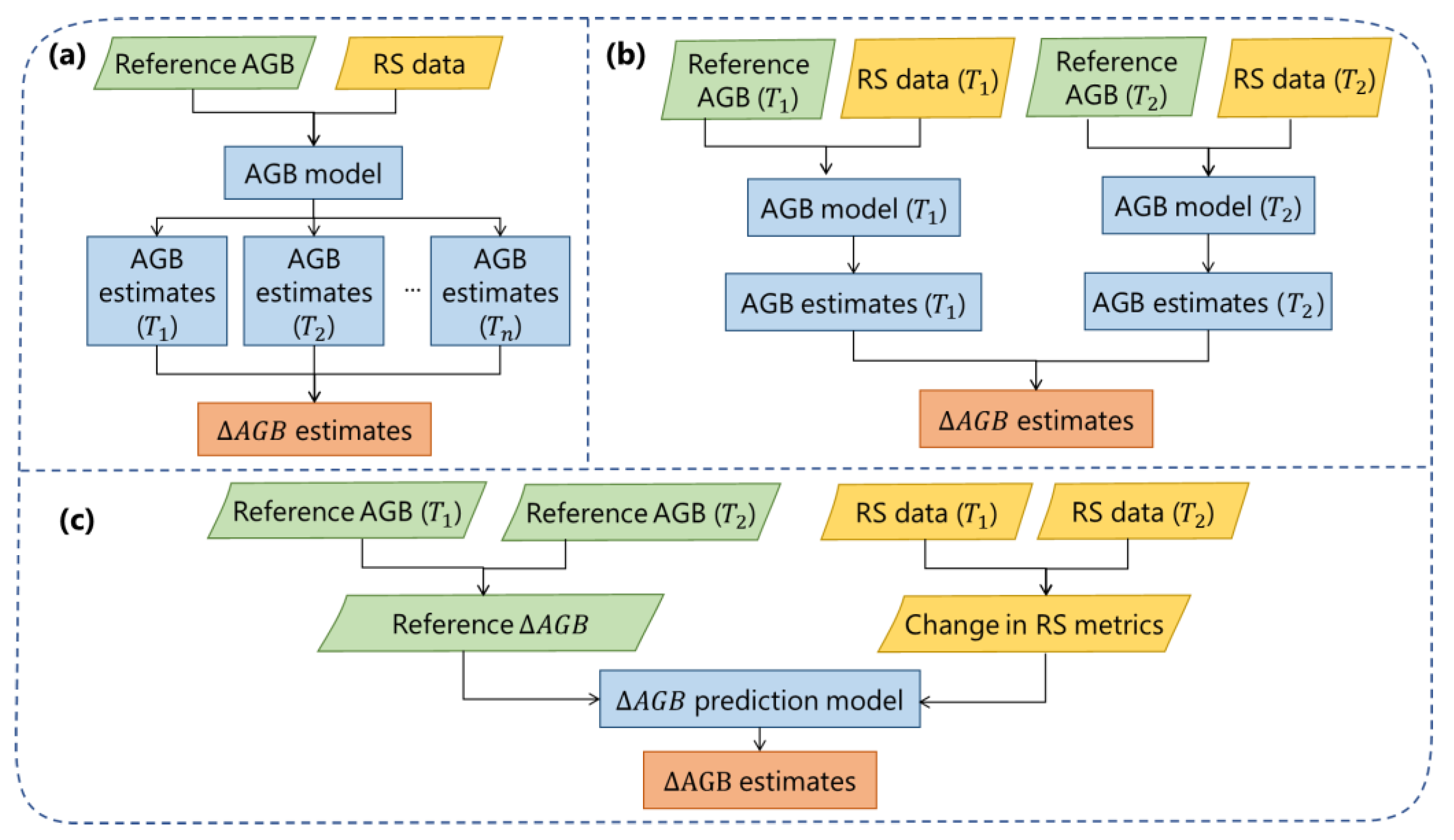
3. Direct and Indirect Methods for Estimating Biomass Changes

Methods for estimating forest AGB changes using multi-temporal remote sensing data can be broadly categorized into two approaches: direct estimation and indirect estimation (Figure 1). Among the selected literature, 116 articles employed indirect methods to estimate biomass change, 25 used direct methods, and 13 compared both approaches.

3.1. Direct Estimation Methods

Direct estimation involves establishing a direct relationship between AGB changes (∆AGB) and variations in remote sensing indices or metrics. This approach typically uses multi-temporal remote sensing data, such as ALS or satellite imagery, to quantify changes in forest structure and biomass.

For example, McRoberts et al. [65] applied several linear models to estimate ∆AGB based on changes in multi-temporal ALS metrics. Solberg et al. [51] applied a linear model to estimate ∆AGB directly from interferometric SAR height changes between SRTM and TanDEM-X. Johnson et al. [66] employed an integrated machine learning model to relate plot-level AGB to multi-temporal spectral indices as well as perturbation indicators from Landsat, producing historical AGB with fine spatiotemporal resolution.

Direct estimation methods require repeated observations to generate numerous ∆AGB samples for model training, which limits their applicability in regions with sparse observations. These methods are highly effective in capturing complex relationships in AGB changes but are heavily dependent on data availability.

3.2. Indirect Estimation Methods

When repeated observations are scarce, indirect estimation methods provide an alternative approach for assessing AGB changes [67]. If reference AGB values and corresponding remote sensing data are available for a given period, researchers can develop prediction models to estimate biomass across multiple periods and then quantify biomass changes using methods such as differential analysis, trend analysis, or curve fitting. For instance, Liu et al. [55] established a relationship between Saatchi AGB and average VOD to estimate forest AGB from 1993 to 2012, analyzing trends and inter-annual variations. Similarly, Baccini et al. [14] developed an RF model based on single-period biomass data to produce annual AGC estimates from 2003 to 2014, and then conducted change-point analysis to identify temporal trends. In some cases, biomass reference data from multiple years were aggregated to improve model training. Burrell et al. [68] combined field measurements from 25,000 forest plots with geospatial data and used machine learning models with site and interval withholding ensemble techniques to enhance predictive accuracy, achieving 70% accuracy in biomass loss estimation.

3.3. Applications and Comparison of Methods

Both direct and indirect methods for estimating biomass change have been applied across various forest types, including northern [39,45], temperate [69], subtropical [70], and tropical forests [5,24]. Some studies report higher accuracy with direct methods [70], while others favor indirect methods [65]. The specific conditions under which each method performs best remain uncertain. To investigate this, Knapp et al. [71] used the FORMIND model to simulate over 28,000 hectares of natural and disturbed forest stands, comparing direct and indirect methods. Their results indicated prediction accuracies of 18.7 t ha⁻¹ for direct estimation, 12.6 t ha⁻¹ for indirect estimation, and 12.4 t ha⁻¹ for an enhanced direct estimation method incorporating canopy texture.

4. Driving Factors of Biomass and Carbon Losses

Biomass change is driven by a complex interplay of both environmental and anthropogenic factors. Natural drivers such as climate change and disturbances (e.g., wildfires) significantly affect biomass [72,73], and human activities—particularly deforestation, land-use change, and logging—are leading contributors to biomass loss, particularly in tropical regions [74,75]. A comprehensive understanding of these drivers and their interactions is crucial for effective forest management, conservation strategies, and climate change mitigation efforts.

4.1. Climate Change

Climate change influences biomass through rising temperatures, altered precipitation patterns and an increase in extreme weather events. The impact of elevated atmospheric CO₂ concentrations and warming temperatures on forest biomass is complex and multifaceted. Increased CO₂ generally enhances photosynthesis, boosting plant productivity by improving carbon assimilation and water-use efficiency [76,77]. However, the long-term benefits of CO₂ fertilization are often constrained by nutrient limitations, species-specific physiological responses, and ecosystem feedback, leading to uncertainty regarding the overall impact [78].

Warmer temperatures also influence biomass by altering phenology, extending growing seasons, and shifting species distributions [79]. While warmer conditions can enhance productivity in temperate and boreal regions [80], they can also exacerbate heat stress and increase evapotranspiration, making forests more vulnerable to drought. For example, in Romania between 1987 and 2018, the direct effects of warming on AGB dynamics were minimal [81].

A shift in precipitation patterns is another crucial factor influencing biomass accumulation and carbon sequestration. Positive soil moisture and precipitation anomalies are generally associated with enhanced biomass accumulation, while negative anomalies lead to carbon losses [57]. In arid and semi-arid ecosystems, increased precipitation has been linked to biomass accumulation [82], whereas reduced precipitation can cause drought stress, decrease plant productivity and increase tree mortality [83].

Recent studies of Canada’s boreal forests using the TRIPLEX-Mortality model (1970–2020) highlight the significant role of drought in biomass loss. Following a sharp increase in drought-induced tree mortality around 2002, biomass declined at a rate of approximately 3.01 ± 0.58 Mg ha⁻¹ year⁻¹, with cumulative losses of approximately 0.93 ± 0.18 Pg C, primarily from aboveground biomass [84].

4.2. Natural Disturbances

Natural disturbances, including windthrows, wildfires, and insect outbreaks, play a significant role in shaping forest biomass dynamics. Windthrows, particularly those caused by storms, result in selective tree mortality and long-term biomass reductions. Even small–small windthrows, affecting 4%–20% of trees, can lead to biomass declines that last for decades, with recovery often requiring over 40 years [85].

A comprehensive assessment of European forests from 1979 to 2018 revealed that natural disturbances threaten approximately 33.4 billion tonnes of forest biomass, with windthrows accounting for 40% of biomass losses, followed by fires (34%) and insect outbreaks (26%) [86]. In the Amazon, natural disturbances contributed an estimated 1.30 Pg C annually, with small-scale mortality (<0.1 ha) contributing to ~98.6% of total carbon losses [87].

4.3. Human Drivers of Biomass Change

Human activities, particularly land-use changes and deforestation, play a significant role in shaping forest biomass and carbon stocks. Land-use and land-cover transformations can either enhance or reduce carbon storage, depending on the type of change [88]. Deforestation remains one of the primary drivers of biomass loss and carbon emissions, especially in tropical regions where large areas of forests are cleared for agriculture, significantly reducing biomass and carbon stocks [89]. The cumulative effects of deforestation and disturbance can convert forests into net carbon sources [14].

Forest degradation, often a consequence of deforestation, further exacerbates biomass loss. Fawcett et al. [90] observed that deforestation and associated degradation losses since 2012 has far outpaced recovery from secondary forest growth, with forest degradation accounting for 40% of total gross biomass losses. In the Brazilian Amazon, Qin et al. [91] reported a net AGB loss of 0.67 Pg C from 2010 to 2019, with forest degradation (73%) contributing three times more to biomass loss than deforestation (27%).

Deforestation also leads to forest fragmentation, which indirectly accelerates carbon loss from forest edges. Silva Junior et al. [92] quantified the additional carbon loss from forest edges in the Amazon, revealing that it accounted for one-third of carbon loss caused by deforestation between 2001 and 2015.

Selective logging is another significant driver of degradation, particularly in tropical forests. Pinagé et al. [93] assessed the impacts of logging in the Eastern Amazon using LiDAR data, finding substantial biomass reductions. However, other studies suggest that selectively logged forests can maintain biomass stability comparable to mature, conserved forests, provided logging does not lead to further degradation [94]. The long-term outcomes of selective logging depend on management practices. Sustainable forest management—including reduced-impact logging, controlled harvesting intensities, and extended rotation cycles—can mitigate biomass loss and even enhance carbon sequestration. For instance, Putz et al. [95] found that logged forests retaining 76% of original carbon stocks can recover to near pre-logging biomass levels within decades if collateral damage is minimized. Similarly, Edwards et al. [96] demonstrated that well-managed concessions retain 85%–100% of biodiversity and 70%–90% of biomass by protecting old-growth patches and riparian buffers. These practices, combined with silvicultural interventions, sustain timber yields and restore ecosystem functions.

4.4. Combined Effects of Natural and Anthropogenic Disturbances

Both natural and anthropogenic disturbances contribute significantly to carbon emissions from forest ecosystems. In Northern Ukraine, natural and human-induced disturbances accounted for nearly 21% of total carbon emissions from forest ecosystems between 2010 and 2015. Timber harvesting was responsible for 57% of emissions, followed by wind damage (34%), insect outbreaks (6%), and wildfires (3%) [97].

In Canada, a 33-year satellite-derived time series of AGB (1984–2016) revealed that undisturbed forests accrued 3.90 Pg of biomass, while disturbed forests lost 3.94 Pg. For the biomass reduction, 45.4% was attributed to wildfire, 43.8% to harvesting, 8.3% to non-stand replacing disturbances, and 2.5% to roads and infrastructure development [98]. In western North American boreal forests, fire, logging, and insect outbreaks resulted in average annual AGB losses of 23.4, 16.6, and 4.7 Tg, respectively [99].

4.5. Post-Disturbance Recovery and Biomass Regrowth

Forest ecosystems can recover following disturbances, potentially offsetting some of the carbon losses over decadal timescales. Requena Suarez et al. [100] found that Amazonian forests regained AGB at a rate of 4.7 Mg ha⁻¹ year⁻¹ during the first 20 years following disturbance. However, recovery rates vary significantly depending on the type of disturbance and local environmental conditions.

De Marzo et al. [101] showed that, 30 years post-disturbance, forests affected by natural disturbances (e.g., droughts, riparian changes) often exhibited higher AGB values than those impacted by anthropogenic disturbances, such as partial clearing and logging. Environmental factors such as vapor pressure deficit, soil clay content, temperature, and precipitation have been identified as key determinants of recovery following stand-replacing insect outbreaks and logging [99].

Additionally, forest canopy structure and prior AGB losses strongly influence recovery patterns [102]. However, disturbances can continue to act as carbon sources rather than sinks in some cases. Mackintosh et al. [103] found that lianas can hinder tree biomass recovery, contributing to further biomass declines, particularly through stem damage and delayed tree mortality.

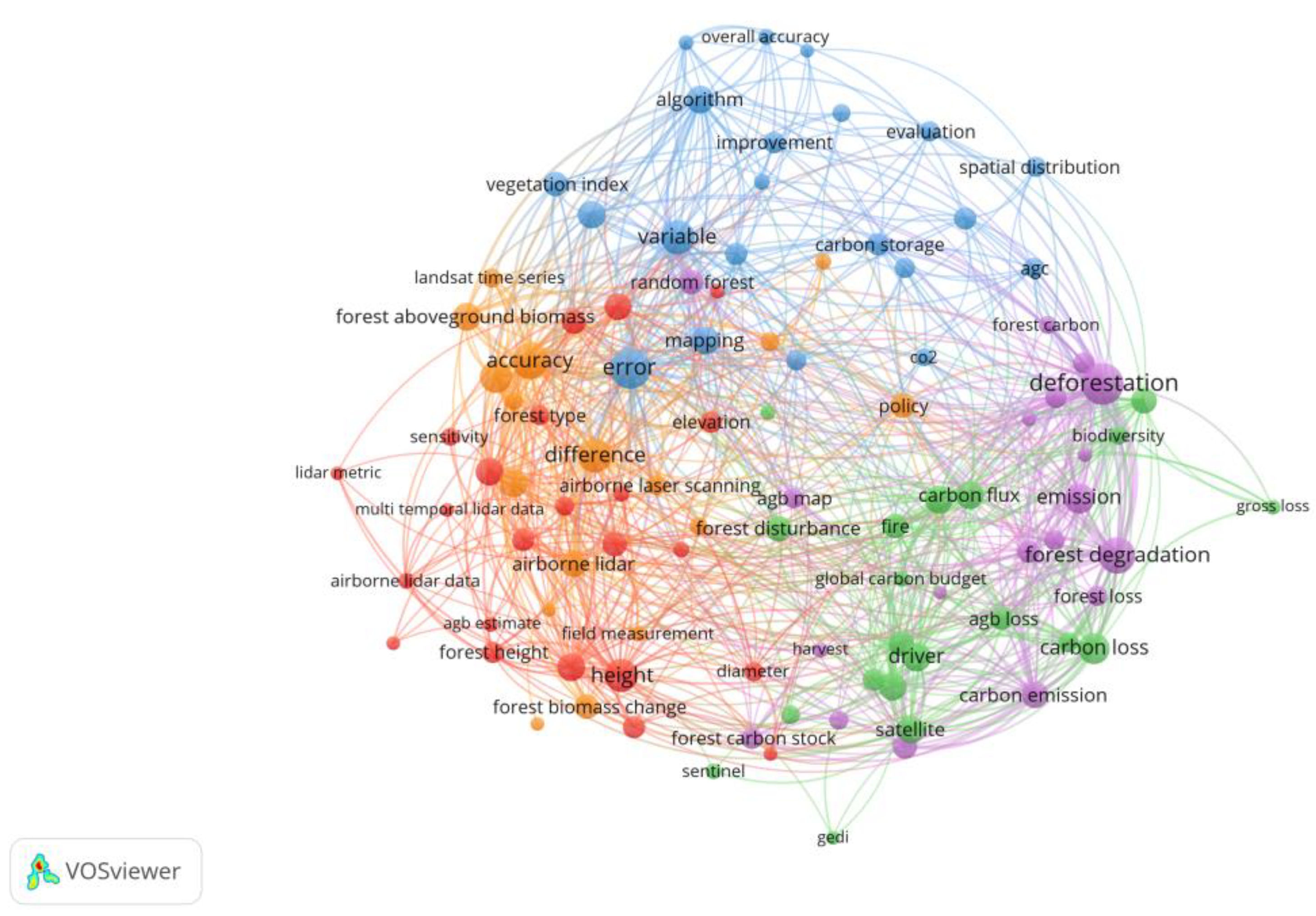
5. Meta-Analysis of Remote Sensing Studies on Forest Biomass Changes

5.1. Literature Sources

Figure 2 presents the number of annual publications from 2010 to 2024 for the selected 166 articles, highlighting an increase in studies over the past two years. Most publications (62.7%) were sourced from 13 peer-reviewed journals, as shown in Figure 3, with the remaining articles coming from a variety of journals. The two journals with the highest publication counts were Remote Sensing of Environment (16.3%) and Remote Sensing (15.7%), followed by Environmental Research Letters (4.2%) and Global Change Biology (4.2%).

5.2. Cluster Analysis

Cluster analysis was performed using VOSviewer version 1.6.20 [104] based on the frequency of terms extracted from the titles and abstracts of the selected articles. The binary counting method was applied, with a minimum occurrence threshold of five for each term. This analysis revealed five distinct research clusters, each corresponding to a key area of focus in forest biomass studies (Figure 4). These clusters were: the red cluster (23 terms), labeled “LiDAR and height”, which focused on the use of LiDAR technology for measuring forest height and biomass; the blue cluster (21 terms), labeled “Accuracy (concerned with accuracy in forest biomass mapping, including algorithms, variables, and methods for biomass estimation)”; the green cluster (20 terms), labeled “Biomass and carbon loss”; the purple cluster (19 terms), labeled “Disturbance (focusing on deforestation and forest degradation and their role in biomass loss)”; and the orange cluster (17 terms), labeled “Forest biomass and biomass change: accuracy, difference, and prediction”. The most frequently cited term in each cluster was “height” (22 occurrences), “error” (31 occurrences), “carbon loss” (20 occurrences), “deforestation” (33 occurrences), and “accuracy” (26 occurrences), respectively.

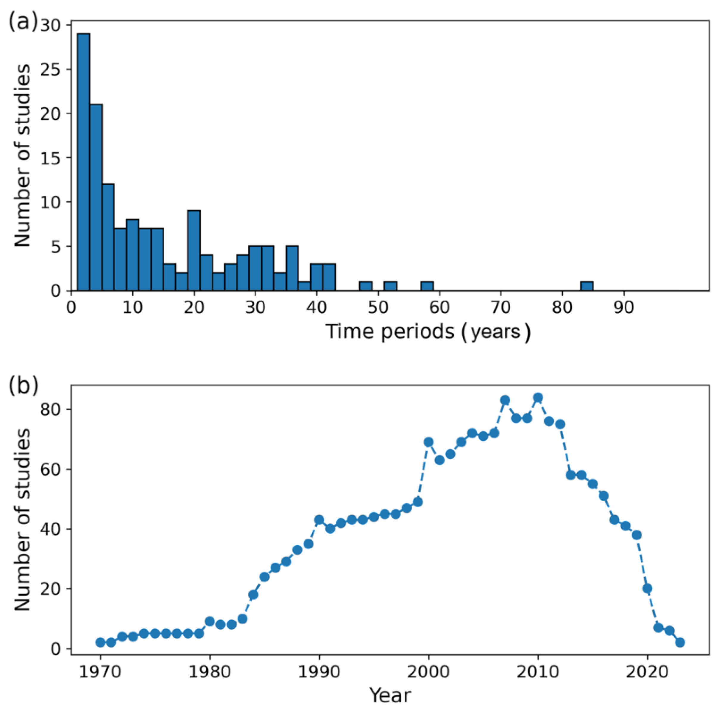
5.3. Spatial and Temporal Coverage

Biomass change studies exhibited significant geographical variation, as shown in Figure 5. In terms of geographical regions, Asia and North America had the highest concentration of biomass change studies, accounting for 29.7% and 22.2%, respectively, followed by Europe and South America. This distribution is closely linked to the importance of these forest ecosystems in global carbon sequestration [105].

At the country level, the United States and China were the most frequently studied nations. The Amazon region, being the world’s largest tropical rainforest, stands out as a major research hotspot due to its crucial role as a carbon sink and its rich biodiversity. Consequently, Brazil, Peru, and Colombia have emerged as the leading countries for biomass change studies.

In terms of temporal coverage, the majority of studies on forest biomass change spanned a period of 1 to 50 years, with over 140 studies conducted within this range (Figure 6). Most studies focused on biomass change across two periods or a few (e.g., three or four), rather than investigating long-term changes. This suggests that much of the published research emphasizes methodology development, which may not be sufficient for generating long-term biomass change maps at various scales. After filtering out years with only one study, the temporal distribution of studies reveals that research has been concentrated between 1980 and 2020, with a notable peak around 2010.

5.4. Spatial Resolution of Remote Sensing Data

As illustrated in Figure 7, 81.5% of studies focused on detecting biomass changes at spatial resolutions lower than 100 m, aligning with the use of Landsat and LiDAR data to capture fine-scale disturbances and AGB changes. In some cases, ALS and TLS were employed to assess biomass changes at the plot or tree level, corresponding to the high-resolution studies shown in Figure 7. In contrast, VOD-based biomass estimates or moderate-resolution optical imagery typically led to biomass estimates at resolutions larger than 100 m, with VOD-based methods accounting for most of these coarse-resolution studies.

5.5. Reference AGB Data

Among the 166 screened studies, 105 studies (63.3%) utilized field survey data as a reference for monitoring AGB changes with remote sensing techniques. For instance, some studies integrated field measurements with LiDAR data to explore its potential for monitoring forest dynamics (Section 2.1), while others combined field data with Landsat time series to quantify biomass changes (Section 2.2). Typically, the quantification of biomass and its changes involved using field survey data or ALS calibrated with field measurements as references. This approach is particularly suitable for small-scale, high-precision biomass estimation. Once calibrated, LiDAR data can be applied for large-scale biomass change monitoring, often in combination with optical imagery and SAR data, especially when field survey data are scarce [35,106]. For large-scale biomass change monitoring, coarse-resolution biomass maps are often used to develop relationships between VOD and AGB, enabling the generation of AGB maps over extensive areas [102,107].

5.6. Estimation Algorithms

A statistical analysis was conducted to evaluate the algorithms used for direct and indirect estimation methods. Among the most commonly used techniques, parametric regressions are widely used for estimating biomass change (Figure 8). To facilitate method selection and comparison, we have compiled and organized the parametric regression equations currently used in biomass change research (

Table 1. The structure of common parameter regression equations.

Model Type	Equation Forms	Reference
Linear	$y={\beta }_1{x}_1+{\beta }_2{x}_2+\cdots +{\beta }_n{x}_n+\epsilon$	[17]
	$∆y={\beta }_1(∆x_1)+{\beta }_2(∆x_2)+\cdots +{\beta }_n(∆x_n)+\epsilon$	[20]
Polynomial	$y={\beta }_1{x}_1+{\beta }_1{x}_2^{a_2}+\cdots +{\beta }_1{x}_n^{a_n}+\epsilon$	[49]
	$∆y={\beta }_1(∆x_1^{a_1})+{\beta }_2(∆x_2^{a_2})+\cdots +{\beta }_n(∆x_n^{a_n})+\epsilon$	[52]
Log-Transformed	$y={\beta }_1\ln \left(x\right)+\epsilon$	[49]
Logistic	$y={\displaystyle \frac{L}{1+e^{-\beta (x-x_0)}}}+\epsilon$	[108]
Multiplicative	$y={\beta }_0{∆x}_1^{{\beta }_1}{∆x}_2^{{\beta }_2}\cdots {∆x}_n^{{\beta }_n}$	[19]
Geographically Weighted Regression	$y={\beta }_0\left({\mu }_0, v_0\right)+{\displaystyle \sum _{k=1}^n}{\beta }_i\left({\mu }_i, v_i\right)x_{ik}+\epsilon$	[109]

). In these models, $y$ represents AGB at a given time; $∆y$ represents the change in AGB; $x_1$, $x_2$ and $x_n$ are the characteristic variables; $∆x_1$, $∆x_2$ and $∆x_3$ represent the changes in these variables and ${\beta }_1$, ${\beta }_2$ and ${\beta }_n$ are their respective coefficients; $\epsilon$ is the constant term. In the geographically weighted regression model, ${\beta }_0\left({\mu }_0, v_0\right)$ is the local intercept at the i-th position, which varies with its spatial position $\left({\mu }_0, v_0\right)$. ${\beta }_i\left({\mu }_i, v_i\right)$ represents the local regression coefficient of the i-th variable, reflecting its influence on AGB at spatial position $\left({\mu }_i, v_i\right)$. n denotes the number of predictor variables.

Specifically, linear regression models are frequently employed due to several reasons: (1) Linear relationships often exist between remote sensing-derived variables and AGB changes [110,111]; (2) The limited availability of field plots for measuring AGB change necessitates simpler modeling approaches [112]; and (3) Linear models offer better temporal transferability compared to complex machine learning models [113]. Although linear regression is widely used, it can sometimes lead to overly large positive or negative estimates. To mitigate this, some studies employed logistic models or alternative transformations [65].

Machine learning techniques, particularly for indirect estimation, can improve the accuracy of estimated biomass changes [67,114]. Among the machine learning algorithms, RF is the most widely used. Additionally, Support Vector Machines (SVM) [67], Multilayer Perceptron (MLP) [82] and XGBoost [69] are also employed for both direct and indirect biomass change estimation. However, the relationship between forest biomass and remote sensing data varies spatially and temporally, making it challenging for shallow machine learning methods to capture complex, nonlinear patterns. Deep learning algorithms offer superior pattern recognition and parameter estimation capabilities [115]. Various deep learning models, such as deep neural networks, stacked sparse autoencoders, and convolutional neural networks (CNN), have been applied for AGB estimation. However, the full application of deep learning models in biomass change estimation is still an area of ongoing research [116,117].

Some studies have also utilized allometric models to calculate biomass and its changes [118], while others have used parameters such as LiDAR-derived canopy cover to estimate biomass [119]. Additionally, ecological process models are sometimes applied to simulate biomass changes [120].

5.7. Comparison Studies

Of the 166 studies reviewed, 32 studies (19.3%) involved comparative analysis. Among these, 15 studies compared the effects of different data sources for estimating biomass changes. Since single data sources (e.g., optical imagery or radar data) suffer from issues such as signal saturation or topography effects, which limit the accuracy of AGB or AGB change estimates, many studies have suggested that multi-source data fusion can significantly improve the accuracy of biomass estimates. For example, Naesset [20] found that compared with relying solely on ground survey data, the inclusion of remote sensing data significantly improved the relative efficiency of the model. Pereira [121] found that the highest-performing biomass models integrated ALS, ALOS PALSAR (L-band HV polarization), Sentinel-1 (C-band) and Landsat-8 data. Additionally, Liu et al. [122] suggested that combining meteorological variables (precipitation and temperature) with Landsat spectral data led to a significant reduction in RMSE compared to using spectral variables alone.

However, introducing too many variables can lead to noise [43], which may reduce model accuracy. In such cases, model efficiency can be enhanced by screening feature variables using techniques like random forest or stepwise regression [123].

Regarding the comparison between direct and indirect methods for biomass change, most studies indicate that indirect methods generally provide higher accuracy [65,72,124], though some studies suggest that direct methods can offer better accuracy in certain contexts [70]. To address this discrepancy, recent studies have developed hybrid strategies. For example, Johnson et al. [66] used the weighted average of direct and indirect methods to predict results, while Knapp et al. [71] optimized the direct method using multivariate information and a RF algorithm.

In terms of model comparison, machine learning methods have demonstrated advantages in complex environments. RF [125,126] and XGBoost [119] tend to outperform traditional allometric equations in complex terrain and vegetation structures. However, Zhao et al. [23] pointed out that random forests may suffer from overfitting, leading to reduced accuracy in actual predictions. In contrast, parametric regression models [127,128] remain valuable, particularly in cases with small sample sizes or linear relationships. These findings suggest that selecting the optimal model requires a comprehensive assessment of data complexity, sample size, and research objectives.

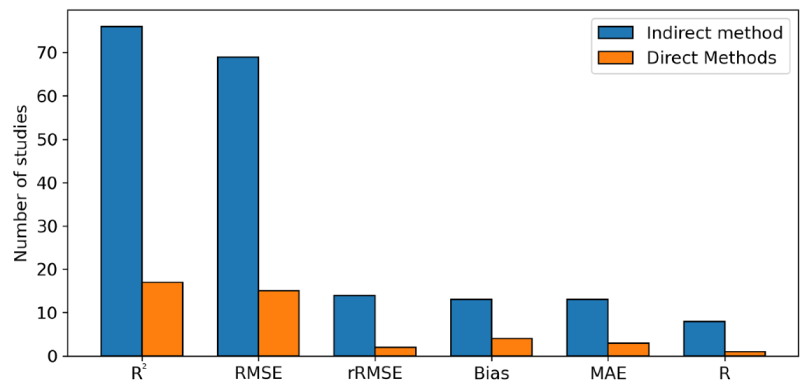
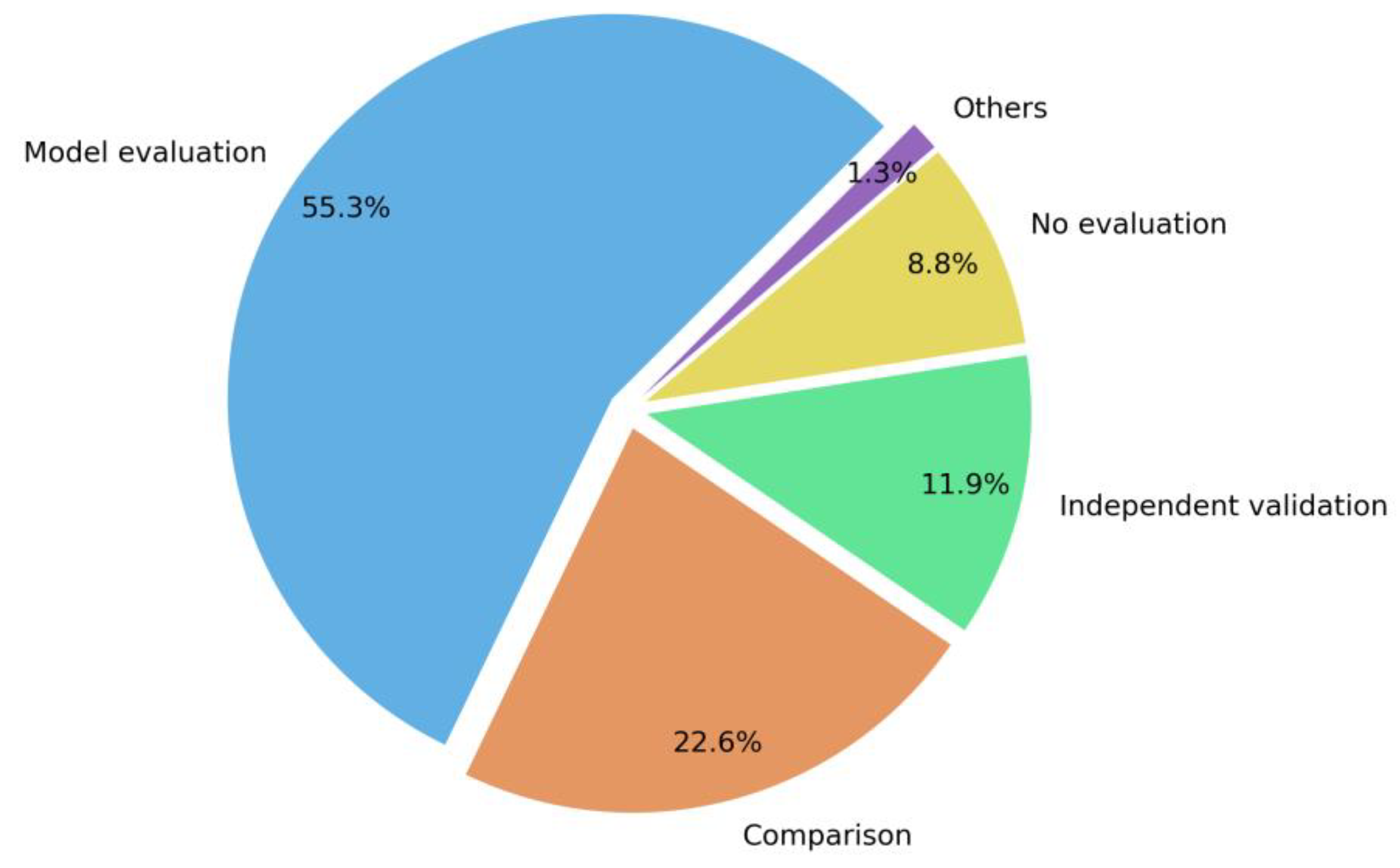
5.8. Accuracy Assessment

Various metrics were employed to assess the accuracy of biomass change estimates (Figure 9). The most frequently used metrics included:

R² (Coefficient of Determination):

$$R^2=1-{\displaystyle \frac{{\sum }_{i=1}^n{(y_i-{\widehat{y}}_i)}^2}{{\sum }_{i=1}^n{(y_i-{\overline{y}}_i)}^2}}$$

(1)

RMSE (Root Mean Square Error):

$$RMSE=\sqrt{{\displaystyle \frac{1}{n}}\sum _{i=1}^n{(y_i-{\widehat{y}}_i)}^2}$$

(2)

rRMSE (Relative RMSE):

$$rRMSE={\displaystyle \frac{RMSE}{\overline{y}}}\times 100\%$$

(3)

Bias:

$$Bias={\displaystyle \frac{1}{n}}\sum _{i=1}^n({\widehat{y}}_i-y_i)$$

(4)

MAE (Mean Absolute Error):

$$MAE={\displaystyle \frac{1}{n}}\sum _{i=1}^n|{\widehat{y}}_i-y_i|$$

(5)

R (Pearson Correlation Coefficient):

$$R={\displaystyle \frac{\sum _{i=1}^n(y_i-{\overline{y}}_i)\sum _{i=1}^n(y_i-{\widehat{y}}_i)}{\sqrt{\sum _{i=1}^n{(y_i-{\overline{y}}_i)}^2}\sqrt{\sum _{i=1}^n{(y_i-{\widehat{y}}_i)}^2}}}$$

(6)

where $y_i$ is the observed value, ${\widehat{y}}_i$ is the predicted value, and ${\overline{y}}_i$ is the mean value of observations.

Many studies, especially those using indirect methods, focused on estimating biomass at specific points in time, with the prediction accuracy typically referring to biomass estimates at those times rather than the changes in biomass over time.

As shown in Figure 10, only 11.9% of the studies employed independent validation to evaluate the prediction accuracy. About 22.6% of studies relied on comparisons or inter-comparisons with other results to assess the reasonableness of the estimates. Others indicated that indirect evaluations, such as assessing relevance with REDD+ [129], were used. Finally, 8.8% of studies did not perform any evaluation of their results.

Most studies (55.3%) used a train–test split strategy, sometimes combined with cross-validation, where the data are partitioned into training and test sets. The test set is used to assess the overall model prediction accuracy, which primarily evaluates the model’s generalization ability, distinct from the validation of biomass change estimates.

A significant limitation is the scarcity of reference biomass change data, such as from permanent plots, making it difficult to accurately assess biomass change estimates. Most studies used limited sample sizes for accuracy assessment, often constrained to small, localized areas. This further complicates large-scale, regional assessments and contributes to the uncertainties in biomass change estimates.

6. Discussion

6.1. Factors Influencing the Accuracy of Biomass Change Estimation

Both indirect and direct estimation methods offer valuable insights into biomass changes, but each comes with limitations that affect their accuracy and reliability. Indirect methods, which often rely on time-series optical remote sensing or LiDAR data, face challenges related to sensor variability, atmospheric effects, seasonal fluctuations, and other sources of noise that can degrade biomass estimates [130,131]. Direct approaches are heavily dependent on the availability and quality of reference data on AGB changes, such as data from ground plots or other reliable sources. The accuracy of direct methods is also influenced by the representativeness of field measurements [132,133].

A critical factor that influences accuracy in both methods is the sample size and plot size used for estimation. Several studies have shown that increasing the plot size (from 314 m² to 1964 m²) significantly improves the biomass prediction accuracy, with R² improving from 0.92 to 0.97. Larger plots (1000 m² or 1964 m²) have a higher degree of spatial overlap with ground-reference data, making them less prone to co-registration errors compared to smaller plots [134]. Moreover, larger plots tend to exhibit lower estimation errors that are less sensitive to plot location errors and varying vegetation conditions [134,135]. Tao et al. [136] quantified the accuracy of AGB estimates from Landsat imagery at progressively larger spatial scales. Their results revealed a monotonic relationship, where accuracy improved with increasing spatial scale up to 60–90 m, after which it declined. Based on these findings, they recommended using a spatial scale of 60–90 m for forest AGB estimation using Landsat data.

The choice of prediction method also has a profound effect on accuracy. Several studies suggested that the selection of the prediction method may influence the results more than sample size [136], highlighting the importance of carefully selecting the appropriate modeling approach based on the spatial and temporal characteristics of the remote sensing data. Only 6.6% of studies in this review compared different algorithms to select the optimal prediction method. Future research should consider deep learning approaches, which can effectively capture non-linear relationships in multi-temporal data, enhancing the robustness against noise and missing observations [115]. Ge et al. [137] showed that Long Short-Term Memory (LSTM) networks combined with fully connected neural networks improved biomass predictions (R² = 0.63) by using time-series Landsat data to capture disturbance and recovery dynamics. Data fusion techniques, such as combining Gaofen SAR, Sentinel, and ALOS-2 data with CNN-LSTM frameworks, have also enhanced biomass estimate accuracy by leveraging both temporal and spectral information [138]. Additionally, hybrid models integrating process-based ecological models with machine learning could improve long-term AGB projections by accounting for environmental drivers and should be explored in future studies [139].

6.2. Challenges and Limitations of Monitoring Forest AGB with Remote Sensing

Despite significant advancements in using remote sensing data to estimate forest biomass and its dynamics, several challenges remain that hinder the accuracy and applicability of biomass change monitoring. In the case of multispectral remote sensing, the role of incorporating longer time series, as well as seasonal or phenological data, to improve the accuracy of biomass change assessments remains underexplored. While leaf phenology plays a well-established role in influencing ecosystem properties, studies by Wang et al. [140] suggest that AGB is more strongly influenced by functional trait composition and taxonomic diversity than by leaf phenological diversity [141]. This highlights the need for further research into the interaction between phenological patterns and biomass dynamics.

Cloud cover is a persistent problem in tropical regions, where acquiring cloud-free imagery for biomass change detection is often a significant challenge. The low spatial and temporal resolution of some remote sensing data can also impede the accurate tracking of biomass changes, particularly for large-scale studies [142,143]. The use of very high-resolution imagery comes with issues of cost and scalability that limit its applicability for large-scale biomass monitoring [144,145].

While multi-temporal LiDAR surveys are increasingly employed to analyze forest AGB changes, their full potential for assessing disturbances—critical for understanding forest dynamics and biomass loss—has not been fully realized [146]. New LiDAR missions such as GEDI, ICESat-2, and upcoming missions provide exciting new opportunities for high-resolution, global biomass change monitoring. These advancements are particularly beneficial for carbon cycle assessments, REDD+ initiatives, and forest conservation strategies. Another promising yet challenging approach involves the use of VOD for biomass estimation. While VOD-based methods have proven effective for global forest dynamics monitoring, several challenges remain. The most significant of these is the relatively coarse spatial resolution of VOD data (e.g., 0.25°), which limits its effectiveness for fine-scale biomass monitoring. The non-linear relationship between VOD and AGB makes it difficult to apply simple regression models for biomass estimation. Although advanced statistical methods and machine learning approaches could improve biomass estimates, these techniques have been underexplored in the context of VOD-based estimations. Despite these limitations, the integration of VOD data with other remote sensing technologies offers substantial promise for enhancing global biomass monitoring. As satellite missions continue to improve VOD resolution and accuracy, the potential to track biomass changes on global, regional, and local scales will expand, providing new opportunities for frequent and more accurate biomass change detection.

While remote sensing can effectively measure AGB at large scales, estimating below-ground biomass (BGB) presents greater challenges. A single model often struggles to capture the heterogeneity of BGB across different vegetation types, leading to systematic over- or underestimation [147]. Although some studies have used LiDAR and microwave remote sensing technologies for BGB estimation, their performance remains limited. For instance, GEDI data achieves an R² of 0.37–0.59 for BGB monitoring [148]. Overall, current BGB estimation methods perform well in small-scale or homogeneous forests, but face significant challenges in large, diverse, or complex environments due to issues like low accuracy, high cost, and limited technical adaptability.

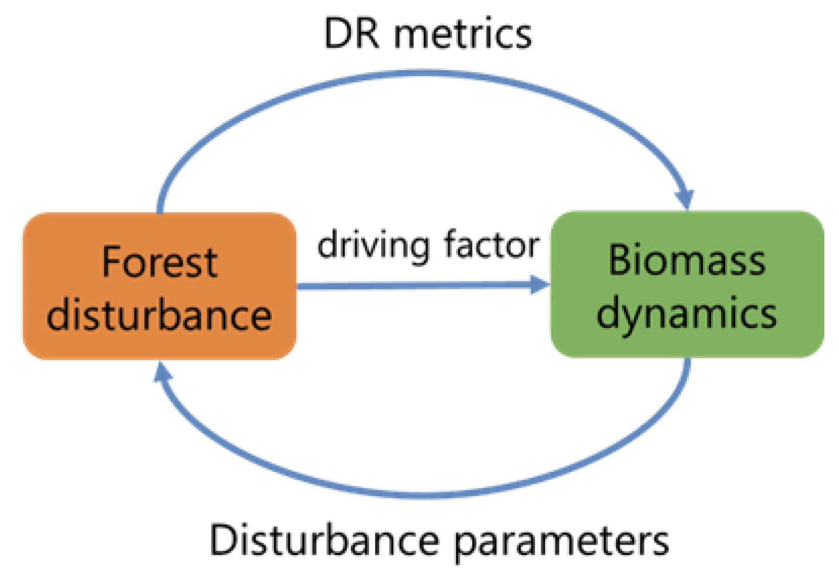
6.3. Forest Disturbance and Forest Biomass Dynamics

As highlighted in Section 4, forest disturbances have a significant impact on biomass dynamics. The relationship between disturbance and biomass change is multifaceted (Figure 11). DR metrics can be integrated into biomass monitoring to enhance accuracy. These metrics help capture both the extent of disturbances and subsequent recovery of biomass over time, which can refine estimates of forest carbon stocks [44]. Similarly, disturbance can also be directly identified and quantified from remotely sensed biomass maps. These maps provide critical data to estimate disturbance parameters, such as the probability of disturbance occurring in a specific forest patch and the intensity of the disturbance [6]. Remote sensing technologies thus not only provide valuable insights into the temporal and spatial patterns of biomass change but also improve the ability to model disturbance effects on forest ecosystems at large scales.

6.4. Combination of Remote Sensing with Other Disciplines

Despite significant progress having been made in monitoring forest biomass using remote sensing, these data typically cover shorter timeframes compared to the long-term processes of forest succession and environmental changes [149,150]. This temporal limitation means that remote sensing data alone may not fully capture the dynamics of forest AGB and the underlying ecological processes that govern them.

To overcome this limitation, ecological models are often used to simulate long-term biomass dynamics. However, the accuracy of these models can be hindered by the complexity of ecological processes, uncertainties in input data, and potential flaws in model assumptions [151,152]. As a result, several studies have combined remote sensing with process-based models to enhance our understanding of forest biomass dynamics. For instance, Lu et al. [153] successfully integrated remote sensing-based AGB estimates as the initial carbon pool to parameterize the Boreal Ecosystem Productivity Simulator (BEPS) model, effectively updating the spatiotemporal distribution of forest AGB. Another example of this integrated approach is the National Forest Carbon Monitoring System (NFCMS), which combines forest inventory data, satellite remote sensing of stand biomass and forest disturbances, and an ecosystem carbon cycle model. This system has enabled the spatially explicit estimation of carbon stocks and fluxes from 1986 to 2010 [154]. Such approaches have proven effective in providing accurate assessments of biomass dynamics at regional scales.

Additionally, integrated approaches are commonly used to estimate forest carbon loss and gain. For example, models that combine biomass maps with land cover change have been used to quantify AGB variations [155,156]. Similarly, Hiltner et al. [157] integrated forest models with remote sensing data to quantify biomass loss and reduce uncertainties in global carbon cycle analysis.

7. Conclusions

Remote sensing technology holds significant promise for monitoring AGB in forests. This paper outlined recent advancements in remote sensing technologies, AGB estimation models, and the driving factors of biomass changes, while also addressing the challenges and potential future directions to resolve these issues. The key conclusions are summarized as follows.

A long temporal span (e.g., 10–30 years) is essential for monitoring AGB changes. Time series data enable detection of biomass change trends, identification of factors influencing biomass dynamics, and monitoring of forest recovery after disturbance. Longer time-series also improve AGB estimation accuracy through predictors like disturbance indices. To fully leverage these datasets, advanced modeling approaches are needed, moving beyond conventional methods like parametric models or random forests. Future research should explore cutting-edge algorithms, such as nonlinear parametric regressions (e.g., asymptotic or logistic growth models) and mixed-effects models to handle hierarchical data and temporal dependencies. Additionally, modern AI techniques like transformers for temporal pattern recognition, Bayesian neural networks for uncertainty quantification, and physics-informed machine learning can further enhance both accuracy and ecological interpretability.

A comprehensive validation framework is lacking in remote sensing-based AGB estimation. While these estimates are widely used, few studies incorporate independent validation using ground-based measurements, particularly from repeated or permanent sample plots to assess their accuracy. Such field-based validation is crucial not only for assessing the accuracy of spatiotemporal AGB models but also for advancing our understanding of long-term biomass dynamics, disturbance recovery, and carbon sequestration. As remote sensing becomes increasingly relied upon for large-scale AGB monitoring, prioritizing a robust validation framework that integrates remote sensing with continuous field measurements is essential to ensure both methodological reliability and ecological relevance.

A combination of remote sensing with other complementary techniques such as ecological models is needed to enhance estimation accuracy, extend the temporal coverage, and gain a deeper understanding of the factors driving AGB changes.

In conclusion, ongoing advancements in remote sensing technology, coupled with refined modeling approaches, improved validation methodologies, and integration with other analytical techniques, offer promising avenues for enhancing our understanding of AGB dynamics. These advancements are crucial for understanding the implications of AGB dynamics for forest ecosystems and carbon cycling.

References

1. Houghton, R.A. Aboveground Forest Biomass and the Global Carbon Balance. Glob. Change Biol. 2005, 11, 945–958. [Google Scholar] [CrossRef]
2. GCOS. The Global Observing System for Climate: Implementation Needs; World Meteorological Organization: Geneva, Switzerland, 2016; Volume GCOS-200, p. 341. [Google Scholar]
3. Bojinski, S.; Verstraete, M.; Peterson, T.C.; Richter, C.; Simmons, A.; Zemp, M. The Concept of Essential Climate Variables in Support of Climate Research, Applications, and Policy. Bull. Am. Meteorol. Soc. 2014, 95, 1431–1443. [Google Scholar] [CrossRef]
4. Vanderwel, M.C.; Coomes, D.A.; Purves, D.W. Quantifying variation in forest disturbance, and its effects on aboveground biomass dynamics, across the eastern United States. Glob. Change Biol. 2013, 19, 1504–1517. [Google Scholar] [CrossRef] [PubMed]
5. Zhang, Y.; Liang, S. Changes in forest biomass and linkage to climate and forest disturbances over Northeastern China. Glob. Change Biol. 2014, 20, 2596–2606. [Google Scholar] [CrossRef] [PubMed]
6. Williams, M.; Hill, T.C.; Ryan, C.M. Using biomass distributions to determine probability and intensity of tropical forest disturbance. Plant Ecol. Divers. 2013, 6, 87–99. [Google Scholar] [CrossRef]
7. Marvin, D.C.; Asner, G.P.; Knapp, D.E.; Anderson, C.B.; Martin, R.E.; Sinca, F.; Tupayachi, R. Amazonian landscapes and the bias in field studies of forest structure and biomass. Proc. Natl. Acad. Sci. USA 2014, 111, E5224–E5232. [Google Scholar] [CrossRef]
8. Lu, D.; Chen, Q.; Wang, G.; Liu, L.; Li, G.; Moran, E. A survey of remote sensing-based aboveground biomass estimation methods in forest ecosystems. Int. J. Digit. Earth 2016, 9, 63–105. [Google Scholar] [CrossRef]
9. Saatchi, S.S.; Harris, N.L.; Brown, S.; Lefsky, M.; Mitchard, E.T.A.; Salas, W.; Zutta, B.R.; Buermann, W.; Lewis, S.L.; Hagen, S.; et al. Benchmark map of forest carbon stocks in tropical regions across three continents. Proc. Natl. Acad. Sci. USA 2011, 108, 9899–9904. [Google Scholar] [CrossRef]
10. Liang, M.; Duncanson, L.; Silva, J.A.; Sedano, F. Quantifying aboveground biomass dynamics from charcoal degradation in Mozambique using GEDI Lidar and Landsat. Remote Sens. Environ. 2023, 284, 113367. [Google Scholar] [CrossRef]
11. Zhang, Y.; Liang, S.; Yang, L. A Review of Regional and Global Gridded Forest Biomass Datasets. Remote Sens. 2019, 11, 2744. [Google Scholar] [CrossRef]
12. Rodríguez-Veiga, P.; Wheeler, J.; Louis, V.; Tansey, K.; Balzter, H. Quantifying Forest Biomass Carbon Stocks From Space. Curr. For. Rep. 2017, 3, 1–18. [Google Scholar] [CrossRef]
13. Herold, M.; Carter, S.; Avitabile, V.; Espejo, A.B.; Jonckheere, I.; Lucas, R.; McRoberts, R.E.; Næsset, E.; Nightingale, J.; Petersen, R.; et al. The Role and Need for Space-Based Forest Biomass-Related Measurements in Environmental Management and Policy. Surv. Geophys. 2019, 40, 757–778. [Google Scholar] [CrossRef]
14. Baccini, A.; Walker, W.; Carvalho, L.; Farina, M.; Sulla-Menashe, D.; Houghton, R.A. Tropical forests are a net carbon source based on aboveground measurements of gain and loss. Science 2017, 358, 230–234. [Google Scholar] [CrossRef]
15. Araza, A.; Herold, M.; de Bruin, S.; Ciais, P.; Gibbs, D.A.; Harris, N.; Santoro, M.; Wigneron, J.P.; Yang, H.; Málaga, N.; et al. Past decade above-ground biomass change comparisons from four multi-temporal global maps. Int. J. Appl. Earth Obs. Geoinf. 2023, 118, 103274. [Google Scholar] [CrossRef]
16. Zhang, Y.; Ling, F.; Wang, X.; Foody, G.M.; Boyd, D.S.; Li, X.; Du, Y.; Atkinson, P.M. Tracking small-scale tropical forest disturbances: Fusing the Landsat and Sentinel-2 data record. Remote Sens. Environ. 2021, 261, 112470. [Google Scholar] [CrossRef]
17. Frolking, S.; Palace, M.W.; Clark, D.B.; Chambers, J.Q.; Shugart, H.H.; Hurtt, G.C. Forest disturbance and recovery: A general review in the context of spaceborne remote sensing of impacts on aboveground biomass and canopy structure. J. Geophys. Res. Biogeosci. 2009, 114, G00E02. [Google Scholar] [CrossRef]
18. Polanin, J.R.; Pigott, T.D.; Espelage, D.L.; Grotpeter, J.K. Best practice guidelines for abstract screening large-evidence systematic reviews and meta-analyses. Res. Synth. Methods 2019, 10, 330–342. [Google Scholar] [CrossRef]
19. Naesset, E.; Bollandsas, O.M.; Gobakken, T.; Gregoire, T.G.; Stahl, G. Model-assisted estimation of change in forest biomass over an 11 year period in a sample survey supported by airborne LiDAR: A case study with post-stratification to provide “activity data”. Remote Sens. Environ. 2013, 128, 299–314. [Google Scholar] [CrossRef]
20. Naesset, E.; Bollandsas, O.M.; Gobakken, T.; Solberg, S.; McRoberts, R.E. The effects of field plot size on model-assisted estimation of aboveground biomass change using multitemporal interferometric SAR and airborne laser scanning data. Remote Sens. Environ. 2015, 168, 252–264. [Google Scholar] [CrossRef]
21. Hudak, A.T.; Strand, E.K.; Vierling, L.A.; Byrne, J.C.; Eitel, J.U.H.; Martinuzzi, S.; Falkowski, M.J. Quantifying aboveground forest carbon pools and fluxes from repeat LiDAR surveys. Remote Sens. Environ. 2012, 123, 25–40. [Google Scholar] [CrossRef]
22. Simonson, W.; Ruiz-Benito, P.; Valladares, F.; Coomes, D. Modelling above-ground carbon dynamics using multi-temporal airborne lidar: Insights from a Mediterranean woodland. Biogeosciences 2016, 13, 961–973. [Google Scholar] [CrossRef]
23. Zhao, K.; Suarez, J.C.; Garcia, M.; Hu, T.; Wang, C.; Londo, A. Utility of multitemporal lidar for forest and carbon monitoring: Tree growth, biomass dynamics, and carbon flux. Remote Sens. Environ. 2018, 204, 883–897. [Google Scholar] [CrossRef]
24. Dubayah, R.O.; Sheldon, S.L.; Clark, D.B.; Hofton, M.A.; Blair, J.B.; Hurtt, G.C.; Chazdon, R.L. Estimation of tropical forest height and biomass dynamics using lidar remote sensing at La Selva, Costa Rica. J. Geophys. Res. Biogeosci. 2010, 115, G00E09. [Google Scholar] [CrossRef]
25. Meyer, V.; Saatchi, S.S.; Chave, J.; Dalling, J.; Bohlman, S.; Fricker, G.A.; Robinson, C.; Neumann, M. Detecting tropical forest biomass dynamics from repeated airborne Lidar measurements. Biogeosciences 2013, 10, 5421–5438. [Google Scholar] [CrossRef]
26. Rejou-Mechain, M.; Tymen, B.; Blanc, L.; Fauset, S.; Feldpausch, T.R.; Monteagudo, A.; Phillips, O.L.; Richard, H.; Chave, J. Using repeated small-footprint LiDAR acquisitions to infer spatial and temporal variations of a high-biomass Neotropical forest. Remote Sens. Environ. 2015, 169, 93–101. [Google Scholar] [CrossRef]
27. De Moura, Y.M.; Balzter, H.; Galvão, L.S.; Dalagnol, R.; Espírito-Santo, F.; Santos, E.G.; Garcia, M.; Bispo, P.C.; Oliveira, R.C.; Shimabukuro, Y.E. Carbon dynamics in a human-modified tropical forest: A case study using multi-temporal LiDAR data. Remote Sens. 2020, 12, 430. [Google Scholar] [CrossRef]
28. Srinivasan, S.; Popescu, S.C.; Eriksson, M.; Sheridan, R.D.; Ku, N.-W. Multi-temporal terrestrial laser scanning for modeling tree biomass change. For. Ecol. Manag. 2014, 318, 304–317. [Google Scholar] [CrossRef]
29. Turner, S.B.; Turner, D.P.; Gray, A.N.; Fellers, W. An approach to estimating forest biomass change over a coniferous forest landscape based on tree-level analysis from repeated lidar surveys. Int. J. Remote Sens. 2019, 40, 2558–2575. [Google Scholar] [CrossRef]
30. Krooks, A.; Kaasalainen, S.; Kankare, V.; Joensuu, M.; Raumonen, P.; Kaasalainen, M. Predicting tree structure from tree height using terrestrial laser scanning and quantitative structure models. Silva Fenn. 2014, 48, 1125. [Google Scholar] [CrossRef]
31. Simard, M.; Pinto, N.; Fisher, J.B.; Baccini, A. Mapping forest canopy height globally with spaceborne lidar. J. Geophys. Res. Biogeosci. 2011, 116, G04021. [Google Scholar] [CrossRef]
32. Hu, T.; Su, Y.; Xue, B.; Liu, J.; Zhao, X.; Fang, J.; Guo, Q. Mapping Global Forest Aboveground Biomass with Spaceborne LiDAR, Optical Imagery, and Forest Inventory Data. Remote Sens. 2016, 8, 565. [Google Scholar] [CrossRef]
33. Neuenschwander, A.; Pitts, K. The ATL08 land and vegetation product for the ICESat-2 Mission. Remote Sens. Environ. 2019, 221, 247–259. [Google Scholar] [CrossRef]
34. Dubayah, R.; Armston, J.; Healey, S.P.; Bruening, J.M.; Patterson, P.L.; Kellner, J.R.; Duncanson, L.; Saarela, S.; Ståhl, G.; Yang, Z.; et al. GEDI launches a new era of biomass inference from space. Environ. Res. Lett. 2022, 17, 095001. [Google Scholar] [CrossRef]
35. Xu, L.; Saatchi, S.S.; Yang, Y.; Yu, Y.; Pongratz, J.; Bloom, A.A.; Bowman, K.; Worden, J.; Liu, J.; Yin, Y.; et al. Changes in global terrestrial live biomass over the 21st century. Sci. Adv. 2021, 7, eabe9829. [Google Scholar] [CrossRef]
36. Wulder, M.A.; Coops, N.C. Satellites: Make Earth observations open access. Nature 2014, 513, 30–31. [Google Scholar] [CrossRef] [PubMed]
37. Wulder, M.; Loveland, T.; Roy, D.; Crawford, C.; Masek, J.; Woodcock, C.; Allen, R.; Anderson, M.; Belward, A.; Cohen, W.; et al. Current status of Landsat program, science, and applications. Remote Sens. Environ. 2019, 225, 127–147. [Google Scholar] [CrossRef]
38. Keeley, J. Fire intensity, fire severity and burn severity: A brief review and suggested usage. Int. J. Wildland Fire 2009, 18, 116–126. [Google Scholar] [CrossRef]
39. Gao, B.-C. NDWI—A normalized difference water index for remote sensing of vegetation liquid water from space. Remote Sens. Environ. 1996, 58, 257–266. [Google Scholar] [CrossRef]
40. Huang, C.; Goward, S.N.; Masek, J.G.; Thomas, N.; Zhu, Z.; Vogelmann, J.E. An automated approach for reconstructing recent forest disturbance history using dense Landsat time series stacks. Remote Sens. Environ. 2010, 114, 183–198. [Google Scholar] [CrossRef]
41. Ma, Q.; Su, Y.; Luo, L.; Li, L.; Kelly, M.; Guo, Q. Evaluating the uncertainty of Landsat-derived vegetation indices in quantifying forest fuel treatments using bi-temporal LiDAR data. Ecol. Indic. 2018, 95, 298–310. [Google Scholar] [CrossRef]
42. Powell, S.L.; Cohen, W.B.; Healey, S.P.; Kennedy, R.E.; Moisen, G.G.; Pierce, K.B.; Ohmann, J.L. Quantification of live aboveground forest biomass dynamics with Landsat time-series and field inventory data: A comparison of empirical modeling approaches. Remote Sens. Environ. 2010, 114, 1053–1068. [Google Scholar] [CrossRef]
43. Main-Knorn, M.; Cohen, W.B.; Kennedy, R.E.; Grodzki, W.; Pflugmacher, D.; Griffiths, P.; Hostert, P. Monitoring coniferous forest biomass change using a Landsat trajectory-based approach. Remote Sens. Environ. 2013, 139, 277–290. [Google Scholar] [CrossRef]
44. Pflugmacher, D.; Cohen, W.B.; Kennedy, R.E.; Yang, Z. Using Landsat-derived disturbance and recovery history and lidar to map forest biomass dynamics. Remote Sens. Environ. 2014, 151, 124–137. [Google Scholar] [CrossRef]
45. Puliti, S.; Breidenbach, J.; Schumacher, J.; Hauglin, M.; Klingenberg, T.F.; Astrup, R. Above-ground biomass change estimation using national forest inventory data with Sentinel-2 and Landsat. Remote Sens. Environ. 2021, 265, 112644. [Google Scholar] [CrossRef]
46. Soja, M.J.; Quegan, S.; d’Alessandro, M.M.; Banda, F.; Scipal, K.; Tebaldini, S.; Ulander, L.M.H. Mapping above-ground biomass in tropical forests with ground-cancelled P-band SAR and limited reference data. Remote Sens. Environ. 2021, 253, 112153. [Google Scholar] [CrossRef]
47. Le Toan, T.; Beaudoin, A.; Riom, J.; Guyon, D. Relating forest biomass to SAR data. IEEE Trans. Geosci. Remote Sens. 1992, 30, 403–411. [Google Scholar] [CrossRef]
48. Mitchard, E.T.A.; Saatchi, S.S.; Lewis, S.L.; Feldpausch, T.R.; Woodhouse, I.H.; Sonke, B.; Rowland, C.; Meir, P. Measuring biomass changes due to woody encroachment and deforestation/degradation in a forest-savanna boundary region of central Africa using multi-temporal L-band radar backscatter. Remote Sens. Environ. 2011, 115, 2861–2873. [Google Scholar] [CrossRef]
49. Sandberg, G.; Ulander, L.M.H.; Wallerman, J.; Fransson, J.E.S. Measurements of Forest Biomass Change Using P-Band Synthetic Aperture Radar Backscatter. IEEE Trans. Geosci. Remote Sens. 2014, 52, 6047–6061. [Google Scholar] [CrossRef]
50. Huuva, I.; Persson, H.J.; Soja, M.J.; Wallerman, J.; Ulander, L.M.H.; Fransson, J.E.S. Predictions of Biomass Change in a Hemi-Boreal Forest Based on Multi-Polarization L- and P-Band SAR Backscatter. Can. J. Remote Sens. 2020, 46, 661–680. [Google Scholar] [CrossRef]
51. Solberg, S.; Næsset, E.; Gobakken, T.; Bollandsås, O.-M. Forest biomass change estimated from height change in interferometric SAR height models. Carbon Balance Manag. 2014, 9, 5. [Google Scholar] [CrossRef]
52. Karila, K.; Yu, X.; Vastaranta, M.; Karjalainen, M.; Puttonen, E.; Hyyppä, J. TanDEM-X digital surface models in boreal forest above-ground biomass change detection. ISPRS J. Photogramm. Remote Sens. 2019, 148, 174–183. [Google Scholar] [CrossRef]
53. Schlund, M.; Kotowska, M.M.; Brambach, F.; Hein, J.; Wessel, B.; Camarretta, N.; Silalahi, M.; Surati Jaya, I.N.; Erasmi, S.; Leuschner, C.; et al. Spaceborne height models reveal above ground biomass changes in tropical landscapes. For. Ecol. Manag. 2021, 497, 119497. [Google Scholar] [CrossRef]
54. Jones, M.O.; Jones, L.A.; Kimball, J.S.; McDonald, K.C. Satellite passive microwave remote sensing for monitoring global land surface phenology. Remote Sens. Environ. 2011, 115, 1102–1114. [Google Scholar] [CrossRef]
55. Liu, Y.Y.; van Dijk, A.I.J.M.; de Jeu, R.A.M.; Canadell, J.G.; McCabe, M.F.; Evans, J.P.; Wang, G. Recent reversal in loss of global terrestrial biomass. Nat. Clim. Change 2015, 5, 470–474. [Google Scholar] [CrossRef]
56. Brandt, M.; Wigneron, J.-P.; Chave, J.; Tagesson, T.; Penuelas, J.; Ciais, P.; Rasmussen, K.; Tian, F.; Mbow, C.; Al-Yaari, A.; et al. Satellite passive microwaves reveal recent climate-induced carbon losses in African drylands. Nat. Ecol. Evol. 2018, 2, 827–835. [Google Scholar] [CrossRef]
57. Fan, L.; Wigneron, J.-P.; Ciais, P.; Chave, J.; Brandt, M.; Fensholt, R.; Saatchi, S.S.; Bastos, A.; Al-Yaari, A.; Hufkens, K.; et al. Satellite-observed pantropical carbon dynamics. Nat. Plants 2019, 5, 944–951. [Google Scholar] [CrossRef]
58. Baccini, A.; Goetz, S.J.; Walker, W.S.; Laporte, N.T.; Sun, M.; Sulla-Menashe, D.; Hackler, J.; Beck, P.S.A.; Dubayah, R.; Friedl, M.A.; et al. Estimated carbon dioxide emissions from tropical deforestation improved by carbon-density maps. Nat. Clim. Change 2012, 2, 182–185. [Google Scholar] [CrossRef]
59. Avitabile, V.; Herold, M.; Heuvelink, G.B.M.; Lewis, S.L.; Phillips, O.L.; Asner, G.P.; Armston, J.; Ashton, P.S.; Banin, L.; Bayol, N.; et al. An integrated pan-tropical biomass map using multiple reference datasets. Glob. Change Biol. 2016, 22, 1406–1420. [Google Scholar] [CrossRef]
60. Bouvet, A.; Mermoz, S.; Le Toan, T.; Villard, L.; Mathieu, R.; Naidoo, L.; Asner, G.P. An above-ground biomass map of African savannahs and woodlands at 25m resolution derived from ALOS PALSAR. Remote Sens. Environ. 2018, 206, 156–173. [Google Scholar] [CrossRef]
61. Mermoz, S.; Le Toan, T.; Villard, L.; Réjou-Méchain, M.; Seifert-Granzin, J. Biomass assessment in the Cameroon savanna using ALOS PALSAR data. Remote Sens. Environ. 2014, 155, 109–119. [Google Scholar] [CrossRef]
62. Wang, M.; Ciais, P.; Fensholt, R.; Brandt, M.; Tao, S.; Li, W.; Fan, L.; Frappart, F.; Sun, R.; Li, X.; et al. Satellite observed aboveground carbon dynamics in Africa during 2003–2021. Remote Sens. Environ. 2024, 301, 113927. [Google Scholar] [CrossRef]
63. Li, X.; Wigneron, J.-P.; Frappart, F.; Fan, L.; Ciais, P.; Fensholt, R.; Entekhabi, D.; Brandt, M.; Konings, A.G.; Liu, X.; et al. Global-scale assessment and inter-comparison of recently developed/reprocessed microwave satellite vegetation optical depth products. Remote Sens. Environ. 2021, 253, 112208. [Google Scholar] [CrossRef]
64. Chang, Z.; Fan, L.; Wigneron, J.-P.; Wang, Y.-P.; Ciais, P.; Chave, J.; Fensholt, R.; Chen, J.M.; Yuan, W.; Ju, W.; et al. Estimating Aboveground Carbon Dynamic of China Using Optical and Microwave Remote-Sensing Datasets from 2013 to 2019. J. Remote Sens. 2023, 3, 0005. [Google Scholar] [CrossRef]
65. McRoberts, R.E.; Naesset, E.; Gobakken, T.; Bollandsas, O.M. Indirect and direct estimation of forest biomass change using forest inventory and airborne laser scanning data. Remote Sens. Environ. 2015, 164, 36–42. [Google Scholar] [CrossRef]
66. Johnson, L.K.; Mahoney, M.J.; Desrochers, M.L.; Beier, C.M. Mapping historical forest biomass for stock-change assessments at parcel to landscape scales. For. Ecol. Manag. 2023, 546, 121348. [Google Scholar] [CrossRef]
67. Nguyen, T.H.; Jones, S.D.; Soto-Berelov, M.; Haywood, A.; Hislop, S. Monitoring aboveground forest biomass dynamics over three decades using Landsat time-series and single-date inventory data. Int. J. Appl. Earth Obs. Geoinf. 2020, 84, 101952. [Google Scholar] [CrossRef]
68. Burrell, A.L.; Cooperdock, S.; Potter, S.; Berner, L.T.; Hember, R.; Macander, M.J.; Walker, X.J.; Massey, R.; Foster, A.C.; Mack, M.C.; et al. The predictability of near-term forest biomass change in boreal North America. Ecosphere 2024, 15, e4737. [Google Scholar] [CrossRef]
69. Skowronski, N.S.; Clark, K.L.; Gallagher, M.; Birdsey, R.A.; Hom, J.L. Airborne laser scanner-assisted estimation of aboveground biomass change in a temperate oak-pine forest. Remote Sens. Environ. 2014, 151, 166–174. [Google Scholar] [CrossRef]
70. Cao, L.; Coops, N.C.; Innes, J.L.; Sheppard, S.R.J.; Fu, L.; Ruan, H.; She, G. Estimation of forest biomass dynamics in subtropical forests using multi-temporal airborne LiDAR data. Remote Sens. Environ. 2016, 178, 158–171. [Google Scholar] [CrossRef]
71. Knapp, N.; Huth, A.; Kugler, F.; Papathanassiou, K.; Condit, R.; Hubbell, S.P.; Fischer, R. Model-Assisted Estimation of Tropical Forest Biomass Change: A Comparison of Approaches. Remote Sens. 2018, 10, 731. [Google Scholar] [CrossRef]
72. Doughty, C.E.; Metcalfe, D.B.; Girardin, C.A.J.; Amézquita, F.F.; Cabrera, D.G.; Huasco, W.H.; Silva-Espejo, J.E.; Araujo-Murakami, A.; da Costa, M.C.; Rocha, W.; et al. Drought impact on forest carbon dynamics and fluxes in Amazonia. Nature 2015, 519, 78–82. [Google Scholar] [CrossRef] [PubMed]
73. Seidl, R.; Thom, D.; Kautz, M.; Martin-Benito, D.; Peltoniemi, M.; Vacchiano, G.; Wild, J.; Ascoli, D.; Petr, M.; Honkaniemi, J.; et al. Forest disturbances under climate change. Nat. Clim. Change 2017, 7, 395–402. [Google Scholar] [CrossRef] [PubMed]
74. Hansen, M.C.; Potapov, P.; Moore, R.; Hancher, M.; Turubanova, S.; Tyukavina, A.; Thau, D.; Stehman, S.; Goetz, S.; Loveland, T.; et al. High-Resolution Global Maps of 21st-Century Forest Cover Change. Science 2013, 342, 850–853. [Google Scholar] [CrossRef] [PubMed]
75. Curtis, P.; Slay, C.; Harris, N.; Tyukavina, A.; Hansen, M. Classifying drivers of global forest loss. Science 2018, 361, 1108–1111. [Google Scholar] [CrossRef]
76. Bergh, J.; Freeman, M.; Sigurdsson, B.; Kellomäki, S.; Laitinen, K.; Niinistö, S.; Peltola, H.; Linder, S. Modelling the short-term effects of climate change on the productivity of selected tree species in Nordic countries. For. Ecol. Manag. 2003, 183, 327–340. [Google Scholar] [CrossRef]
77. Kirilenko, A.P.; Sedjo, R.A. Climate change impacts on forestry. Proc. Natl. Acad. Sci. USA 2007, 104, 19697–19702. [Google Scholar] [CrossRef]
78. Maschler, J.; Bialic-Murphy, L.; Wan, J.; Andresen, L.C.; Zohner, C.M.; Reich, P.B.; Lüscher, A.; Schneider, M.K.; Müller, C.; Moser, G.; et al. Links across ecological scales: Plant biomass responses to elevated CO2. Glob. Change Biol. 2022, 28, 6115–6134. [Google Scholar] [CrossRef]
79. Thompson, J.R.; Foster, D.R.; Scheller, R.; Kittredge, D. The influence of land use and climate change on forest biomass and composition in Massachusetts, USA. Ecol. Appl. 2011, 21, 2425–2444. [Google Scholar] [CrossRef]
80. Sendall, K.M.; Reich, P.B.; Zhao, C.; Jihua, H.; Wei, X.; Stefanski, A.; Rice, K.; Rich, R.L.; Montgomery, R.A. Acclimation of photosynthetic temperature optima of temperate and boreal tree species in response to experimental forest warming. Glob. Change Biol. 2015, 21, 1342–1357. [Google Scholar] [CrossRef]
81. Pravalie, R.; Niculita, M.; Rosca, B.; Patriche, C.; Dumitrascu, M.; Marin, G.; Nita, I.-A.; Bandoc, G.; Birsan, M.-V. Modelling forest biomass dynamics in relation to climate change in Romania using complex data and machine learning algorithms. Stoch. Environ. Res. Risk Assess. 2023, 37, 1669–1695. [Google Scholar] [CrossRef]
82. Feng, X.; Porporato, A.; Rodriguez-Iturbe, I. Changes in rainfall seasonality in the tropics. Nat. Clim. Change 2013, 3, 811–815. [Google Scholar] [CrossRef]
83. Breshears, D.D.; Cobb, N.S.; Rich, P.M.; Price, K.P.; Allen, C.D.; Balice, R.G.; Romme, W.H.; Kastens, J.H.; Floyd, M.L.; Belnap, J.; et al. Regional vegetation die-off in response to global-change-type drought. Proc. Natl. Acad. Sci. USA 2005, 102, 15144–15148. [Google Scholar] [CrossRef] [PubMed]
84. Liu, Q.; Peng, C.; Schneider, R.; Cyr, D.; McDowell, N.G.; Kneeshaw, D. Drought-induced increase in tree mortality and corresponding decrease in the carbon sink capacity of Canada’s boreal forests from 1970 to 2020. Glob. Change Biol. 2023, 29, 2274–2285. [Google Scholar] [CrossRef]
85. Magnabosco Marra, D.; Trumbore, S.E.; Higuchi, N.; Ribeiro, G.H.P.M.; Negrón-Juárez, R.I.; Holzwarth, F.; Rifai, S.W.; dos Santos, J.; Lima, A.J.N.; Kinupp, V.F.; et al. Windthrows control biomass patterns and functional composition of Amazon forests. Glob. Change Biol. 2018, 24, 5867–5881. [Google Scholar] [CrossRef]
86. Forzieri, G.; Girardello, M.; Ceccherini, G.; Spinoni, J.; Feyen, L.; Hartmann, H.; Beck, P.S.A.; Camps-Valls, G.; Chirici, G.; Mauri, A.; et al. Emergent vulnerability to climate-driven disturbances in European forests. Nat. Commun. 2021, 12, 1081. [Google Scholar] [CrossRef] [PubMed]
87. Espirito-Santo, F.D.B.; Gloor, M.; Keller, M.; Malhi, Y.; Saatchi, S.; Nelson, B.; Oliveira Junior, R.C.; Pereira, C.; Lloyd, J.; Frolking, S.; et al. Size and frequency of natural forest disturbances and the Amazon forest carbon balance. Nat. Commun. 2014, 5, 3434. [Google Scholar] [CrossRef]
88. Liu, Q.; Yang, D.; Cao, L.; Anderson, B. Assessment and Prediction of Carbon Storage Based on Land Use/Land Cover Dynamics in the Tropics: A Case Study of Hainan Island, China. Land 2022, 11, 244. [Google Scholar] [CrossRef]
89. FAO. Global Forest Resources Assessment 2015: How Have the World’s Forests Changed? Food and Agriculture Organization of the United Nations: Rome, Italy, 2015. [Google Scholar]
90. Fawcett, D.; Sitch, S.; Ciais, P.; Wigneron, J.P.; Silva-Junior, C.H.L.; Heinrich, V.; Vancutsem, C.; Achard, F.; Bastos, A.; Yang, H.; et al. Declining Amazon biomass due to deforestation and subsequent degradation losses exceeding gains. Glob. Change Biol. 2022, 29, 1106–1118. [Google Scholar] [CrossRef]
91. Qin, Y.W.; Xiao, X.M.; Wigneron, J.P.; Ciais, P.; Brandt, M.; Fan, L.; Li, X.J.; Crowell, S.; Wu, X.C.; Doughty, R.; et al. Carbon loss from forest degradation exceeds that from deforestation in the Brazilian Amazon. Nat. Clim. Change 2021, 11, 442–448. [Google Scholar] [CrossRef]
92. Silva Junior, C.H.L.; Aragao, L.E.O.C.; Anderson, L.O.; Fonseca, M.G.; Shimabukuro, Y.E.; Vancutsem, C.; Achard, F.; Beuchle, R.; Numata, I.; Silva, C.A.; et al. Persistent collapse of biomass in Amazonian forest edges following deforestation leads to unaccounted carbon losses. Sci. Adv. 2020, 6, eaaz8360. [Google Scholar] [CrossRef]
93. Pinagé, E.R.; Keller, M.; Duffy, P.; Longo, M.; dos-Santos, M.N.; Morton, D.C. Long-Term Impacts of Selective Logging on Amazon Forest Dynamics from Multi-Temporal Airborne LiDAR. Remote Sens. 2019, 11, 709. [Google Scholar] [CrossRef]
94. Gomez, I.U.H.; Ellis, E.A. Selective logging and shifting agriculture may help maintain forest biomass on the Yucatan peninsula. Land Degrad. Dev. 2023, 34, 4456–4471. [Google Scholar] [CrossRef]
95. Putz, F.E.; Zuidema, P.; Synnott, T.; Peña-Claros, M.; Pinard, M.; Sheil, D.; Vanclay, J.; Sist, P.; Gourlet-Fleury, S.; Griscom, B.; et al. Sustaining conservation values in selectively logged tropical forests: The attained and the attainable. Conserv. Lett. 2012, 5, 296–303. [Google Scholar] [CrossRef]
96. Edwards, D.P.; Tobias, J.A.; Sheil, D.; Meijaard, E.; Laurance, W.F. Maintaining ecosystem function and services in logged tropical forests. Trends Ecol. Evol. 2014, 29, 511–520. [Google Scholar] [CrossRef]
97. Lakyda, P.; Shvidenko, A.; Bilous, A.; Myroniuk, V.; Matsala, M.; Zibtsev, S.; Schepaschenko, D.; Holiaka, D.; Vasylyshyn, R.; Lakyda, I.; et al. Impact of Disturbances on the Carbon Cycle of Forest Ecosystems in Ukrainian Polissya. Forests 2019, 10, 337. [Google Scholar] [CrossRef]
98. Wulder, M.A.; Hermosilla, T.; White, J.C.; Coops, N.C. Biomass status and dynamics over Canada’s forests: Disentangling disturbed area from associated aboveground biomass consequences. Environ. Res. Lett. 2020, 15, 094093. [Google Scholar] [CrossRef]
99. Yu, L.; Fan, L.; Ciais, P.; Sitch, S.; Fensholt, R.; Xiao, X.; Yuan, W.; Chen, J.; Zhang, Y.; Wu, X.; et al. Carbon dynamics of Western North American boreal forests in response to stand-replacing disturbances. Int. J. Appl. Earth Obs. Geoinf. 2023, 122, 103410. [Google Scholar] [CrossRef]
100. Requena Suarez, D.; Rozendaal, D.M.A.; De Sy, V.; Decuyper, M.; Malaga, N.; Duran Montesinos, P.; Arana Olivos, A.; De la Cruz Paiva, R.; Martius, C.; Herold, M. Forest disturbance and recovery in Peruvian Amazonia. Glob. Change Biol. 2023, 29, 3601–3621. [Google Scholar] [CrossRef] [PubMed]
101. De Marzo, T.; Pratzer, M.; Baumann, M.; Gasparri, N.I.; Poetzschner, F.; Kuemmerle, T. Linking disturbance history to current forest structure to assess the impact of disturbances in tropical dry forests. For. Ecol. Manag. 2023, 539, 120989. [Google Scholar] [CrossRef]
102. Yang, H.; Ciais, P.; Wigneron, J.-P.; Chave, J.; Cartus, O.; Chen, X.; Fan, L.; Green, J.K.; Huang, Y.; Joetzjer, E.; et al. Climatic and biotic factors influencing regional declines and recovery of tropical forest biomass from the 2015/16 El Nino. Proc. Natl. Acad. Sci. USA 2022, 119, e2101388119. [Google Scholar] [CrossRef]
103. Mackintosh, E.J.; Waite, C.E.; Putz, F.E.; Brennan, S.; Pfeifer, M.; Marshall, A.R. Lianas associated with continued forest biomass losses following large-scale disturbances. Biotropica 2024, 56, e13348. [Google Scholar] [CrossRef]
104. van Eck, N.J.; Waltman, L. Software survey: VOSviewer, a computer program for bibliometric mapping. Scientometrics 2010, 84, 523–538. [Google Scholar] [CrossRef]
105. FAO. Global Forest Resources Assessment 2020; Main report 2020; Food and Agriculture Organization of the United Nations: Rome, Italy, 2020. [Google Scholar]
106. Shen, W.; Li, M.; Huang, C.; Tao, X.; Wei, A. Annual forest aboveground biomass changes mapped using ICESat/GLAS measurements, historical inventory data, and time-series optical and radar imagery for Guangdong province, China. Agric. For. Meteorol. 2018, 259, 23–38. [Google Scholar] [CrossRef]
107. Cui, T.; Fan, L.; Ciais, P.; Fensholt, R.; Frappart, F.; Sitch, S.; Chave, J.; Chang, Z.; Li, X.; Wang, M.; et al. First assessment of optical and microwave remotely sensed vegetation proxies in monitoring aboveground carbon in tropical Asia. Remote Sens. Environ. 2023, 293, 113619. [Google Scholar] [CrossRef]
108. Wang, X.; Shao, G.; Chen, H.; Lewis, B.J.; Qi, G.; Yu, D.; Zhou, L.; Dai, L. An Application of Remote Sensing Data in Mapping Landscape-Level Forest Biomass for Monitoring the Effectiveness of Forest Policies in Northeastern China. Environ. Manag. 2013, 52, 612–620. [Google Scholar] [CrossRef]
109. Chen, N.; Tsendbazar, N.-E.; Suarez, D.R.; Silva-Junior, C.L.; Verbesselt, J.; Herold, M. Revealing the spatial variation in biomass uptake rates of Brazil’s secondary forests. ISPRS J. Photogramm. Remote Sens. 2024, 208, 233–244. [Google Scholar] [CrossRef]
110. Huang, C.; Asner, G.P.; Barger, N.N.; Neff, J.C.; Floyd, M.L. Regional aboveground live carbon losses due to drought-induced tree dieback in piñon–juniper ecosystems. Remote Sens. Environ. 2010, 114, 1471–1479. [Google Scholar] [CrossRef]
111. Huang, C.Y.; Anderegg, W.R. Large drought-induced aboveground live biomass losses in southern Rocky Mountain aspen forests. Glob. Change Biol. 2012, 18, 1016–1027. [Google Scholar] [CrossRef]
112. Epstein, H.E.; Raynolds, M.K.; Walker, D.A.; Bhatt, U.S.; Tucker, C.J.; Pinzon, J.E. Dynamics of aboveground phytomass of the circumpolar Arctic tundra during the past three decades. Environ. Res. Lett. 2012, 7, 015506. [Google Scholar] [CrossRef]
113. Qi, Z.; Li, S.; Pang, Y.; Zheng, G.; Kong, D.; Li, Z. Assessing spatiotemporal variations of forest carbon density using bi-temporal discrete aerial laser scanning data in Chinese boreal forests. For. Ecosyst. 2023, 10, 100135. [Google Scholar] [CrossRef]
114. Zhang, Y.; Ma, J.; Liang, S.; Li, X.; Li, M. An Evaluation of Eight Machine Learning Regression Algorithms for Forest Aboveground Biomass Estimation from Multiple Satellite Data Products. Remote Sens. 2020, 12, 4015. [Google Scholar] [CrossRef]
115. Kattenborn, T.; Leitloff, J.; Schiefer, F.; Hinz, S. Review on Convolutional Neural Networks (CNN) in vegetation remote sensing. ISPRS J. Photogramm. Remote Sens. 2021, 173, 24–49. [Google Scholar] [CrossRef]
116. Shao, Z.; Zhang, L.; Wang, L. Stacked sparse autoencoder modeling using the synergy of airborne LiDAR and satellite optical and SAR data to map forest above-ground biomass. IEEE J. Sel. Top. Appl. Earth Obs. Remote Sens. 2017, 10, 5569–5582. [Google Scholar] [CrossRef]
117. Narine, L.L.; Popescu, S.C.; Malambo, L. Synergy of ICESat-2 and Landsat for mapping forest aboveground biomass with deep learning. Remote Sens. 2019, 11, 1503. [Google Scholar] [CrossRef]
118. Solomon, N.; Pabi, O.; Annang, T.; Asante, I.K.; Birhane, E. The effects of land cover change on carbon stock dynamics in a dry Afromontane forest in northern Ethiopia. Carbon Balance Manag. 2018, 13, 14. [Google Scholar] [CrossRef]
119. Singh, M.; Evans, D.; Chevance, J.-B.; Tan, B.S.; Wiggins, N.; Kong, L.; Sakhoeun, S. Evaluating the ability of community-protected forests in Cambodia to prevent deforestation and degradation using temporal remote sensing data. Ecol. Evol. 2018, 8, 10175–10191. [Google Scholar] [CrossRef]
120. Jiahui, D.; Yu, L.; Baojuan, H.; Miaomiao, W.; Bo, L.; Tianxiao, M.; Yao, W. Productivity and carbon budget dynamics of forests under different topographic conditions on Tibetan Plateau. Chin. J. Ecol. 2024, 43, 1521–1530. [Google Scholar] [CrossRef]
121. Pereira, E.; Martínez, M.; Gómez, F.; Navarro Cerrillo, R. Temporal Changes in Mediterranean Pine Forest Biomass Using Synergy Models of ALOS PALSAR-Sentinel 1-Landsat 8 Sensors. Remote Sens. 2023, 15, 3430. [Google Scholar] [CrossRef]
122. Liu, Z.; Long, J.; Lin, H.; Sun, H.; Ye, Z.; Zhang, T.; Yang, P.; Ma, Y. Mapping and analyzing the spatiotemporal dynamics of forest aboveground biomass in the ChangZhuTan urban agglomeration using a time series of Landsat images and meteorological data from 2010 to 2020. Sci. Total Environ. 2024, 944, 173940. [Google Scholar] [CrossRef]
123. Tian, X.; Yan, M.; van der Tol, C.; Li, Z.; Su, Z.; Chen, E.; Li, X.; Li, L.; Wang, X.; Pan, X.; et al. Modeling forest above-ground biomass dynamics using multi-source data and incorporated models: A case study over the Qilian mountains. Agric. For. Meteorol. 2017, 246, 1–14. [Google Scholar] [CrossRef]
124. Bollandsas, O.M.; Ene, L.T.; Gobakken, T.; Naesset, E. Estimation of biomass change in montane forests in Norway along a 1200 km latitudinal gradient using airborne laser scanning: A comparison of direct and indirect prediction of change under a model-based inferential approach. Scand. J. For. Res. 2018, 33, 155–165. [Google Scholar] [CrossRef]
125. Wang, X.; Li, R.; Ding, H.; Fu, Y. Fine-Scale Improved Carbon Bookkeeping Model Using Landsat Time Series for Subtropical Forest, Southern China. Remote Sens. 2022, 14, 753. [Google Scholar] [CrossRef]
126. Luo, W.; Kim, H.S.; Zhao, X.; Ryu, D.; Jung, I.; Cho, H.; Harris, N.; Ghosh, S.; Zhang, C.; Liang, J. New forest biomass carbon stock estimates in Northeast Asia based on multisource data. Glob. Change Biol. 2020, 26, 7045–7066. [Google Scholar] [CrossRef] [PubMed]
127. Rex, F.E.; Silva, C.A.; Dalla Corte, A.P.; Klauberg, C.; Mohan, M.; Cardil, A.; da Silva, V.S.; de Almeida, D.R.A.; Garcia, M.; Broadbent, E.N.; et al. Comparison of Statistical Modelling Approaches for Estimating Tropical Forest Aboveground Biomass Stock and Reporting Their Changes in Low-Intensity Logging Areas Using Multi-Temporal LiDAR Data. Remote Sens. 2020, 12, 1498. [Google Scholar] [CrossRef]
128. Sharma, L.K.; Nathawat, M.S.; Sinha, S. Top-down and bottom-up inventory approach for above ground forest biomass and carbon monitoring in REDD framework using multi-resolution satellite data. Environ. Monit. Assess. 2013, 185, 8621–8637. [Google Scholar] [CrossRef]
129. Wani, A.A.; Joshi, P.K.; Singh, O.; Kumar, R.; Rawat, V.R.S.; Khaki, B.A. Forest biomass carbon dynamics (1980–2009) in western Himalaya in the context of REDD plus policy. Environ. Earth Sci. 2017, 76, 573. [Google Scholar] [CrossRef]
130. Goetz, S.; Dubayah, R. Advances in remote sensing technology and implications for measuring and monitoring forest carbon stocks and change. Carbon Manag. 2011, 2, 231–244. [Google Scholar] [CrossRef]
131. Zolkos, S.G.; Goetz, S.J.; Dubayah, R. A meta-analysis of terrestrial aboveground biomass estimation using lidar remote sensing. Remote Sens. Environ. 2013, 128, 289–298. [Google Scholar] [CrossRef]
132. Chave, J.; Condit, R.; Aguilar, S.; Hernandez, A.; Perez, R. Error propagation and scaling for tropical forest biomass estimates. Philos. Trans. R. Soc. B Biol. Sci. 2004, 359, 409–420. [Google Scholar] [CrossRef]
133. Réjou-Méchain, M.; Muller-Landau, H.C.; Detto, M.; Thomas, S.C.; Le Toan, T.; Saatchi, S.S.; Barreto-Silva, J.S.; Bourg, N.A.; Bunyavejchewin, S.; Butt, N.; et al. Local spatial structure of forest biomass and its consequences for remote sensing of carbon stocks. Biogeosciences 2014, 11, 6827–6840. [Google Scholar] [CrossRef]
134. Frazer, G.W.; Magnussen, S.; Wulder, M.A.; Niemann, K.O. Simulated impact of sample plot size and co-registration error on the accuracy and uncertainty of LiDAR-derived estimates of forest stand biomass. Remote Sens. Environ. 2011, 115, 636–649. [Google Scholar] [CrossRef]
135. Hernández-Stefanoni, J.L.; Reyes-Palomeque, G.; Castillo-Santiago, M.Á.; George-Chacón, S.P.; Huechacona-Ruiz, A.H.; Tun-Dzul, F.; Rondon-Rivera, D.; Dupuy, J.M. Effects of Sample Plot Size and GPS Location Errors on Aboveground Biomass Estimates from LiDAR in Tropical Dry Forests. Remote Sens. 2018, 10, 1586. [Google Scholar] [CrossRef]
136. Tao, S.; Guo, Q.; Wu, F.; Li, L.; Wang, S.; Tang, Z.; Xue, B.; Liu, J.; Fang, J. Spatial scale and pattern dependences of aboveground biomass estimation from satellite images: A case study of the Sierra National Forest, California. Landsc. Ecol. 2016, 31, 1711–1723. [Google Scholar] [CrossRef]
137. Ge, S.; Su, W.; Gu, H.; Rauste, Y.; Praks, J.; Antropov, O. Improved LSTM Model for Boreal Forest Height Mapping Using Sentinel-1 Time Series. Remote Sens. 2022, 14, 5560. [Google Scholar] [CrossRef]
138. Bullock, E.L.; Woodcock, C.E.; Olofsson, P. Monitoring Tropical Forest Degradation Using Spectral Unmixing and Landsat Time Series Analysis; Elsevier BV: Amsterdam, The Netherlands, 2020. [Google Scholar]
139. Fassnacht, F.E.; Hartig, F.; Latifi, H.; Berger, C.; Hernández, J.; Corvalán, P.; Koch, B. Importance of sample size, data type and prediction method for remote sensing-based estimations of aboveground forest biomass. Remote Sens. Environ. 2014, 154, 102–114. [Google Scholar] [CrossRef]
140. Wang, J.; Li, Y.; Rahman, M.M.; Li, B.; Yan, Z.; Song, G.; Zhao, Y.; Wu, J.; Chu, C. Unraveling the drivers and impacts of leaf phenological diversity in a subtropical forest: A fine-scale analysis using PlanetScope CubeSats. New Phytol. 2024, 243, 607–619. [Google Scholar] [CrossRef]
141. Zhang, Q.; Zhuo, Q. Estimating forest aboveground biomass in tropical forests with Landsat time-series data and recurrent neural network. Int. J. Remote Sens. 2024, 45, 4764–4787. [Google Scholar] [CrossRef]
142. Wulder, M.A.; Masek, J.G.; Cohen, W.B.; Loveland, T.R.; Woodcock, C.E. Opening the archive: How free data has enabled the science and monitoring promise of Landsat. Remote Sens. Environ. 2012, 122, 2–10. [Google Scholar] [CrossRef]
143. Wedeux, B.; Dalponte, M.; Schlund, M.; Hagen, S.; Cochrane, M.; Graham, L.; Usup, A.; Thomas, A.; Coomes, D. Dynamics of a human-modified tropical peat swamp forest revealed by repeat lidar surveys. Glob. Change Biol. 2020, 26, 3947–3964. [Google Scholar] [CrossRef]
144. Turner, W.; Rondinini, C.; Pettorelli, N.; Mora, B.; Leidner, A.K.; Szantoi, Z.; Buchanan, G.; Dech, S.; Dwyer, J.; Herold, M. Free and open-access satellite data are key to biodiversity conservation. Biol. Conserv. 2015, 182, 173–176. [Google Scholar] [CrossRef]
145. Curran, P.J.; Dungan, J.L.; Gholz, H.L. Seasonal LAI in slash pine estimated with landsat TM. Remote Sens. Environ. 1992, 39, 3–13. [Google Scholar] [CrossRef]
146. Gilabert, M.A.; Gandía, S.; Meliá, J. Analyses of spectral-biophysical relationships for a corn canopy. Remote Sens. Environ. 1996, 55, 11–20. [Google Scholar] [CrossRef]
147. Baccini, A.; Laporte, N.; Goetz, S.J.; Sun, M.; Dong, H. A first map of tropical Africa’s above-ground biomass derived from satellite imagery. Environ. Res. Lett. 2008, 3, 045011. [Google Scholar] [CrossRef]
148. Avitabile, V.; Herold, M.; Henry, M.; Schmullius, C. Mapping biomass with remote sensing: A comparison of methods for the case study of Uganda. Carbon Balance Manag. 2011, 6, 7. [Google Scholar] [CrossRef] [PubMed]
149. Qi, W.; Saarela, S.; Armston, J.; Ståhl, G.; Dubayah, R. Forest biomass estimation over three distinct forest types using TanDEM-X InSAR data and simulated GEDI lidar data. Remote Sens. Environ. 2019, 232, 111283. [Google Scholar] [CrossRef]
150. West, D.C.; Shugart, H.H.; Botkin, D.B. Forest Succession; Springer: New York, NY, USA, 1981; p. 517. [Google Scholar]
151. Vancutsem, C.; Achard, F.; Pekel, J.-F.; Vieilledent, G.; Carboni, S.; Simonetti, D.; Gallego, J.; Aragão, L.E.O.C.; Nasi, R. Long-term (1990–2019) monitoring of forest cover changes in the humid tropics. Sci. Adv. 2021, 7, eabe1603. [Google Scholar] [CrossRef]
152. Galbraith, D.; Levy, P.E.; Sitch, S.; Huntingford, C.; Cox, P.; Williams, M.; Meir, P. Multiple mechanisms of Amazonian forest biomass losses in three dynamic global vegetation models under climate change. New Phytol. 2010, 187, 647–665. [Google Scholar] [CrossRef]
153. Lu, X.; Zheng, G.; Miller, C.; Alvarado, E. Combining Multi-Source Remotely Sensed Data and a Process-Based Model for Forest Aboveground Biomass Updating. Sensors 2017, 17, 2062. [Google Scholar] [CrossRef]
154. Zhou, Y.; Williams, C.A.; Hasler, N.; Gu, H.; Kennedy, R. Beyond biomass to carbon fluxes: Application and evaluation of a comprehensive forest carbon monitoring system. Environ. Res. Lett. 2021, 16, 055026. [Google Scholar] [CrossRef]
155. Zhang, H.; Luo, J.; Wu, J.; Dong, H. Dynamic response of carbon storage to future land use/land cover changes motivated by policy effects and core driving factors. J. Plant Ecol. 2024, 17, rtae042. [Google Scholar] [CrossRef]
156. Kafy, A.A.; Saha, M.; Fattah, M.A.; Rahman, M.T.; Duti, B.M.; Rahaman, Z.A.; Bakshi, A.; Kalaivani, S.; Nafiz Rahaman, S.; Sattar, G.S. Integrating forest cover change and carbon storage dynamics: Leveraging Google Earth Engine and InVEST model to inform conservation in hilly regions. Ecol. Indic. 2023, 152, 110374. [Google Scholar] [CrossRef]
157. Hiltner, U.; Huth, A.; Fischer, R. Importance of the forest state in estimating biomass losses from tropical forests: Combining dynamic forest models and remote sensing. Biogeosciences 2022, 19, 1891–1911. [Google Scholar] [CrossRef]
Figure 1. Direct and indirect methods for estimating AGB changes using remote sensing. (a,b) show indirect methods, while (c) illustrates the flowchart for the direct method. T1, T2, …, Tn represent data at different time periods.
Forests 16 00821 g001
Figure 2. Annual publications on forest biomass change studies from 2010 to 2024.
Forests 16 00821 g002
Figure 3. Distribution of articles published across peer-reviewed journals. Journals with only 1 or 2 articles are grouped into the “Others” category.
Forests 16 00821 g003
Figure 4. Co-occurrence analysis of terms extracted from titles and abstracts of the reviewed articles.
Forests 16 00821 g004
Figure 5. Spatial distribution of biomass change studies by geographical region: (a) continent- and (b) country.
Forests 16 00821 g005
Figure 6. Temporal coverage (a) and temporal distribution (b) of biomass change studies.
Forests 16 00821 g006
Figure 7. Distribution of spatial resolutions used in biomass change studies.
Forests 16 00821 g007
Figure 8. Overview of algorithms used in indirect and direct estimation methods for biomass change.
Forests 16 00821 g008
Figure 9. Frequency of use of evaluation metrics.
Forests 16 00821 g009
Figure 10. Accuracy assessment methods for biomass change estimation.
Forests 16 00821 g010
Figure 11. Conceptual diagram illustrating the interactions between forest disturbance and biomass dynamics.
Forests 16 00821 g011