Article

Enhancing Airborne Laser Scanning-Based Growing Stock Volume Models with Climate and Site-Specific Information

1
IDEAS—NCBR sp. z.o.o, Ul. Chmielna 69, 00-801 Warsaw, Poland
2
Department of Geomatics and Land Management, Faculty of Forestry, Warsaw University of Life Sciences, Nowoursynowska 159, 02-7767 Warsaw, Poland
3
Department of Remote Sensing and GIS, Faculty of Geography, University of Tehran, Tehran 14155, Iran
4
Department of Geomatics, Forest Research Institute, Sekocin Stary, 3 Braci Leśnej St., 05-090 Raszyn, Poland
*
Author to whom correspondence should be addressed.
Forests 2025, 16(5), 815; https://doi.org/10.3390/f16050815
Submission received: 21 March 2025 / Revised: 28 April 2025 / Accepted: 9 May 2025 / Published: 14 May 2025
(This article belongs to the Section Forest Inventory, Modeling and Remote Sensing)

Abstract

:
Forests grow under dynamic conditions influenced by vegetation structure and environmental factors. However, empirical models to enhance growing stock volume GSV) estimation are commonly established based on structural information from airborne laser scanning (ALS) data, raising important questions regarding the models’ performance across time (temporal transferability). This study presents the integration of ALS and microclimate and site-specific data to assess the temporal transferability of GSV models at the plot level in a mixed forest located in Milicz, Poland, between 2007 (t1) and 2015 (t2). We compared random forest (RF), multiple linear regression (MLR), and generalized additive models (GAMs) across three modelling scenarios, ALS + site type + climate (sa), ALS only (sb), and ALS + site type (sc), and also performed internal and external validation to assess temporal transferability. Among the three modelling approaches, GAMs outperformed the MLR and RF models in internal validation, improving the R2 by 6%–8% and reducing the rRMSE by 6%–12%. We found that climate was significant in GSV prediction when integrated with ALS and site conditions, with a permutation test (p ≤ 0.023) based on the rRMSE confirming climate significance. The direct contribution of climate to model performance was marginal on a broad scale. However, its influence on GSV and temporal transferability seem stronger in homogenous sites. In general, RF was the most stable in both the forward (t1→t2) and backward (t2→t1) directions in the sa scenario unlike the GAM, which was more stable in the backward direction. This study provides a framework for assessing the reliability of GSV models and addresses a critical gap in forest monitoring.

1. Introduction

Growing stock volume (GSV) is a crucial measure of forest productivity for evaluating timber value, modelling biomass, and assessing carbon sequestration [1,2]. Like other forest inventory parameters, GSV is influenced by the complex interaction of climate, vegetation structure, and site-specific conditions [3,4,5,6,7,8]. For instance, denser canopies create microclimates that buffer understory vegetation from extreme temperatures and moisture stress [9,10]. Likewise, soil nutrient and moisture content determine site resilience and susceptibility to drought stress [5,8]. Given the challenges of accurately measuring GSV through traditional field methods, along with the need for large-scale monitoring and understanding of growth dynamics, remote sensing data are increasingly integrated into forest inventory programs.
The value of remote sensing, particularly airborne laser scanning (ALS), lies in its ability to deliver three-dimensional information that may not be measured using conventional field inventory techniques [11,12,13,14,15]. This key feature allows for the direct estimation of tree height, crown attributes, canopy structure, and other biophysical parameters as the basis for estimating GSV or biomass [11,16,17,18,19,20,21]. Subsequently, the correlation between ALS-derived variables and field measurements can then be applied in regression models to enhance forest inventory at different spatial and temporal scales [15,19,20,22,23,24,25,26]. Beyond a single time stamp, the possibility of monitoring short-term growth and assessing time-dependent changes in model accuracy is even more promising with the increasing availability of repeated ALS data. In this regard, two approaches—the direct or indirect approach—are commonly used to monitor growth. In the direct approach, the difference between ALS attributes for the two periods is used to capture change and growth in a single model, while the indirect approach is based on the difference in estimated growth from two separate models [15,27,28,29,30,31]. The application of these approaches, for monitoring height, biomass and GSV, has shown that GSV is often the least accurate [31]. Efforts to overcome this limitation by integrating attributes from other remote sensing platforms with ALS have also reported varying degrees of success [32,33]. Overall, ALS offers substantial advantages for forest growth monitoring, capturing structural complexity in vegetation, but may not sufficiently account for temporal changes in growth dynamics driven by climate variability or site-specific responses. Therefore, ongoing research and methodological advancements are essential to enhance the accuracy of GSV estimation and fully explore the potential of remote sensing in forest inventory and management.
Climate and site-specific conditions hold valuable information to complement ALS-based models [5,34]. Empirical models integrating climate with field measurements have shown that the role of climate is often complex and varies by species and site conditions. For example, Cienciala et al. [4] applied mixed-effects models and showed that basal area increment in spruce was sensitive to precipitation but insensitive to temperature. Similarly, Hlásny et al. [35] found that the productivity of spruce sites was more sensitive to climate variability on wetter sites compared to drier sites, while the response of beech and fir was weak. A related study integrating ALS and site type data showed that sites with intermediate moisture were more productive for pine, spruce, and birch than those with high moisture [5]. Studies also show that beech species thrive best in environments with adequate moisture and moderate temperatures, becoming more susceptible to growth declines under drier and more extreme climatic conditions [6,8]. In another study comparing the growth of eight tree species across Western European forests, Charru et al. [36] found that basal area increased in mountain species and decreased in Mediterranean species, respectively, with changes in mean annual temperature and annual precipitation. Although these studies highlight inconsistent climate-site interaction effects on growth, they rely on macroclimate data and may not adequately represent the actual conditions critical for growth [9,10,37,38]. Therefore, integrating higher-resolution microclimate data with ALS and site condition data is crucial for enhancing understanding of growth dynamics and resilience, especially in mixed forest stands.
While ALS-based GSV models may perform well for single-time predictions, their uncertainty and ability to accurately capture growth patterns over time (temporal transferability), especially in mixed forests, remains poorly understood. This concern is important not only for adaptive management in the context of environmental change but also because transferability may help capture growth and model sensitivity to change in situations where historical field data are lacking, incomplete or do not align temporally with ALS data [15,39]. Model transferability is a well-known concept in ecological studies. Its effectiveness largely depends on several factors, including (1) the level of environmental similarity between the new period and the original dataset used to train the model, (2) the modelling approach, (3) the quality of the ground data, and (4) the level of model complexity [39,40]. Together, these conditions influence the success and reliability of transferable models.
This study investigates GSV prediction in mixed forests at the plot level in the Milicz forest district between 2007 (t1) and 2015 (t2). The aim was to integrate ALS with forest climate data at 25 m resolution and site-specific data into GAM, RF, and MLR models to improve GSV prediction and evaluate their potential for temporal transferability. We posit that prediction based solely on ALS-derived predictors (sb scenario) is insufficient to improve model fit and test transferability. The second hypothesis is that GAM will outperform RF or MLR in temporal transferability due to its flexibility in dealing with non-linear and interaction effects. Therefore, the research addresses the following research questions: (1) Does climate and site-specific conditions improve the accuracy of ALS-based GSV prediction at the plot level? (2) To what extent is predicted GSV at the plot level transferable between modelling periods?

2. Materials and Methods

2.1. Study Area

The Milicz forest district covers about 8500 hectares. It is located in southwest Poland, about 50 km north of Wrocław (Figure 1). According to the Polish Institute of Meteorology and Water Management—IMGW (accessed September 2024), the mean annual precipitation and temperature in the area from 1991 to 2021 were 541.1 mm and 9.7 °C, respectively.
The area is rich in diverse tree species, with Scots pine (Pinus sylvestris L.) covering around 70% of the area. Mixed stands of pine and beech (Fagus sylvatica), as well as pine and oak (Quercus sp. L.), each account for about 10%. Less abundant species include beech, alder (Alnus glutinosa Gaertn.), silver birch (Betula pendula. Roth), fir (Abies alba), larch (Larix decidua), ash (Fraxinus excelsior), and hornbeam (Carpinus betulus) [22,41]. These minor species tend to be more localized and coexist with the most dominant species. The ages of stands range from 1 to over 120 years. In general, more than 60% of the stands are between 40 and 80 years old. Stands within the age range 20–40 years and >120 years each cover about 15% of the forest district [42].

2.2. Research Data

Research data included forest inventory data (field data) for 2005 and 2015, airborne laser scanning data for 2007 and 2015, global climate data for Europe from 2005 to 2015, and average forest temperature offsets for Europe, soil moisture, and site type data for 2015 for the study area. We evaluated these datasets for completeness and temporal alignment and derived the missing field data for 2007 through linear interpolation.

2.2.1. Forest Inventory (Ground Data)

The area has 900 circular plots, each of which has a radius of approximately 12.62 m and an area of 500 m2. However, only 181 of these plots with repeated and complete measurements were considered in this study. These plots are distributed in a regular grid pattern of 350 m × 350 m. The XY coordinates of plot centers were determined with a Global Navigation Satellite System in Real-Time Kinematic mode (RTK GNSS) using Virtual Reference Stations (VRS) technology. The reported horizontal and vertical accuracy of the post-processed raw GNSS observations, acquired for at least 25 min, was approximately 0.044 m and 0.05 m, respectively [41]. Measurements consisted of individual tree locations, heights, and diameters at breast height (DBH). Only trees with DBH ≥ 7 cm were measured. Tree height was measured using a hypersometer, while DBH was measured using calipers. We calculated the volume of each measured tree based on a generic formula (Equation (1)) used for forest management planning in Poland [43] and aggregated the values at the plot level.
V = π 40000     d 2     h     f q
where V is the growing stock volume, h is the tree height [m], d is the tree diameter at breast height [cm], and fq is a stem form factor, which we calculated from species-specific allometric equations.
Growing stock volume, like tree height and DBH, not measured in 2007, was estimated using Equation (2), which assumes a linear and constant growth rate.
G S V = v 1 + v 2 v 1 t 2 t 1 × t n t 1
where v2 and v1 are field values at t2 = 2015 and t1 = 2005, respectively, and tn = 2007 is the missing year.
A summary of the key parameters from both field campaigns at the plot level is presented in Table 1

2.2.2. ALS Data Processing

Two datasets, ALS1 and ALS2, were acquired in May 2007 (t1) and August 2015 (t2), respectively. The ALS1 data were acquired at a flight height of 700 m using a TopoSys GmbH FALCON II laser scanner. The scan frequency was 83 kHz, at an angle of ±7.1° from the nadir and with a wavelength of 1560 nm. The first echo (FE) and the last echo (LE) were registered. The ALS2 was acquired at an altitude of approximately 550 m above ground, using a Riegl LMSQ680i laser scanning system at a pulse rate of 360 kHz. The scan angle was 60°. A summary of the ALS characteristics is presented in Table 2.
Considering that ALS data were already classified, points with height values >50 m, considered as outliers, were removed before normalization. Subsequently, a clipping radius of approximately 12.62 m was applied to the filtered point clouds to ensure comparability with field plot dimensions. The following height metrics, including the 50th, 65th, 75th, 85th, and 95th height percentiles and standard height metrics, including minimum, maximum, mean, and standard deviations, were computed to quantify vertical variation in vegetation structure. We chose these height percentiles because of their moderate-to-strong correlation with tree volume [15,22,30,44]. The proportion of returns (return ratios) at the following height intervals, 5–10, 11–15, and 16–20 ≥ 21 m, and also above the mean height, above 2 m and 5 m relative to the total number of returns, was also computed to quantify variability in canopy cover and canopy development [17,45,46]. All ALS processing workflow and metrics calculations were performed in R using the lidR package [47]. Lastly, a digital terrain model (DTM) at 1 m resolution was derived from the ALS point cloud and used to calculate the topographic wetness index (TWI) [48] using SAGA GIS software [49].

2.2.3. Climate Data Processing

Standard historical (1991–2020) climate data at 1 km resolution for each sample plot were sourced from the stand-alone MS Windows application “ClimateEU” [50]. The variables in this dataset included seasonal, annual and ecologically relevant metrics, such as the growing degree days above 5 °C (DD.5), the summer heat moisture index (SHM), and the annual heat moisture index (AHM). Gridded forest climate data for Europe at 25 m resolution were also sourced from the publication of Haesen et al. [37]. This dataset was produced by integrating in situ near-surface forest temperature with macroclimatic annual mean temperature and precipitation variables, as well as topographic and biological variables, using machine learning methods. The data captures the mean monthly offset between the sub-canopy temperature at 15 cm above the ground and the free-air temperature from 2000 to 2020 across Europe. These gridded datasets were used to calculate seasonal and annual climate variables and extracted plot-level values.

2.2.4. Site Types and Soil Moisture

The data describing the site type (s_site) and soil moisture (s_moist) of the study area for the year 2015 were provided by the Bureau of Forest Management and Geodesy of Poland. The two main factors describing the data are the dominant tree species and soil type. Other factors include topography, wetness, and soil freshness, which vary from dry to wet forests, mountain to floodplain forests, and bog to riparian and mixed to pure forest stands. Four out of the five site types describing the overlaps between these variables were identified in the study area (Table 3). The scale quantifying soil moisture varies from 1 to 10 for fresh and swampy soil, respectively. We applied a simplified classification approach to summarize the detailed site and stand characteristics into a set of meaningful categories that reflect the main environmental gradients present across the study area. This approach allowed us to retain the core ecological signal of the original data (i.e., species dominance–soil relationships), in conformity with the methodology of Poland’s forest site classification system. These datasets, acquired in vector format, were processed and rasterized to extract plot-level values.

2.3. Methods

We began with exploratory data analysis, addressing issues with missing values in predictors through median imputation. This approach was implemented to fill nine missing values for soil moisture. This was followed by correlation analysis between variables before proceeding with statistical modelling and model evaluation.

2.3.1. Correlation and Variable Selection

Highly correlated variables that explained the same physiological processes were dropped. These were competing variables with a variance inflation factor (VIF) greater than 8 or with a Pearson correlation coefficient greater than 0.8. These included the correlation between ALS-derived heights above the 50th percentile and the correlation between the proportion of ALS returns above 2 m (rst.2m) and above 5 m (rst.5m). Global temperature and precipitation indices also showed a strong negative correlation with each other. Hence, stepwise forward and backwards multiple linear regressions were used to identify the most relevant predictors for model training (Table 4).

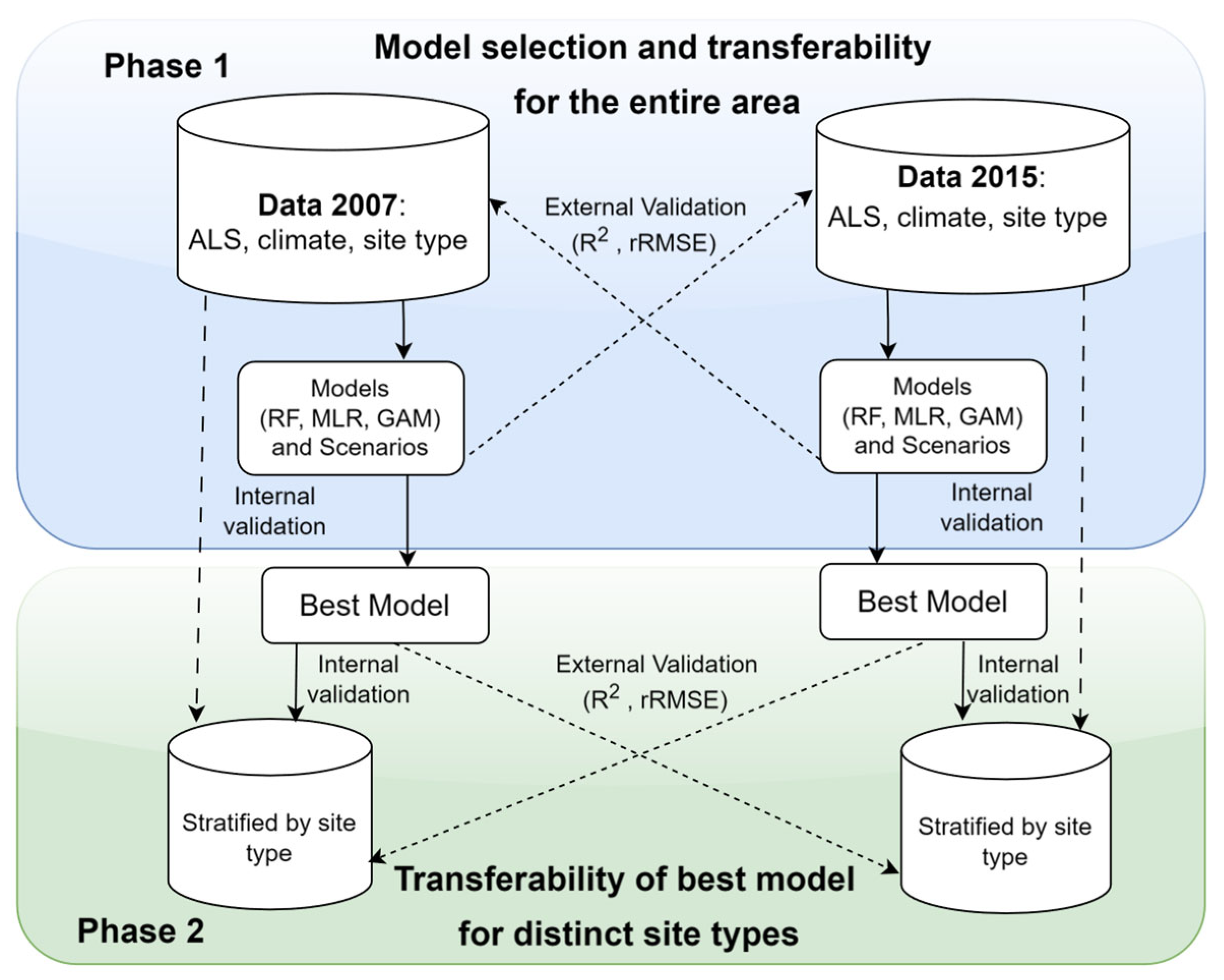
2.3.2. Modelling and Prediction

We tested three modelling methods, including random forest—RF [51], multiple linear regression—MLR, and the generalized additive model—GAM [52,53] to predict GSV. These methods allowed us to strike a balance between model flexibility, as is the case with RF and the GAM, and model interpretability, as is the case with MLR and the GAM. We implemented the GAM using the mgcv package [52,53], via restricted maximum likelihood (REML) to avoid overfitting. The default thin-plate spline function (s) was used for continuous variables as needed. To assess the interaction effects between predictors, both with and without the main effect, the tensor product interaction smooth (ti) or the tensor product smooth (te) functions were applied, respectively. Additionally, the degrees of freedom of these functions were adjusted as necessary to prevent overfitting. Random forest regression was implemented from the ranger package [54]. The default tuning parameters were used, however, setting the number of trees to 2000 to ensure error stabilization and minimize overfitting risks while maintaining computational efficiency. MLR was implemented because of its simplicity and the fact that it has sometimes outperformed or performed equally well as RF or other complex models in biomass and GSV prediction [15,22,32]. All statistical modelling was performed in R [55].
To answer the first research question about the benefits of integrating climate and site factors to improve volume predictions, three scenarios were considered for each period and each modelling approach. These included the most complex models integrating ALS and climate and site factors (sa), the simplest models based solely on ALS-derived variables (sb), and moderately complex models integrating ALS and site type (sc). This approach allowed us to apply an F-test in the case of MLR to verify whether these ancillary variables made significant contributions to GSV prediction. In the modelling workflow, GSV was log-transformed to fulfil data requirements for MLR and GAM. We also iteratively tested the model with competing but equally relevant predictors, as was the case among (zmax, zq85, zq85, zq75, and zq65) or among (MAT, DD.5, and SHM), selecting the best based on Akaike’s Information Criterion (AIC).

2.3.3. Model Validation and Selection

These models were validated internally and externally. A leave-one-out cross-validation (LOOCV) approach, which trains the models on all but one data point and predicts the excluded point using the entire dataset, was applied to internally validate the models. For external validation, we used alternative data that were not included in the model training process. We then evaluated model performance and precision based on the relative root mean square error (rRMSE), the coefficient of determination (R2), and model bias (Table 5). The rRMSE is a measure of how close predicted values are to observed values. It was calculated by dividing the RMSE by the mean of GSV for each modelling period. Bias captures the direction of model consistency from the true value. Comparing these metrics for validated models was the basis for selecting the best method to evaluate model performance across various site types.
A permutation test consisting of 1000 iterations based on the root mean square error (RMSE) was implemented to further cross-validate the models and assess the climate’s contribution to model performance. This permutation compared the full models that included climate and site conditions to a reduced model that excluded one or both of these variables. In each iteration, GSV was randomly sampled for each modelling period. This allowed us to calculate and compare the difference in RMSE between the two sets of models. Finally, we derived the p-value from the proportion of permuted RMSE values that exceeded the observed difference in RMSE. The permutation test was essential, especially for GAMs, which were unnested, making the conventional likelihood ratio test (ANOVA-Chi-square) or AIC test insufficient for comparing and justifying model complexity [56].
Hence, with the entire and site type datasets, model transferability was evaluated by comparing the rRMSE and R2 of externally validated datasets to the corresponding reference values for each modelling scenario. In other words, we tested the stability and robustness of models trained with datasets at time t1 against the datasets at time t2 (forward transferability) and vice versa (backward transferability) by comparing the rRMSE and R2 of externally and internally validated models. As shown in the schematic description of the modelling workflow (Figure 2), in Phase 1, both internal and external validation were employed to select the best model for the entire study area. Internal validation involved evaluating model performance on the training data from 2007 and 2015, while external validation then involved testing the model’s predictive ability on the unseen 2007 and 2015 datasets to assess its overall effectiveness across the entire forest area. In Phase 2, the focus shifted to site types. This approach ensured that the best model was not only robust across the entire study area but also effective when applied to specific environmental contexts.

3. Results

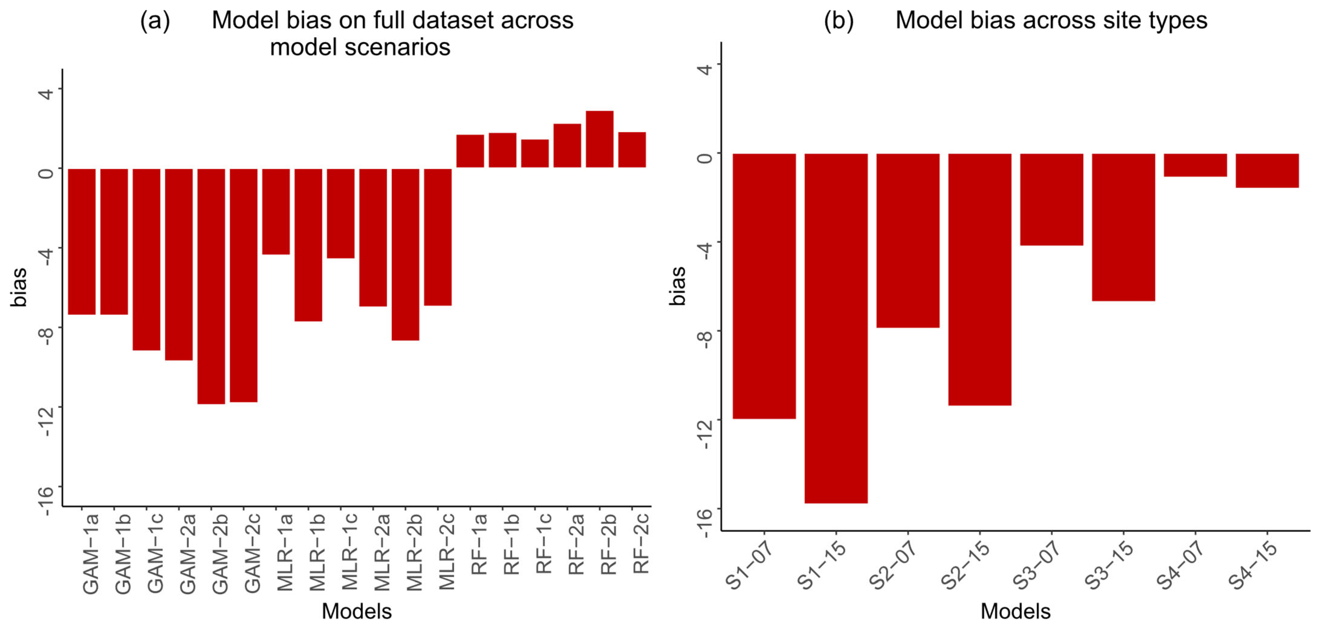
3.1. Model Performance

Figure 3 shows the goodness-of-fit statistics between the modelled GSV and calculations from the field inventory for the three modelling approaches and scenarios in the entire dataset. The coefficient of variability (R2) explained by these models varied from 70% to 58%, decreasing from GAM to RF models, respectively. The R2 value decreased for GAM and MLR, but was nearly constant for RF. Generally, the full models (sa scenario) for MLR (Figure 3a,d) and GAM (Figure 3g,j) consistently explained the most variability. Between the modelling approaches, the full GAM (GAM-2a, Figure 3j) explained 6% and 8% more variability in GSV than MLR and RF, respectively. Similarly, the full MLR model (MLR-1a and MLR-2a) accounted for approximately 6% and 5% more variability in GSV than the model based solely on ALS-derived variables. The difference for RF models was between 2% and 3%, respectively. Additionally, all models were better at predicting lower values of GSV compared to higher values.
Figure 3 also shows that the rRMSE generally decreased with the integration of ancillary data. The rRMSE at t2 was generally lower compared to the rRMSE at t1. Compared to models trained solely on ALS parameters, the rRMSE for the GAM models GAM-1a (Figure 3g) and GAM-2a (Figure 3j) decreased by 4%. Likewise, the MLR models MLR-1a (Figure 3a) and MLR-2a (Figure 3d) showed a decrease of 6% and 5%, respectively. For random forest, the rRMSE either remained unchanged or decreased by 2%.
Model bias for the entire dataset showed a negative trend for GAM and MLR models (Figure 4a). Additionally, GAM and MLR models at time t2 exhibited more bias compared to t1. On the contrary, RF models had a low positive bias, which also increased from t1 to t2. At t2, the GAM-2b and GAM-2c models were even more biased with the exclusion of climatic factors from the model. In the case of MLR, model bias decreased with the integration of site and climatic factors (Figure 4a).
GAM: generalized additive model, MLR: multiple linear regression, RF: random forest. Values “1” and “2” represent models at times t1 (2007) and t2 (2015), respectively. The letters ‘a’, ‘b’, and ‘c’ represent the scenarios ALS + site + climate, ALS only, and ALS + site, respectively. In Figure 4b, S1–S4 refers to the site types. The numbers 07 and 15 refer to the years 2007 and 2015, respectively.
A similar negative trend in model bias for distinct site conditions is also shown in Figure 4b. The figure also shows that model bias was more negative at time t1 compared to t2. Generally, model bias progressively decreases from site type 1 to site type 4.
Table 6 shows the model structure and test statistics for models based on the entire dataset. The table shows that models based only on ALS data had the highest AIC values. In contrast, models that included both climate and site data had the lowest values. The significance of this difference can also be seen from the proportion of permuted RMSEs greater than the RMSE of the original data relative to the number of iterations expressed as p-values. The results show that the comparison between full and reduced models was statistically significant, with p-values in the range 0.001 < p ≤ 0.09, except for the comparison with the reduced MLR model (MLR-2b) at time t2, which showed marginal statistical significance (p-value ~ 0.09).

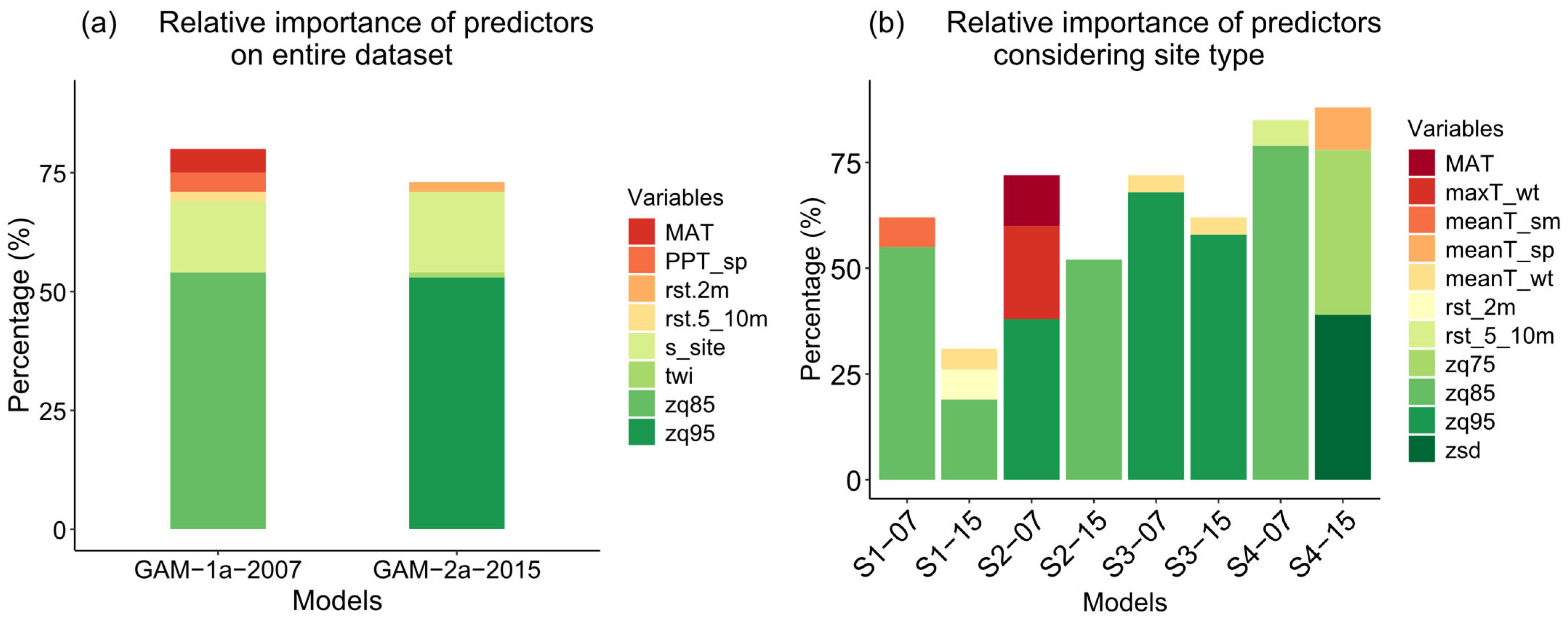
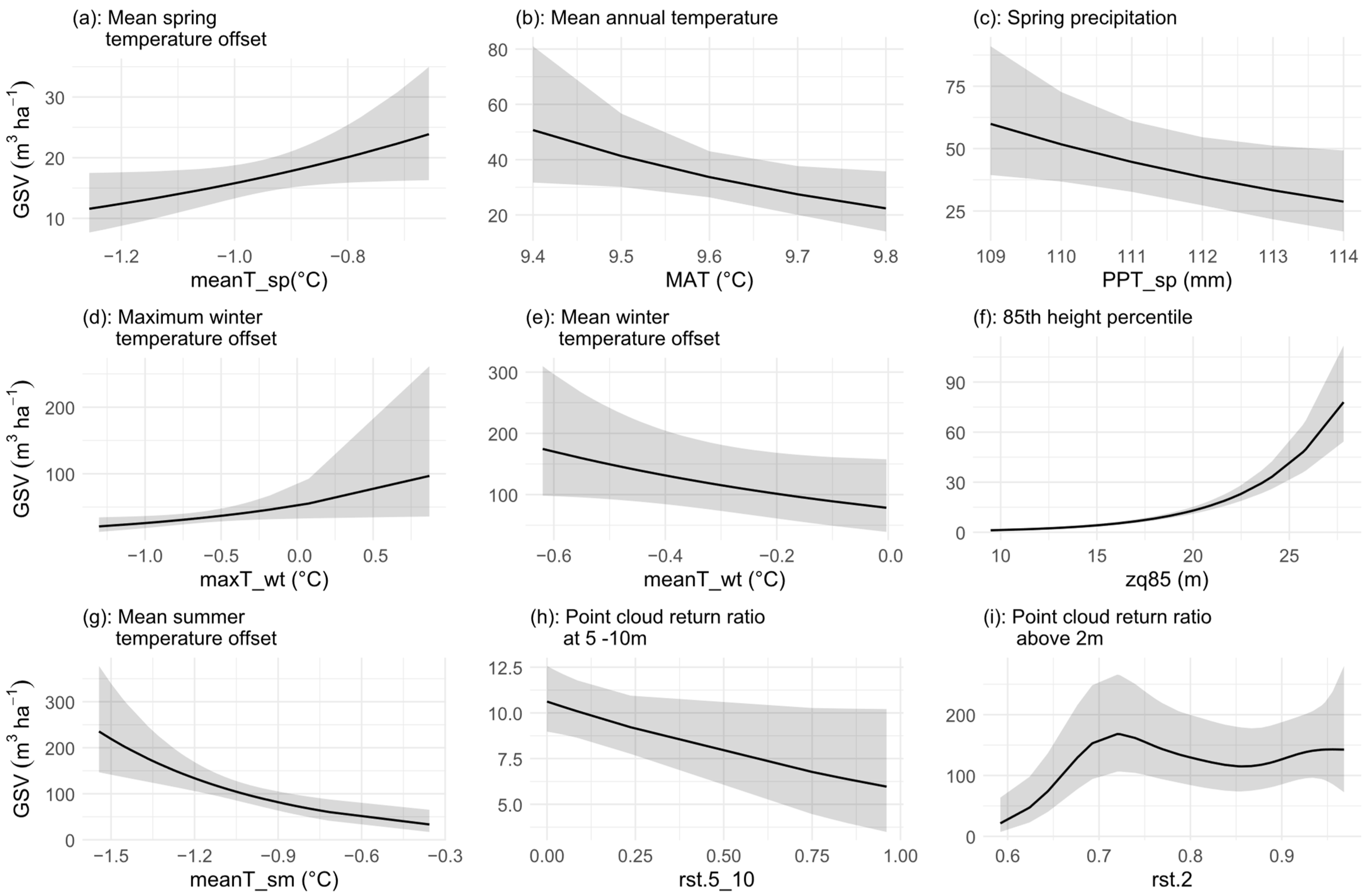
3.2. Variable Importance and Interaction

All three modelling approaches showed that the 85th (zq85) and 95th (zq95) height percentiles were the most important predictors of growth (Figure 5). The full GAM model results showed that these height variables accounted for over 54% of the variability explained by the models. This was followed by site factors, which explained about 17%. Temperature and precipitation and their interaction effects contributed about 9%, while return ratios contributed about 2% (Figure 5a).
See Table 4 and Figure 3 for an explanation of the abbreviations. The figures show the coefficient of variability (R2) explained by each variable based on the training datasets. Green colors in the legend are the ALS height percentiles and site condition, while orange–red colors are the climate variables
Considering distinct site conditions, the contributions of zq85 and zq95 varied between 20% and 75% across the two periods (Figure 5b). Other significant predictors included Mean Annual Temperature (MAT) and maximum temperature in winter (maxT_wt). However, these were only notable at time t1 for site type 2 (s2-07), contributing 12% and 22%, respectively. The mean summer and mean winter temperature offsets contributed about 7% and 4% at sites S1 and S3, respectively. The proportion of ALS returns rst.5_10m, and rst.2m contributed about 6% and 7%, respectively.
The effect of individual predictors on GSV while holding other predictors at their mean values (partial effect) at each site is shown in Figure 6. Overall, GSV gradually decreased with increases in MAT (Figure 6b), meanT_wt (Figure 6e), PPT_sp (Figure 6c), and rst.5_10m (Figure 6h), though with considerable uncertainty. Similarly, GSV also decreased with an increase in mean summer temperature offset (Figure 6g), with less uncertainty, however. On the contrary, zq85, rst.2m, meanT_sp, and maxT_wt positively influenced GSV, with zq85 having the strongest effect. However, the uncertainty associated with meanT_sp and maxT_wt on GSV increases as temperature increases.

3.3. Model Transferability

A comparison of model R2 and rRMSE between internal and external validation on the full datasets for each modelling scenario is presented in Figure 7. The figure shows that across the two modelling periods, the rRMSEs for scenarios integrating only ALS and site factor, irrespective of modelling method, were the most comparable. Additionally, the rRMSE increased as expected; however, there were differences between the modelling approaches. The forward transferability (t1 to t2, Figure 5a) for RF was more comparable to the reference rRMSE than the backward transferability (t2 to t1, Figure 5b). Similarly, the forward transferability for MLR (excluding the transfer scenario s1a_to_s2a), which had an unexpectedly high rRMSE, was more comparable to the reference than the backward transferability. Additionally, the GAM backward transfer for the scenarios s2a_to_s1a and s2b_to_s1b was more stable than their corresponding forward transfer scenarios.
The R2 for the GAM and MLR was generally lower than the reference values. Moreover, the R2 values for all three MLR scenarios were more comparable to the reference values than for GAM scenarios. For example, the difference in R2 for the MLR scenario s1a_to_s2a was approximately 6%, while for GAM, the difference was approximately 12% for the same scenario.
The model transferability between similar site types for the two modelling periods is summarized in Table 7. As expected, the table also shows a general increase in external rRMSEs compared to the reference model. The most comparable rRMSE, with a difference of 10%, was achieved for the forward transferability between site type 4 (S4_07 to S4_15). However, its backward transferability (S4_15 to S4_07) was weak, with an rRMSE difference of approximately 30%. The difference in R2 for transferability between site type 2 (S2_07 to S2_15) was 3% compared to 18% between site type 1 (S1_15 to S1_07). In general, the R2 for externally validated models decreased compared to the reference values, except between site type 3 (S3_07 to S3_15) and site type 4 (S4_07 to S4_15), which were higher than their reference values.

4. Discussion

This study investigated the interaction of vegetation structure derived from ALS data with climate and site-specific conditions over two time periods (2007 and 2015) to improve GSV prediction and evaluate its temporal transferability. We approached this research problem by testing models with varying complexity and considering the uniqueness of different sites. Our key findings suggest that although ALS-derived parameters alone provide a baseline for volume prediction, climate and site-specific data can significantly enhance model performance and should not be overlooked. The improvement in our results was characterized by an increase in R2 by 6% and 8% and a decrease in rRMSE by 6% and 12%, respectively, for the two modelling periods (Figure 3). The consistency of model performance was further confirmed by a statistically significant RMSE-based permutation test, which showed p-values in the range 0.09 < p ≤ 0.001 (Table 6). In other words, we found evidence that the integration of climate and site conditions into ALS data can improve GSV estimation. However, the direct contribution of climate alone to GSV prediction was marginal. Hence, these results confirmed our claim that the simpler model based solely on ALS predictors was insufficient for capturing the complexities of GSV dynamics.

4.1. Model Performance and Selection

Comparing the results of the internally validated models on the full dataset for the different modelling approaches, we found that the GAM consistently outperformed MLR and RF in all three modelling scenarios. This was evident from its relatively low rRMSE and high R2 compared to MLR and RF (Figure 3). However, the GAM was the most biased and generally underpredicted volume compared to MLR (Figure 4). The bias in the GAM and MLR compared to the sample mean varied from 12% to 15%, compared to 6% to 12%, respectively. Random forest was the least biased, slightly overpredicting GSV (Figure 4). However, its rRMSE and R2 remained nearly constant with or without the integration of climate and site type data (Figure 5), suggesting that the influence of these ancillary variables in the RF model was overshadowed by ALS-derived variables. While previous studies comparing GSV predictions based solely on ALS-derived variables found very marginal differences between modelling approaches [22,32], our GAM results showed that the difference was statistically significant, with p-values generally ≤0.023 with the integration of environmental variables (Table 5). This finding explains our preference for GAM over RF and MLR to further evaluate the role of climate and environmental conditions on GSV prediction in each of the four unique site types of the study area. Our model results at this scale showed significant variability in volume, which differed between site types and modelling periods, emphasizing not only the importance of spatial resolution but also site quality in GSV prediction [5,8].

4.2. Model Validation and Transferability

Our results showed that the different transfer scenarios and modelling approaches responded differently to model transfer. In general, the best transferable scenario was between models integrating site type and ALS-derived variables (sc), possibly because site type conditions are generally more stable compared to dynamic climatic conditions. Random forest was the most stable to temporal transferability in both directions, especially for the modelling scenario that integrated climate and site type into ALS data. RF consistently maintained a relatively low rRMSE (Figure 7a,b) and higher R2 values (Figure 7c,d) on external validation, highlighting its flexibility in integrating multi-source data. This result contrasts with those of Zhao et al. [15], who assessed transferability exclusively on ALS-based models and reported that RF had a general tendency to overfit, compared to MLR.
GAMs showed a relatively high potential for temporal transferability compared to MLR. This was shown by the fact that GAM performed relatively well in both forward and backward transferability for all scenarios (Figure 7). In contrast, only backward transferability was optimal for MLR, indicating that there might be potential challenges in adapting the model across different temporal datasets. The limitation of MLR could be seen from the fact that the difference between the internal and external rRMSE for GAM ranged from 10% to 70%, but could be up to 400% higher for MLR. The performance of GAM highlights the importance of capturing non-linear relationships, especially for models intended to test temporal transferability in the face of climate change, noted similarly by [57].
Models based on unique site conditions (Table 7) generally captured the inherent variability in GSV. Although the difference between internal and external R2 was small and varied from 2% to 18%, these models did not significantly improve model accuracy, considering that the difference in rRMSE range (10% to 45%) was comparable to models trained on the entire dataset. Nevertheless, site-specific models were valuable for understanding ALS–climate interaction, a scenario we could not model using the entire dataset without considering site type. In this regard, Figure 5b suggests that although the overall role of microclimate may be weak across the area, its influence is highly specific to certain sites and has significant potential to enhance the GSV model, especially with a much higher resolution dataset.
Our justification for using both R2 and rRMSE to evaluate model transferability was to strike a balance between model fit and accuracy. Our results show that these metrics are not equally comparable in every scenario. For instance, in the MLR scenario s1a_to_s2a (Figure 7c), the R2 from external validation was nearly the same as the internal R2, indicating that the model captured the GSV trend. However, the high rRMSE (Figure 7a) suggested poor overall agreement with the reference model despite the strong R2. In comparison with the GAM and MLR transferability scenarios s1c_to_s2c, the external R2 and rRMSE were high and low, respectively, and very comparable to the reference (Figure 7a,c), which is an indication of better transferability. Thus, while rRMSE is a better indicator of model accuracy, R2 reflects the model’s explanatory power, making it a complementary metric to rRMSE. In comparison with existing studies that have evaluated model transferability in different ecological settings [15,34,57,58], this research provides insights into the robustness of such models amidst simultaneous changes in environmental conditions and vegetation structure.

4.3. Variable Importance

We found that the 85th and 95th ALS height percentiles were the most important predictors for the modelling periods, explaining up to 75% of the variability in GSV. These findings are broadly consistent with prior research that highlights the importance of ALS data in GSV and biomass prediction [15,28,29,31,32,59]. Less important but equally significant ALS variables in all models included the proportion of ALS returns rst.2m and rst_5-10. The contribution of MAT and PPT_sp (Figure 5a) was marginal, in agreement with [3], and also showed an inconsistent interaction effect on GSV across time, highlighting the complex role of climate. In general, forest climate variables were more important in models based on unique site types than in general models for the entire study area

4.4. Limitations and Future Directions

Despite promising results, important limitations linked to data quality must be acknowledged. First, the spatial inconsistency between ALS and climate and between ALS datasets may have introduced uncertainties that decreased the accuracy of the model [15,39]. Second, the temporal gap in GSV measurements for 2007, which we filled by linear interpolating from field-calculated measurements in 2005 and 2015, assumed that the rate of GSV increase is constant. In reality, this assumption will rarely be the case because the processes influencing GSV are dynamic and inconsistent and tend to be sensitive to lags, delays, and seasonal variability, which are predominantly climate-dependent [3]. As such, the natural variability in GSV in 2007 may have been lost in our estimations, introducing some bias, in addition to bias related to the relatively small sample size of our dataset. These limitations may further explain why attempts to test ALS + climate only as a possible scenario in our modelling workflow were unsuccessful for the GAM when we excluded site type from models trained with the entire dataset.
Future research may expand on the temporal scope of this study beyond two time stamps. This would allow for a more thorough assessment of the model’s robustness and its practical application, providing better insights into growth dynamics compared to bitemporal analysis [15]. Lastly, it must be noted that the combined influence of climate and vegetation structure on GSV for small-scale studies is complex. Age or species-based stratification approaches using high-resolution micro-climate data should be considered to provide a better understanding of the role of microclimate. Additionally, complementary studies from process-based models adapted to capture the effect of temporal shifts in temperature and precipitation on ecological processes could reveal how changes in environmental conditions might affect model transferability.

5. Conclusions

This research evaluates the potential of integrating microclimate, site-specific information and ALS data into GAM, ML, and RF models, under different modelling scenarios of varying complexity to improve the accuracy of GSV prediction and evaluate temporal transferability between 2007 (t1) and 2015 (t2). We showed this with an RMSE-based permutation test (p ≤ 0.023), which confirmed that climate significantly influenced GSV prediction when integrated with ALS data. We also noted that the direct contribution of climate to model performance was marginal on a broad scale. However, its role in GSV prediction and temporal transferability seems stronger in homogeneous sites. In general, RF was the most stable in both the forward (t1→t2) and backward (t2→t1) directions, for the modelling scenario integrating ALS with climate and site type, unlike the GAM, which was more stable in the backward direction. Furthermore, we noted that the interaction between vegetation structure and climate variability on GSV is complex and needs further investigation, possibly expanding the temporal scope of this research while considering environmental gradients to further confirm model transferability for long-term monitoring and management. This study provides a multidisciplinary framework for assessing the reliability of GSV models and addresses a critical gap in forest monitoring.

Author Contributions

Conceptualization, E.T., K.S., Y.E., and W.T.; methodology, E.T., K.S., M.M., and Y.E.; data curation, M.M., Y.E., and E.T.; formal analysis, M.M., E.T., and W.T.; visualization, E.T., M.M., and W.T.; writing—original draft preparation, E.T., M.M., W.T., and Y.E.; writing—review and editing, K.S., M.M., W.T., and Y.E.; supervision, K.S. and Y.E. All authors have read and agreed to the published version of the manuscript.

Funding

This research was internally funded by IDEAS NCBR Sp. z o.o., Poland and by project financed by the National Center for Research and Development as part of the 5th competition for Poland-Türkiye Cooperation, contract number: 1/12/2023 r: POLTUR5/2022/45/SILVA_NYMPHA/2023.

Data Availability Statement

The research data are available upon request and can be obtained with the permission of the Forest Research Institute (IBL), Poland.

Acknowledgments

We would like to thank the Forest Research Institute (IBL), Poland, for providing the ALS and forest inventory data.

Conflicts of Interest

The authors declare no conflicts of interest.

References

  1. Krejza, J.; Světlík, J.; Bednář, P. Allometric Relationship and Biomass Expansion Factors (BEFs) for above- and below-Ground Biomass Prediction and Stem Volume Estimation for Ash (Fraxinus excelsior L.) and Oak (Quercus robur L.). Trees Struct. Funct. 2017, 31, 1303–1316. [Google Scholar] [CrossRef]
  2. Kurz, W.A.; Dymond, C.C.; White, T.M.; Stinson, G.; Shaw, C.H.; Rampley, G.J.; Smyth, C.; Simpson, B.N.; Neilson, E.T.; Trofymow, J.A.; et al. CBM-CFS3: A Model of Carbon-Dynamics in Forestry and Land-Use Change Implementing IPCC Standards. Ecol. Model. 2009, 220, 480–504. [Google Scholar] [CrossRef]
  3. Anderson-Teixeira, K.J.; Herrmann, V.; Rollinson, C.R.; Gonzalez, B.; Gonzalez-Akre, E.B.; Pederson, N.; Alexander, M.R.; Allen, C.D.; Alfaro-Sánchez, R.; Awada, T.; et al. Joint Effects of Climate, Tree Size, and Year on Annual Tree Growth Derived from Tree-Ring Records of Ten Globally Distributed Forests. Glob. Change Biol. 2022, 28, 245–266. [Google Scholar] [CrossRef] [PubMed]
  4. Cienciala, E.; Russ, R.; Šantrůčková, H.; Altman, J.; Kopáček, J.; Hůnová, I.; Štěpánek, P.; Oulehle, F.; Tumajer, J.; Ståhl, G. Discerning Environmental Factors Affecting Current Tree Growth in Central Europe. Sci. Total Environ. 2016, 573, 541–554. [Google Scholar] [CrossRef]
  5. Larson, J.; Vigren, C.; Wallerman, J.; Ågren, A.M.; Appiah Mensah, A.; Laudon, H. Tree Growth Potential and Its Relationship with Soil Moisture Conditions across a Heterogeneous Boreal Forest Landscape. Sci. Rep. 2024, 14, 10611. [Google Scholar] [CrossRef]
  6. Pretzsch, H.; Biber, P.; Schütze, G.; Uhl, E.; Rötzer, T. Forest Stand Growth Dynamics in Central Europe Have Accelerated since 1870. Nat. Commun. 2014, 5, 4967. [Google Scholar] [CrossRef]
  7. Schut, A.G.T.; Wardell-Johnson, G.W.; Yates, C.J.; Keppel, G.; Baran, I.; Franklin, S.E.; Hopper, S.D.; Van Niel, K.P.; Mucina, L.; Byrne, M. Rapid Characterisation of Vegetation Structure to Predict Refugia and Climate Change Impacts across a Global Biodiversity Hotspot. PLoS ONE 2014, 9, e82778. [Google Scholar] [CrossRef]
  8. Unterholzner, L.; Stolz, J.; van der Maaten-Theunissen, M.; Liepe, K.; van der Maaten, E. Site Conditions Rather than Provenance Drive Tree Growth, Climate Sensitivity and Drought Responses in European Beech in Germany. For. Ecol. Manag. 2024, 572, 122308. [Google Scholar] [CrossRef]
  9. Gril, E.; Laslier, M.; Gallet-Moron, E.; Durrieu, S.; Spicher, F.; Le Roux, V.; Brasseur, B.; Haesen, S.; Van Meerbeek, K.; Decocq, G.; et al. Using Airborne LiDAR to Map Forest Microclimate Temperature Buffering or Amplification. Remote Sens. Environ. 2023, 298, 113820. [Google Scholar] [CrossRef]
  10. Zellweger, F.; De Frenne, P.; Lenoir, J.; Vangansbeke, P.; Verheyen, K.; Bernhardt-Römermann, M.; Baeten, L.; Hédl, R.; Berki, I.; Brunet, J.; et al. Forest Microclimate Dynamics Drive Plant Responses to Warming. Science (1979) 2020, 368, 772–775. [Google Scholar] [CrossRef]
  11. Beland, M.; Parker, G.; Sparrow, B.; Harding, D.; Chasmer, L.; Phinn, S.; Antonarakis, A.; Strahler, A. On Promoting the Use of Lidar Systems in Forest Ecosystem Research. For. Ecol. Manag. 2019, 450, 117484. [Google Scholar] [CrossRef]
  12. Lefsky, M.A.; Cohen, W.B.; Parker, G.G.; Harding, D.J. Lidar Remote Sensing for Ecosystem Studies. Bioscience 2002, 52, 19–30. [Google Scholar] [CrossRef]
  13. Bouvier, M.; Durrieu, S.; Fournier, R.A.; Renaud, J.P. Generalizing Predictive Models of Forest Inventory Attributes Using an Area-Based Approach with Airborne LiDAR Data. Remote Sens. Environ. 2015, 156, 322–334. [Google Scholar] [CrossRef]
  14. Marinelli, D.; Paris, C.; Bruzzone, L. A Novel Approach to 3-D Change Detection in Multitemporal LiDAR Data Acquired in Forest Areas. IEEE Trans. Geosci. Remote Sens. 2018, 56, 3030–3046. [Google Scholar] [CrossRef]
  15. Zhao, K.; Suarez, J.C.; Garcia, M.; Hu, T.; Wang, C.; Londo, A. Utility of Multitemporal Lidar for Forest and Carbon Monitoring: Tree Growth, Biomass Dynamics, and Carbon Flux. Remote Sens. Environ. 2018, 204, 883–897. [Google Scholar] [CrossRef]
  16. Yu, X.; Hyyppä, J.; Kaartinen, H.; Maltamo, M.; Hyyppä, H. Obtaining Plotwise Mean Height and Volume Growth in Boreal Forests Using Multi-Temporal Laser Surveys and Various Change Detection Techniques. Int. J. Remote Sens. 2008, 29, 1367–1386. [Google Scholar] [CrossRef]
  17. Moudrý, V.; Cord, A.F.; Gábor, L.; Laurin, G.V.; Barták, V.; Gdulová, K.; Malavasi, M.; Rocchini, D.; Stereńczak, K.; Prošek, J.; et al. Vegetation Structure Derived from Airborne Laser Scanning to Assess Species Distribution and Habitat Suitability: The Way Forward. Divers. Distrib. 2023, 29, 39–50. [Google Scholar] [CrossRef]
  18. Knapp, N.; Fischer, R.; Cazcarra-Bes, V.; Huth, A. Structure Metrics to Generalize Biomass Estimation from Lidar across Forest Types from Different Continents. Remote Sens. Environ. 2020, 237, 111597. [Google Scholar] [CrossRef]
  19. Hauglin, M.; Rahlf, J.; Schumacher, J.; Astrup, R.; Breidenbach, J. Large Scale Mapping of Forest Attributes Using Heterogeneous Sets of Airborne Laser Scanning and National Forest Inventory Data. For. Ecosyst. 2021, 8, 65. [Google Scholar] [CrossRef]
  20. Ma, Q.; Su, Y.; Tao, S.; Guo, Q. Quantifying Individual Tree Growth and Tree Competition Using Bi-Temporal Airborne Laser Scanning Data: A Case Study in the Sierra Nevada Mountains, California. Int. J. Digit. Earth 2018, 11, 485–503. [Google Scholar] [CrossRef]
  21. Knapp, N.; Fischer, R.; Huth, A. Linking Lidar and Forest Modeling to Assess Biomass Estimation across Scales and Disturbance States. Remote Sens. Environ. 2018, 205, 199–209. [Google Scholar] [CrossRef]
  22. Parkitna, K.; Krok, G.; Miścicki, S.; Ukalski, K.; Lisańczuk, M.; Mitelsztedt, K.; Magnussen, S.; Markiewicz, A.; Stereńczak, K. Modelling Growing Stock Volume of Forest Stands with Various ALS Area-Based Approaches. Forestry 2021, 94, 630–650. [Google Scholar] [CrossRef]
  23. Tompalski, P.; Coops, N.C.; White, J.C.; Goodbody, T.R.H.; Hennigar, C.R.; Wulder, M.A.; Socha, J.; Woods, M.E. Estimating Changes in Forest Attributes and Enhancing Growth Projections: A Review of Existing Approaches and Future Directions Using Airborne 3D Point Cloud Data. Curr. For. Rep. 2021, 7, 1–24. [Google Scholar] [CrossRef]
  24. White, J.; Wulder, M.; Varhola, A.; Vastaranta, M.; Coops, N.; Cook, B.D.; Pitt, D.; Woods, M. A Best Practices Guide for Generating Forest Inventory Attributes from Airborne Laser Scanning Data Using an Area-Based Approach; Natural Resources Canada: Victoria, BC, Canada, 2013. [Google Scholar]
  25. Penner, M.; Pitt, D.G.; Woods, M.E. Parametric vs. Nonparametric LiDAR Models for Operational Forest Inventory in Boreal Ontario. Can. J. Remote Sens. 2013, 39, 426–443. [Google Scholar] [CrossRef]
  26. Bollandsås, O.M.; Ene, L.T.; Gobakken, T.; Næsset, E. Estimation of Biomass Change in Montane Forests in Norway along a 1200 Km Latitudinal Gradient Using Airborne Laser Scanning: A Comparison of Direct and Indirect Prediction of Change under a Model-Based Inferential Approach. Scand. J. For. Res. 2018, 33, 155–165. [Google Scholar] [CrossRef]
  27. Cao, L.; Coops, N.C.; Innes, J.L.; Sheppard, S.R.J.; Fu, L.; Ruan, H.; She, G. Estimation of Forest Biomass Dynamics in Subtropical Forests Using Multi-Temporal Airborne LiDAR Data. Remote Sens. Environ. 2016, 178, 158–171. [Google Scholar] [CrossRef]
  28. Dalponte, M.; Jucker, T.; Liu, S.; Frizzera, L.; Gianelle, D. Characterizing Forest Carbon Dynamics Using Multi-Temporal Lidar Data. Remote Sens. Environ. 2019, 224, 412–420. [Google Scholar] [CrossRef]
  29. McRoberts, R.E.; Næsset, E.; Gobakken, T.; Bollandsås, O.M. Indirect and Direct Estimation of Forest Biomass Change Using Forest Inventory and Airborne Laser Scanning Data. Remote Sens. Environ. 2015, 164, 36–42. [Google Scholar] [CrossRef]
  30. Tompalski, P.; Rakofsky, J.; Coops, N.C.; White, J.C.; Graham, A.N.V.; Rosychuk, K. Challenges of Multi-Temporal and Multi-Sensor Forest Growth Analyses in a Highly Disturbed Boreal Mixedwood Forests. Remote Sens. 2019, 11, 2102. [Google Scholar] [CrossRef]
  31. Coops, N.C.; Tompalski, P.; Goodbody, T.R.H.; Queinnec, M.; Luther, J.E.; Bolton, D.K.; White, J.C.; Wulder, M.A.; van Lier, O.R.; Hermosilla, T. Modelling Lidar-Derived Estimates of Forest Attributes over Space and Time: A Review of Approaches and Future Trends. Remote Sens. Environ. 2021, 260, 112477. [Google Scholar] [CrossRef]
  32. Hawryło, P.; Francini, S.; Chirici, G.; Giannetti, F.; Parkitna, K.; Krok, G.; Mitelsztedt, K.; Lisańczuk, M.; Stereńczak, K.; Ciesielski, M.; et al. The Use of Remotely Sensed Data and Polish NFI Plots for Prediction of Growing Stock Volume Using Different Predictive Methods. Remote Sens. 2020, 12, 3331. [Google Scholar] [CrossRef]
  33. Wu, Y.; Mao, Z.; Guo, L.; Li, C.; Deng, L. Forest Volume Estimation Method Based on Allometric Growth Model and Multisource Remote Sensing Data. IEEE J. Sel. Top. Appl. Earth Obs. Remote Sens. 2023, 16, 8900–8912. [Google Scholar] [CrossRef]
  34. Eastburn, J.F.; Campbell, M.J.; Dennison, P.E.; Anderegg, W.R.; Barrett, K.J.; Fekety, P.A.; Flake, S.W.; Huffman, D.W.; Kannenberg, S.A.; Kerr, K.L.; et al. Ecological and Climatic Transferability of Airborne Lidar-Driven Aboveground Biomass Models in Piñon-Juniper Woodlands. GISci. Remote Sens. 2024, 61, 2363577. [Google Scholar] [CrossRef]
  35. Hlásny, T.; Trombik, J.; Bošeľa, M.; Merganič, J.; Marušák, R.; Šebeň, V.; Štěpánek, P.; Kubišta, J.; Trnka, M. Climatic Drivers of Forest Productivity in Central Europe. Agric. For. Meteorol. 2017, 234–235, 258–273. [Google Scholar] [CrossRef]
  36. Charru, M.; Seynave, I.; Hervé, J.C.; Bertrand, R.; Bontemps, J.D. Recent Growth Changes in Western European Forests Are Driven by Climate Warming and Structured across Tree Species Climatic Habitats. Ann. For. Sci. 2017, 74, 33. [Google Scholar] [CrossRef]
  37. Haesen, S.; Lembrechts, J.J.; De Frenne, P.; Lenoir, J.; Aalto, J.; Ashcroft, M.B.; Kopecký, M.; Luoto, M.; Maclean, I.; Nijs, I.; et al. ForestTemp—Sub-Canopy Microclimate Temperatures of European Forests. Glob. Change Biol. 2021, 27, 6307–6319. [Google Scholar] [CrossRef]
  38. Haesen, S.; Lenoir, J.; Gril, E.; De Frenne, P.; Lembrechts, J.J.; Kopecký, M.; Macek, M.; Man, M.; Wild, J.; Van Meerbeek, K. Microclimate Reveals the True Thermal Niche of Forest Plant Species. Ecol. Lett. 2023, 26, 2043–2055. [Google Scholar] [CrossRef]
  39. Yates, K.L.; Bouchet, P.J.; Caley, M.J.; Mengersen, K.; Randin, C.F.; Parnell, S.; Fielding, A.H.; Bamford, A.J.; Ban, S.; Barbosa, A.M.; et al. Outstanding Challenges in the Transferability of Ecological Models. Trends Ecol. Evol. 2018, 33, 790–802. [Google Scholar] [CrossRef]
  40. Moreno-Arzate, C.N.; Martínez-Meyer, E. A Retrospective Approach for Evaluating Ecological Niche Modeling Transferability over Time: The Case of Mexican Endemic Rodents. PeerJ 2024, 12, e18414. [Google Scholar] [CrossRef]
  41. Stereńczak, K.; Lisańczuk, M.; Parkitna, K.; Mitelsztedt, K.; Mroczek, P.; Miścicki, S. The Influence of Number and Size of Sample Plots on Modelling Growing Stock Volume Based on Airborne Laser Scanning. Drewno 2018, 61, 5–22. [Google Scholar] [CrossRef]
  42. Bruchwald, A.; Rymer-Dudzinska, T.; Dudek, A.; Michalak, K.; Wróblewski, L.; Zasada, M. Wzory Empiryczne Do Okreslania Wysokosci i Piersnicowej Liczby Kształtu Grubizny Drzewa (Empirical Formulae for Defining Height and Dbh Shape FIgure of Thick Wood). Sylwan 2000, 144, 5–14. (In Polish) [Google Scholar]
  43. Bruchwald, A.; Miscicki, S.; Dmyterko, E.; Sterenczak, K. Ocena Dokładnosci Obreębowej Metody Inwentaryzacji Lasu Opartej Nalosowaniu Warstwowym (Assessment of the Accuracy of the Forest District Inventory Method Based on the Stratified Sampling). Sylwan 2017, 161, 909–916. (In Polish) [Google Scholar]
  44. White, J.C.; Coops, N.C.; Wulder, M.A.; Vastaranta, M.; Hilker, T.; Tompalski, P. Remote Sensing Technologies for Enhancing Forest Inventories: A Review. Can. J. Remote Sens. 2016, 42, 619–641. [Google Scholar] [CrossRef]
  45. Sparks, A.M.; Smith, A.M.S. Accuracy of a LiDAR-Based Individual Tree Detection and Attribute Measurement Algorithm Developed to Inform Forest Products Supply Chain and Resource Management. Forests 2021, 13, 3. [Google Scholar] [CrossRef]
  46. Strunk, J.L.; McGaughey, R.J. Stand Validation of Lidar Forest Inventory Modeling for a Managed Southern Pine Forest. Can. J. For. Res. 2023, 53, 71–89. [Google Scholar] [CrossRef]
  47. Roussel, J.R.; Auty, D.; Coops, N.C.; Tompalski, P.; Goodbody, T.R.H.; Meador, A.S.; Bourdon, J.F.; de Boissieu, F.; Achim, A. LidR: An R Package for Analysis of Airborne Laser Scanning (ALS) Data. Remote Sens. Environ. 2020, 251, 112061. [Google Scholar] [CrossRef]
  48. Böhner, J.; Selige, T. Spatial prediction of soil attributes using terrain analysis and climate regionalisation. Göttinger Geographische Abhandlungen 2006, 115, 13–28. [Google Scholar]
  49. Conrad, O.; Bechtel, B.; Bock, M.; Dietrich, H.; Fischer, E.; Gerlitz, L.; Wehberg, J.; Wichmann, V.; Böhner, J. System for Automated Geoscientific Analyses (SAGA) v. 2.1.4. Geosci. Model. Dev. 2015, 8, 1991–2007. [Google Scholar] [CrossRef]
  50. Marchi, M.; Castellanos-Acuña, D.; Hamann, A.; Wang, T.; Ray, D.; Menzel, A. ClimateEU, Scale-Free Climate Normals, Historical Time Series, and Future Projections for Europe. Sci. Data 2020, 7, 428. [Google Scholar] [CrossRef]
  51. Breiman, L. Random Forest. Mach. Learn. 2001, 45, 5–32. [Google Scholar] [CrossRef]
  52. Wood, S.N. Generalized Additive Models: An Introduction with R, Second Edition, 2nd ed.; Chapman and Hall/CRC: New York, NY, USA, 2017; ISBN 9781315370279. [Google Scholar]
  53. Zuur, A.F.; Ieno, E.N.; Walker, N.; Saveliev, A.A.; Smith, G.M. Mixed Effects Models and Extensions in Ecology with R; Springer: New York, NY, USA, 2009; ISBN 978-0-387-87457-9. [Google Scholar]
  54. Wright, M.N.; Ziegler, A. Ranger: A Fast Implementation of Random Forests for High Dimensional Data in C++ and R. J. Stat. Softw. 2017, 77, 1–17. [Google Scholar] [CrossRef]
  55. R Core Team. R: A Language and Environment for Statistical Computing; R Foundation for Statistical Computing: Vienna, Austria, 2023. [Google Scholar]
  56. Hastie, T.J.; Tibshirani, R.J. Generalized Additive Models, 1st ed.; Routledge: New York, NY, USA, 2017; ISBN 9780203753781. [Google Scholar]
  57. Araujo, M.; Pearson, R.; Thuiller, W.; Erhard, M. Validation of Species-Climate Impact Models under Climate Change. Glob. Change Biol. 2005, 11, 1504–1513. [Google Scholar] [CrossRef]
  58. Dobrowski, S.Z.; Thorne, J.H.; Greenberg, J.A.; Safford, H.D.; Mynsberge, A.R.; Crimmins, S.M.; Swanson, A.K. Modeling Plant Ranges over 75 Years of Climate Change in California, USA: Temporal Transferability and Species Traits. Ecol. Monogr. 2011, 81, 241–257. [Google Scholar] [CrossRef]
  59. García, M.; Riaño, D.; Chuvieco, E.; Danson, F.M. Estimating Biomass Carbon Stocks for a Mediterranean Forest in Central Spain Using LiDAR Height and Intensity Data. Remote Sens. Environ. 2010, 114, 816–830. [Google Scholar] [CrossRef]
Figure 1. Location of the study area (red rectangle on map insert) and forest and sample plot spatial cover.
Forests 16 00815 g001
Figure 2. Schematic description of the modelling workflow. Modelling was implemented in 2 phases. In Phase 1, the 3 modelling approaches were evaluated for performance and model transferability using the full dataset. In Phase 2, the best model was selected and evaluated for model transferability in distinct sites.
Forests 16 00815 g002
Figure 3. Comparison of observed vs. predicted growing stock volume (GSV) relationships of goodness of fit across modelling approaches and scenarios. GAM: generalized additive model, MLR: multiple linear regression, RF: random forest. (ac) MLR at time t1 (2007), compared to (df) MLR at time t2 (2015). (gi) GAM at t1 comapred to (jl) GAM at t2. (mo) RF at t1 compared to (pr) RF at t2. Model performance metrics (R², rRMSE) demonstrate superior accuracy when including site and climate data (e.g., GAM-1a (g) and GAM-2a (j)) compared to ALS-only models (h,k). Best overall fit ((j), R2 = 0.70, rRMSE 0.66), capturing non-linear trends. The numbers ‘1’ and ‘2’ in the plot title represent the modelling period 2007 and 2015, respectively. The letters ‘a’, ‘b’ and ‘c’ in the plot title symbolize the model scenarios ALS + climate and site factors, ALS only, and ALS + site type, respectively. The first three columns to the left compare models trained with 2007 (left panels). The last three columns compare models trained with the 2015 dataset.
Forests 16 00815 g003
Figure 4. Comparison of model bias: (a) based on the full dataset for different modelling approaches and model scenarios, and (b) between site types, based on the GAM.
Forests 16 00815 g004
Figure 5. Relative importance of GAM-based predictors. (a) data from all plots, (b) site-specific plots.
Forests 16 00815 g005
Figure 6. Partial effects of key predictors on growing stock volume (GSV): (a) mean spring temperature offset, (b) mean annual temperature, (c) spring precipitation, (d) maximum winter temperature offset, (e) mean winter temperature offset, (f) mean summer temperature offset, (g) 85th height percentile, (h) point cloud return ratio at 5–10 m, and (i) point cloud return ratio above 2 m from ALS data. Solid lines show predicted effects, with shading representing 95% confidence intervals. Notable patterns include decreasing GSV at temperature extremes and positive relationships with structural metrics (f,g). All temperature values are in °C. Note. The range of volume growth is different from the full dataset to improve visualization.
Forests 16 00815 g006
Figure 7. Comparison of model transferability between 2007 (t1) and 2015 (t2) datasets and modelling approaches. (a) Relative root mean square error (rRMSE) for models trained on t1 and tested on t2 (forward transferability) versus internal leave-one-out cross-validation (LOOCV) rRMSE at t1. (b) rRMSE for models trained on t2 and tested on t1 (backward transferability) versus LOOCV rRMSE at t2. (c,d) Corresponding R2 values for forward and backward transferability. Models include ALS-only (b), ALS + site type (c), and ALS + site type + climate. The letters “a”, “b”, and “c” in the legend represent these model scenarios, respectively, while numbers 1 and 2 represent the modelling period. Thus, the letters and numbers together describe the transfer scenario.
Forests 16 00815 g007
Table 1. Summary of repeated plot inventory of tree height, diameter at breast height (DBH). and growing stock volume per hectare.
Plot SummaryMinimumMaximumMeanStandard Deviation
2005 (# trees = 763)
Mean height [m]54022.116.5
Mean DBH [cm]7.575.726.5112.15
GSV [m3/ha]0.4513.854.6382.67
2007 *
Mean tree height [m]6.340.7722.776.43
Mean DBH [cm]8.3276.5827.712.07
GSV [m3/ha]0.56539.7260.0186.06
2015 (# trees = 763)
Mean tree height [m]11.544.125.35.89
Mean DBH [cm]10.780.1229.5612.65
GSV [m3/ha]1.2643.482.67100.68
* Inventory parameter for 2007 was estimated using Equation (2). Note the number of plots with repeated measurements = 181. The number of trees with repeated measurements = 763. Plots or trees with incomplete measurements, such as missing tree heights, were not considered.
Table 2. Summary of ALS data characteristics.
ALS1 (2007), t1ALS2 (2015), t2
ScannerTopoSys GmbH FALCON IIRiegl LMSQ680i
Flight height700 m550 m
Data recordingMay 2007August 2015
Scanning angle±7.1°60°
Scan frequency83 kHz360 kHz
Average point density7 points/m210 points/m2
Area covered90.68 km2225.65 km2
SeasonLeaf onLeaf on
Table 3. Summary description of site types.
Site CodeDescriptionSoil Characteristics
S1Pine-dominatedSandy soils
S2Broadleaf (oak, ash, maple, and birch)Rich fertile soils
S3Mixed broadleaf (oak, ash, and maple)Soils of varying fertility
S4Alder and willow-dominatedWet-to-water-logged soils
Table 4. Relevant explanatory variables used for model training.
MetricsAbbreviationScaleDescription and Application
Height Local
Percentiles [m]zq85, zq95 Vertical distribution of vegetation structure
Standardzmean, zsd Mean height and height standard deviation, respectively
a Canopy return height density LocalCanopy development, density, and stratification
rst. mean Proportion of echoes above the mean tree height
rst.2m Proportion of echoes above 2 m
rst.5mProportion of echoes above 5 m
rst.5_10m Proportion of echoes at the 5th to 10th m height interval
rst.11_15m Proportion of echoes at the 11th to 15th m height interval
rst.16_20m Proportion of echoes at the 16th to 20th m height interval
Site factor LocalVariability in soil moisture, freshness, and vegetation type
s_site Site type
Twi Topographic wetness index
Climate Annual, seasonal, or local variability in temperature and precipitation
[°C]MATGlobalMean annual temperature
[mm]PPT_spGlobalSpring precipitation
[°C]TDTDTemperature difference between the mean of the warmest month and the mean of the coldest month
[°C]meanT_wtRegionalMean winter temperature offset
[°C]minT_wtRegionalMinimum winter temperature offset
[°C]meanT_smRegionalMean summer temperature offset
[°C]meanT_spRegionalMean spring temperature offset
a Metrics were all calculated from laser echoes characterized as being first returns
Table 5. Statistical metrics used for model evaluation.
Relative root mean square error R M S E = 1 n i = 1 n P i O i 2 O ¯ (3)
Bias B i a s = 1 n i = 1 n P i O i (4)
Coefficient of determination R 2 = 1 i = 1 n O i P i 2 i = 1 n O i O ¯ 2 (5)
p-value p = 1 N n = 1 N f M p e r m M o b s (6)
Where Pi is the predicted value on plot i, Oi is the measured field value on plot i, and n is the total number of plots. N is the number of iterations, Mperm and Mobs are the difference RMSEs based on the difference reduced (without climate or site type) and full models (with climate and site type) derived from permuted and original data, respectively. f is a function to limit the p-value to the range of 0 to 1.
Table 6. Model structure and test statistics for models based on the entire dataset.
ModelStructureAICp-Value
MLR-1alog(gsv.2007) ~ zq85 + rst.5 + rst.5-10m+ MAT + PPT_sp + s_site372.2
MLR-1blog(gsv.2007) ~ zq85 + rst.5 + rst.5_10m380.50.027 *
MLR-1clog(gsv.2007) ~ zq85 + r.st.5m + s_site374.10.001 **
MLR-2alog(gsv.2015) ~ zq95 + rst.2m + TD + s_site366.3
MLR-2blog(gsv.2015) ~ zq95 + rst.2m371.70.09
MLR-2clog(gsv.2015) ~ zq95 + rst.2m + s_site369.20.005 **
GAM-1alog(gsv.2007) ~ s(zq85) + rst.5_10m + MAT * PPT_sp + s_site363.3
GAM-1blog(gsv.2007) ~ zq95 + rst.5 + rst.5_10m + ti(rst.16_20, zq50)372.30.002 **
GAM-1clog(gsv.2007) ~ s(zq95) + r.st5_10 + r.st.16_20m + s_site369.30.02 *
GAM-2alog(gsv.2015) ~ s(zq95,) + s_site + te(twi, rst.2m) + s(meanT_wt, k = 15)338.8
GAM-2blog(gsv.2015) ~ s(zq95) + s(rst.2m)369.90.008 **
GAM-2clog(gsv.2015) ~ s(zq95) + s_site365.00.006 **
Note: See Figure 3 for a description of the model name. Model significance: “**” 0.001 and “*” 0.01. Also, see Table 4 for a full description of variable names included in the models. The p-values show the significance level of models implemented without climate or site factors compared to models integrating these variables with ALS data.
Table 7. Comparison of transferability between similar site types at time t1 and t2.
Site-Type Model
Transfer
Number of PlotsR-Squared
(Internal)
R-Squared
(External)
rRMSE
(Internal)
rRMSE
(External)
S1_07 to S1_15440.580.460.500.65
S1_15 to S1_07440.560.380.400.85
S2_07 to S2_15240.680.650.640.99
S2_15 to S2_07240.500.460.690.82
S3_07 to S3_15750.650.580.620.77
S3_15 to S3_07750.580.600.590.76
S4_07_to_S415370.720.850.570.67
S4_15 to S4_07370.800.700.570.67
Disclaimer/Publisher’s Note: The statements, opinions and data contained in all publications are solely those of the individual author(s) and contributor(s) and not of MDPI and/or the editor(s). MDPI and/or the editor(s) disclaim responsibility for any injury to people or property resulting from any ideas, methods, instructions or products referred to in the content.

