Forested Swamp Classification Based on Multi-Source Remote Sensing Data: A Case Study of Changbai Mountain Ecological Function Protection Area


Abstract
1. Introduction
2. Materials and Methods
2.1. Study Area
2.2. Technical Workflow
2.3. Satellite Images and Pre-Processing

| Dataset | Key Parameters | Preprocessing Workflow |
|---|---|---|
| ALOS-2/PALSAR | HH/HV/VH/VV, 25 m → 10 m | Multi-looking, Gamma MAP filtering, geocoding, σ0 calibration, terrain correction |
| Sentinel-1 SAR | VV/VH, 10 m | Orbit correction, Lee filtering, radiometric calibration, terrain correction, resampling |
| Sentinel-2 MSI | 13 bands, 10–60 m → 10 m | Sen2Cor atmospheric correction, super-resolution synthesis |
| Landsat-8 TIRS | Thermal bands, 30 m → 10 m | FLAASH atmospheric correction, Split-Window Algorithm (SWA) for LST |
| ALOS-DEM | 12.5 m → 10 m | Bilinear interpolation [39], terrain feature extraction |
| Soil moisture | 1 km → 10 m | RF downscaling with NDVI + TWI (Topographic Wetness Index) [41] |
2.4. Feature Extraction and Selection
2.5. Training and Test Sample Generation
2.6. Aggregation of All Features After Standardized Processing
2.7. Classification by RF and Accuracy Assessment
3. Results
3.1. Impervious and Cropland Extraction
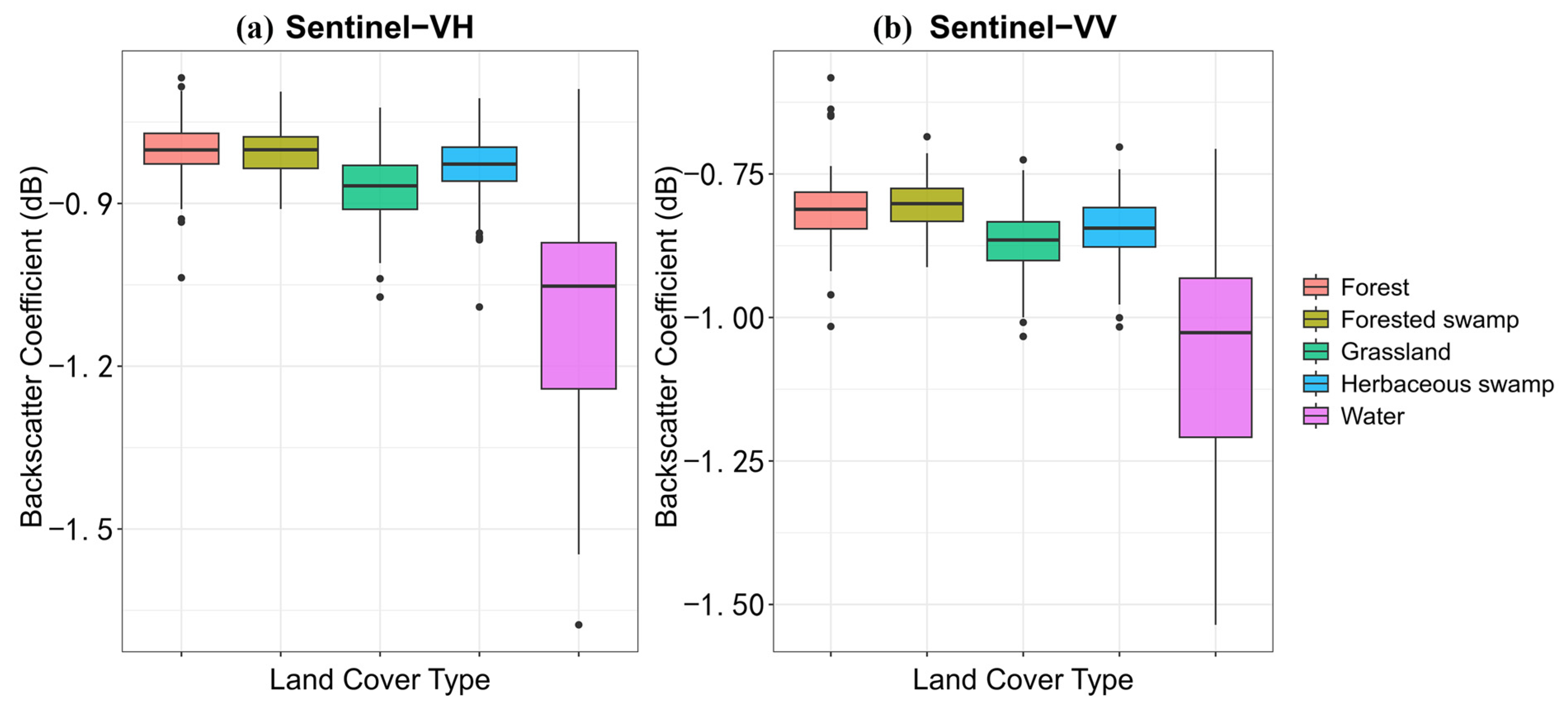
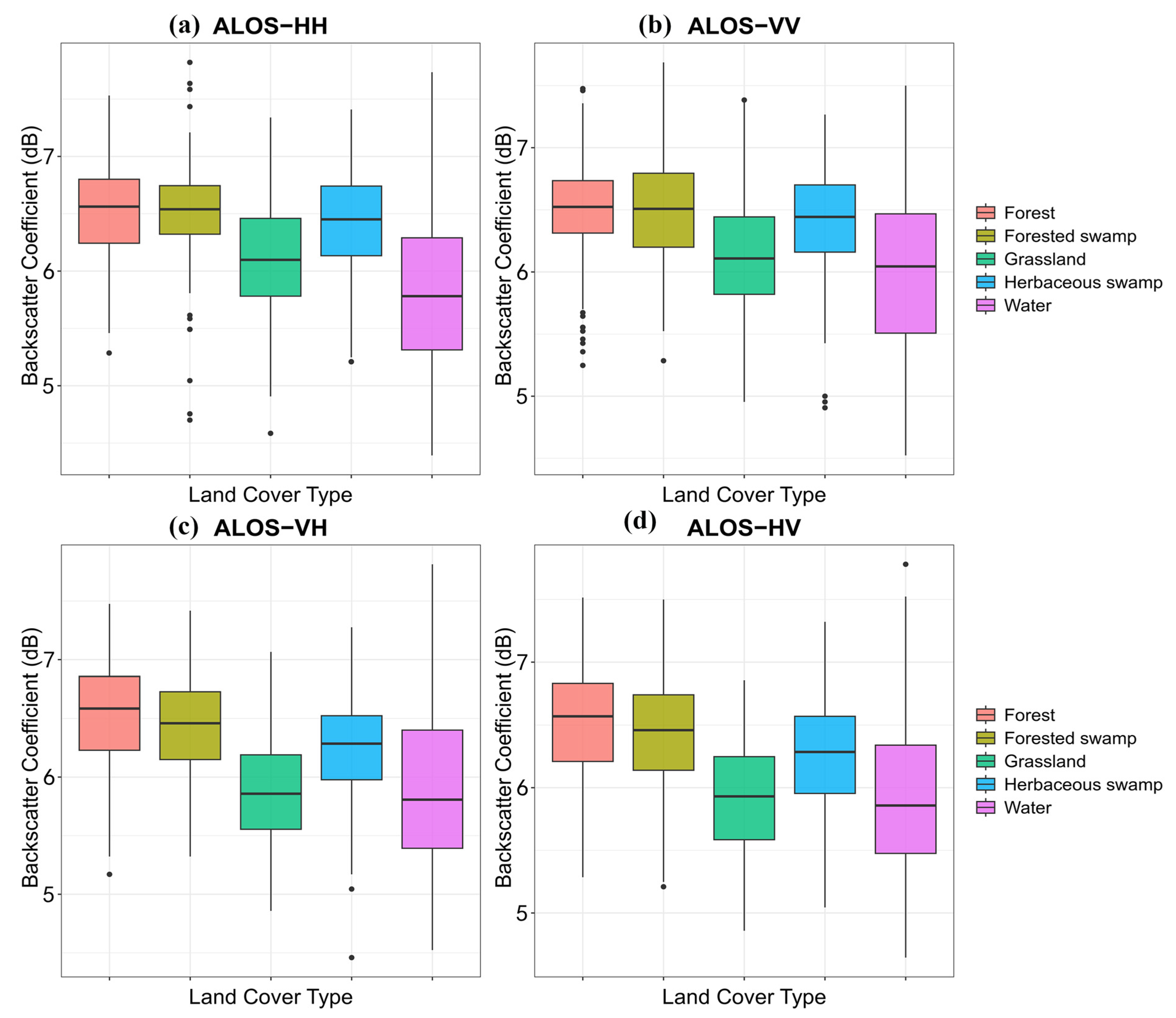
3.2. Differences in Polarimetric Backscattering Coefficients of Typical Land Cover Types
3.3. Hybrid Feature Weighting Fusion Strategy
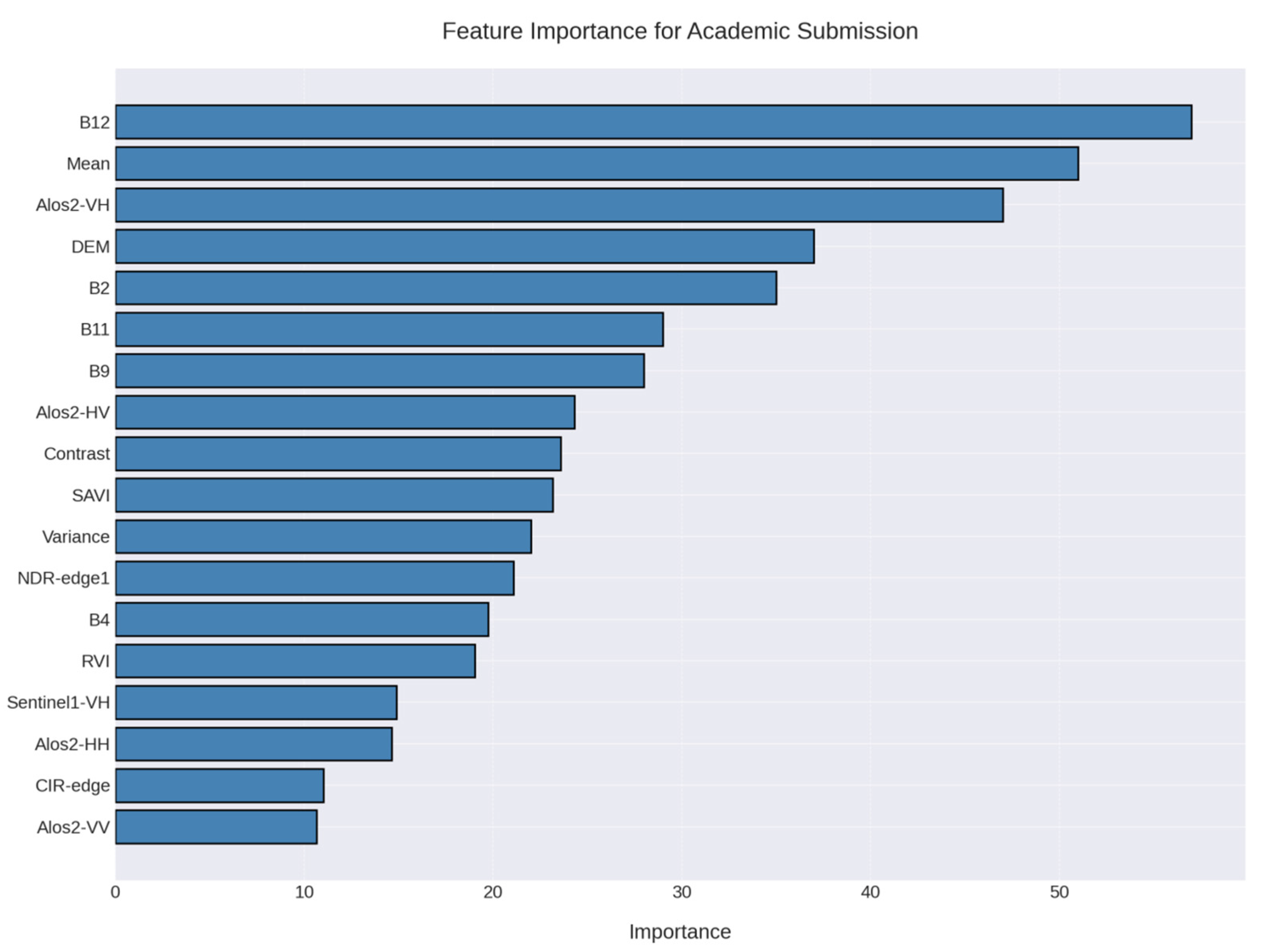
3.3.1. Feature Importance Assessment
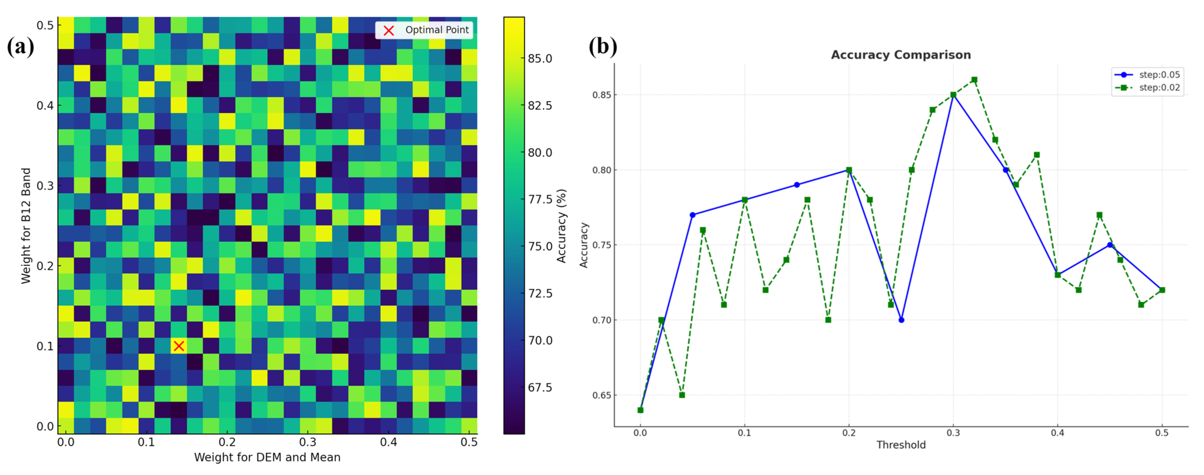
3.3.2. Stratified Weight Optimization
3.3.3. Multi-Source Feature Fusion
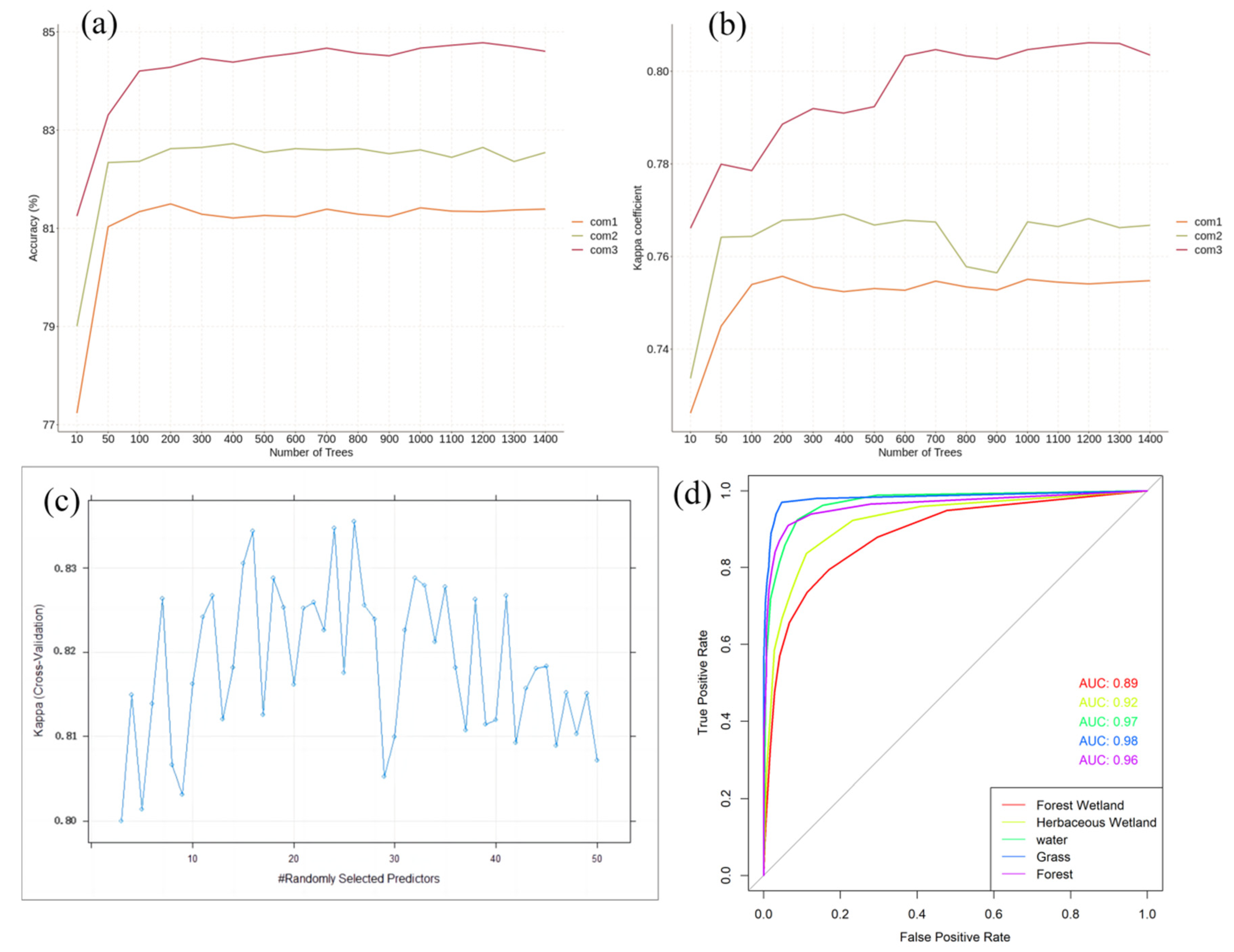
3.4. Modelling Results and Evaluation
4. Discussions
4.1. Methodological Innovations and Comparative Advantages
4.2. Key Findings and Ecological Implications
4.3. Limitations and Future Directions
5. Conclusions
Author Contributions
Funding
Data Availability Statement
Conflicts of Interest
Correction Statement
References
- Wang, B.W.; Mu, C.C.; Wang, B. Carbon storage of a primary coniferous forested wetland ecosystem in the temperate Changbai Mountain of China. Acta Ecol. Sin. 2019, 39, 3344–3354. [Google Scholar] [CrossRef]
- Zhang, S. Optimal planning algorithm of forest wetland tourism path based on GIS. Discret. Math. Sci. Cryptogr. 2018, 21, 393–397. [Google Scholar] [CrossRef]
- Rask, H.; Schoenau, J.; Anderson, D. Factors influencing methane flux from a boreal forest wetland in Saskatchewan, Canada. Soil Biol. Biochem. 2002, 34, 435–443. [Google Scholar] [CrossRef]
- Yang, Y.; Bian, H.; Yang, X. A review of forest wetland ecosystem service function and valuation. Wetl. Sci. Manag. 2017, 13, 61–64. [Google Scholar] [CrossRef]
- Zhu, D.; Ni, H.; Cui, F. Progress in the Restoration of Degraded Forest Wetland Ecosystems in the Daxing’anling Forest Area. Ter. Nat. Resour. 2013, 35, 61–63. [Google Scholar] [CrossRef]
- Song, F.; Su, F.L.; Mi, C.X.; Sun, D. Analysis of Driving Forces on Wetland Ecosystem Services Value Change: A Case in Northeast China. Sci. Total Environ. 2021, 751, 141778. [Google Scholar] [CrossRef]
- Tiner, R.W., Jr. Use of high-altitude aerial photography for inventorying forested wetlands in the United States. For. Ecol. Manag. 1990, 33, 593–604. [Google Scholar] [CrossRef]
- Brinson, M.M. A Hydrogeomorphic Classification for Wetlands; U.S. Army Engineer Waterways Experiment Station: Vicksburg, MS, USA, 1993. [Google Scholar]
- Hogg, A.R.; Todd, K.W. Automated Discrimination of Upland and Wetland Using Terrain Derivatives. Can. J. Remote Sens. 2007, 33 (Suppl. S1), S68–S83. [Google Scholar] [CrossRef]
- Yan, T.T.; Bian, H.F.; Liao, G.X.; Sheng, L.; Zhang, J.; Gao, M. Research Status of Remote Sensing Information Extraction Methods for Forest Wetlands. Remote Sens. Land Resour. 2014, 26, 11–18. [Google Scholar] [CrossRef]
- Lunetta, R.S.; Balogh, M.E. Application of Multi-Temporal Landsat 5 TM Imagery for Wetland Identification. Photogramm. Eng. Remote Sens. 1999, 65, 1303–1310. [Google Scholar]
- Sader, S.A.; Ahl, D.; Liou, W.S. Accuracy of Landsat-TM and GIS Rule-Based Methods for Forest Wetland Classification in Maine. Remote Sens. Environ. 1995, 53, 133–144. [Google Scholar] [CrossRef]
- Lin, Y.C.; Sarabandi, K. A Monte Carlo Coherent Scattering Model for Forest Canopies Using Fractal-Generated Trees. IEEE Trans. Geosci. Remote Sens. 1999, 37, 440–451. [Google Scholar] [CrossRef]
- Kwoun, O.; Lu, Z. Multi-Temporal RADARSAT-1 and ERS Backscattering Signatures of Coastal Wetlands in Southeastern Louisiana. Photogramm. Eng. Remote Sens. 2009, 75, 607–617. [Google Scholar] [CrossRef]
- Wang, J.F.; Mao, D.H.; Du, H.S.; Wang, Z.M. Mapping Swamps in Hani Wetland by Combining Sentinel-1/2 Satellite Images. Wetl. Sci. Manag. 2021, 17, 2–7. [Google Scholar]
- Lang, M.W.; Kasischke, E.S.; Prince, S.D.; Pittman, K.W. Assessment of C-Band Synthetic Aperture Radar Data for Mapping and Monitoring Coastal Plain Forested Wetlands in the Mid-Atlantic Region, USA. Remote Sens. Environ. 2008, 112, 4120–4130. [Google Scholar] [CrossRef]
- Cohen, J.; Lemmetyinen, J.; Ruiz, J.J. Detection of soil and canopy freeze/thaw state in the boreal region with L and C Band Synthetic Aperture Radar. Remote Sens. Environ. 2024, 305, 114102. [Google Scholar] [CrossRef]
- Lemmetyinen, J.; Ruiz, J.J.; Cohen, J. Attenuation of radar signal by a boreal forest canopy in winter. IEEE Geosci. Remote Sens. Lett. 2022, 19, 1–5. [Google Scholar] [CrossRef]
- Whitcomb, J.; Moghaddam, M.; McDonald, K.; Podest, E.; Kellndorfer, J. Wetlands Map of Alaska Using L-Band Radar Satellite Imagery. In Proceedings of the IEEE International Geoscience and Remote Sensing Symposium, Barcelona, Spain, 23–28 July 2007; pp. 2487–2490. [Google Scholar] [CrossRef]
- Corcoran, J.; Knight, J.; Brisco, B.; Kaya, S.; Cull, A.; Murnaghan, K. The Integration of Optical, Topographic, and Radar Data for Wetland Mapping in Northern Minnesota. Can. J. Remote Sens. 2011, 37, 564–582. [Google Scholar] [CrossRef]
- Xulu, S.; Mbatha, N.; Peerbhay, K.; Gebreslasie, M. Detecting Harvest Events in Plantation Forest Using Sentinel-1 and -2 Data via Google Earth Engine. Forests 2020, 11, 1283. [Google Scholar] [CrossRef]
- Dong, D.; Wang, C.; Yan, J.; He, Q. Combining Sentinel-1 and Sentinel-2 Image Time Series for Invasive Spartina alterniflora Mapping on Google Earth Engine: A Case Study in Zhangjiang Estuary. J. Appl. Remote Sens. 2020, 14, 044504. [Google Scholar]
- Samadzadegan, F.; Toosi, A.; Dadrass Javan, F. A Critical Review on Multi-Sensor and Multi-Platform Remote Sensing Data Fusion Approaches: Current Status and Prospects. Int. J. Remote Sens. 2025, 46, 1327–1402. [Google Scholar] [CrossRef]
- Li, J.; Zhang, J.; Yang, C.; Liu, H.; Zhao, Y.; Ye, Y. Comparative Analysis of Pixel-Level Fusion Algorithms and a New High-Resolution Dataset for SAR and Optical Image Fusion. Remote Sens. 2023, 15, 5514. [Google Scholar] [CrossRef]
- Pal, M. Random Forest Classifier for Remote Sensing Classification. Int. J. Remote Sens. 2005, 26, 217–222. [Google Scholar] [CrossRef]
- Mutanga, O.; Adam, E.; Cho, M.A. High Density Biomass Estimation for Wetland Vegetation Using WorldView-2 Imagery and Random Forest Regression Algorithm. Int. J. Appl. Earth Obs. Geoinf. 2012, 18, 399–406. [Google Scholar] [CrossRef]
- Whiteside, T.G.; Bartolo, R.E. Mapping Aquatic Vegetation in a Tropical Wetland Using High Spatial Resolution Multispectral Satellite Imagery. Remote Sens. 2015, 7, 11664–11694. [Google Scholar] [CrossRef]
- Bansal, M.; Goyal, A.; Choudhary, A. A Comparative Analysis of K-Nearest Neighbor, Genetic, Support Vector Machine, Decision Tree, and Long Short-Term Memory Algorithms in Machine Learning. Decis. Anal. J. 2022, 3, 100071. [Google Scholar] [CrossRef]
- Sheykhmousa, M.; Mahdianpari, M.; Ghanbari, H.; Mohammadimanesh, F.; Ghamisi, P.; Homayouni, S. Support Vector Machine Versus Random Forest for Remote Sensing Image Classification: A Meta-Analysis and Systematic Review. IEEE J. Sel. Top. Appl. Earth Obs. Remote Sens. 2020, 13, 6308–6325. [Google Scholar] [CrossRef]
- Zhang, Y.; Bergeron, Y.; Gao, L.; Zhao, X.; Wang, X.; Drobyshev, I. Tree Growth and Regeneration Dynamics at a Mountain Ecotone on Changbai Mountain, Northeastern China: Which Factors Control Species Distributions? Ecoscience 2014, 21, 387–404. [Google Scholar] [CrossRef]
- Yu, D.D.; Han, S.J. Ecosystem Service Status and Changes of Degraded Natural Reserves: A Study from the Changbai Mountain Natural Reserve, China. Ecosyst. Serv. 2016, 20, 56–65. [Google Scholar] [CrossRef]
- Hou, M.Z.; Li, L.; Yu, H.; Jin, R.; Zhu, W. Ecological Security Evaluation of Wetlands in Changbai Mountain Area Based on DPSIRM Model. Ecol. Indic. 2024, 160, 111773. [Google Scholar] [CrossRef]
- Lu, S.B.; Chen, Y.H.; Xu, W.L.; Zhu, W. Wetland Classification in the Changbai Mountain Nature Reserve. J. Beijing Norm. Univ. Nat. Sci. 2012, 28, 57–61. [Google Scholar]
- Plank, S.; Jüssi, M.; Martinis, S.; Twele, A. Mapping of Flooded Vegetation by Means of Polarimetric Sentinel-1 and ALOS-2/PALSAR-2 Imagery. Int. J. Remote Sens. 2017, 38, 3831–3850. [Google Scholar] [CrossRef]
- Sienaert, S. Usability of Sentinel-1 C-band VV and VH SAR Data for the Detection of Flooded Oil Palm. Master’s Thesis, Lund University, Lund, Sweden, 2023. [Google Scholar]
- Schwerdt, M.; Schmidt, K.; Ramon, N.T.; Alfonzo, G.C.; Doring, B.J.; Zink, M.; Prats-Iraola, P. Independent Verification of the Sentinel-1A System Calibration. IEEE J. Sel. Top. Appl. Earth Obs. Remote Sens. 2015, 9, 994–1007. [Google Scholar] [CrossRef]
- Gierszewska, M.; Berezowski, T. On the Role of Polarimetric Decomposition and Speckle Filtering Methods for C-Band SAR Wetland Classification Purposes. IEEE J. Sel. Top. Appl. Earth Obs. Remote Sens. 2022, 15, 2845–2860. [Google Scholar] [CrossRef]
- Liu, H.; Ren, H.; Niu, X.; Xia, P. Extraction of Cyanobacteria Bloom in Chaohu Lake Based on Sentinel-2 Remote Sensing Images. Ecol. Environ. 2021, 30, 146–150. [Google Scholar]
- Truckenbrodt, J.; Freemantle, T.; Williams, C.; Jones, T.; Small, D.; Dubois, C.; Thiel, C.; Rossi, C.; Syriou, A.; Giuliani, G. Towards Sentinel-1 SAR Analysis-Ready Data: A Best Practices Assessment on Preparing Backscatter Data for the Cube. Data 2019, 4, 93. [Google Scholar] [CrossRef]
- Du, C.; Ren, H.; Qin, Q.; Meng, J.; Zhao, S. A Practical Split-Window Algorithm for Estimating Land Surface Temperature from Landsat 8 Data. Remote Sens. 2015, 7, 647–665. [Google Scholar] [CrossRef]
- Liu, Y.; Zhu, Q.; Liao, K.; Lai, X.; Wang, J. Downscaling of ESA CCI Soil Moisture in Taihu Lake Basin: Are Wetness Conditions and Non-Linearity Important? J. Water Clim. Chang. 2021, 12, 1564–1579. [Google Scholar] [CrossRef]
- Wang, M.; Mao, D.; Wang, Y.; Xiao, X.; Xiang, H.; Feng, K.; Luo, L.; Jia, M.; Song, K.; Wang, Z. Wetland Mapping in East Asia by Two-Stage Object-Based Random Forest and Hierarchical Decision Tree Algorithms on Sentinel-1/2 Images. Remote Sens. Environ. 2023, 297, 113793. [Google Scholar] [CrossRef]
- Kreft, I.G.G.; De Leeuw, J.; Aiken, L.S. The Effect of Different Forms of Centring in Hierarchical Linear Models. Multivar. Behav. Res. 1995, 30, 1–21. [Google Scholar] [CrossRef]
- Feng, J.J.; Zhang, H.G.; Hu, X.J. The Scale Dependence of the Local Moran’s I. Stat. Appl. 2015, 4, 162–168. [Google Scholar] [CrossRef]
- Serneels, S.; De Nolf, E.; Van, E.P.J. Spatial Sign Pre-Processing: A Simple Way to Impart Moderate Robustness to Multivariate Estimators. J. Chem. Inf. Model. 2006, 46, 1402–1409. [Google Scholar] [CrossRef] [PubMed]
- Mallick, J.; Talukdar, S.; Shahfahad; Pal, S.; Rahman, A. A Novel Classifier for Improving Wetland Mapping by Integrating Image Fusion Techniques and Ensemble Machine Learning Classifiers. Ecol. Inform. 2021, 65, 101426. [Google Scholar] [CrossRef]
- Wu, F.; Ren, Y.; Wang, X. Application of Multi-Source Data for Mapping Plantation Based on Random Forest Algorithm in North China. Remote Sens. 2022, 14, 4946. [Google Scholar] [CrossRef]
- Budiman, F. SVM-RBF Parameters Testing Optimization Using Cross Validation and Grid Search to Improve Multiclass Classification. Sci. Vis. 2019, 11, 80–90. [Google Scholar] [CrossRef]
- Majnik, M.; Bosnić, Z. ROC Analysis of Classifiers in Machine Learning: A Survey. Intell. Data Anal. 2013, 17, 531–558. [Google Scholar] [CrossRef]
- Fawcett, T. An Introduction to ROC Analysis. Pattern Recognit. Lett. 2006, 27, 861–874. [Google Scholar] [CrossRef]
- Wang, Z. A New Clustering Method Based on Morphological Operations. Expert Syst. Appl. 2020, 145, 113102. [Google Scholar] [CrossRef]
- Yang, Y.G.; Wang, X.J.; Zhang, L.D.; Jian, L.; Tao, S.; Yao, J.; Guan, L.; Gao, S.; Wang, T.; Xiong, X. A Method for Wetland Information Extraction and Ecological Sensitivity Evaluation Based on Microwave Remote Sensing and Optical Remote Sensing Technologies. CN Patent 107862255A, 23 April 2025. [Google Scholar]
- Touzi, R.; Shimada, M.; Motohka, T. Calibration and Validation of Polarimetric ALOS-2 PALSAR-2. Remote Sens. 2022, 14, 2452. [Google Scholar] [CrossRef]
- Liang, J.; Pan, J. Identifying Carbon Sequestration’s Priority Supply Areas from the Standpoint of Ecosystem Service Flow: A Case Study for Northwestern China’s Shiyang River Basin. Sci. Total Environ. 2024, 927, 172283. [Google Scholar] [CrossRef]
- Bradley, A.P. The Use of the Area Under the ROC Curve in the Evaluation of Machine Learning Algorithms. Pattern Recognit. Lett. 1997, 30, 1145–1159. [Google Scholar] [CrossRef]
- Xiang, H.; Yu, F.; Bai, J.; Shi, X.; Wang, M.; Yan, H.; Xi, Y.; Wang, Z.; Mao, D. SHAP-DNN Approach Advances Remote Sensing Mapping of Forested Wetlands. IEEE J. Sel. Top. Appl. Earth Obs. Remote Sens. 2025, 18, 6859–6869. [Google Scholar] [CrossRef]
- Ali, A.M.; Darvishzadeh, R.; Shahi, K.R.; Skidmore, A. Validating the Predictive Power of Statistical Models in Retrieving Leaf Dry Matter Content of a Coastal Wetland from a Sentinel-2 Image. Remote Sens. 2019, 11, 1936. [Google Scholar] [CrossRef]


| Class I | Class II | Precise Definition |
|---|---|---|
| Natural wetland | Water | Permanent or seasonal freshwater bodies (rivers, lakes) with stable hydrological regimes. |
| Forest swamp | Freshwater wetlands dominated by woody vegetation (tree cover >30%, height >5 m). | |
| Herbaceous swamp | Wetlands dominated by emergent hydrophytic herbs (e.g., Carex spp., height <2 m). | |
| Human-made wetland | Paddy field | Flooded fields bounded by embankments for rice cultivation, with seasonal inundation. |
| Dryland | Dryland without irrigation facilities primarily relying on natural precipitation for cultivating drought-tolerant crops | |
| Non-wetland | Forest | Upland areas with continuous tree cover (natural or planted), lacking wetland hydrology. |
| Grassland | Lands dominated by herbaceous or shrub vegetation, used for grazing or natural meadows. | |
| Impervious | Artificial surfaces (e.g., buildings, roads) with minimal vegetation or soil exposure. |
| Feature Category | Feature Sub-Category | Feature Name (Number) | Data Source |
|---|---|---|---|
| Polarization | Polarization bands | VV, VH (2) | Sentinel-1 |
| VV, VH, HV, HH (4) | ALOS-2/PALSAR | ||
| Polarization indices | VV + VH, VH-VV, VH/VV (3) | Sentinel-1 | |
| Spectral | Spectral bands | B1~B12 (13) | |
| Vegetation indices | Normalized Difference Vegetation Index (NDVI), Difference Vegetation Index (DVI), Ratio Vegetation Index (RVI), Soil-Adjusted Vegetation Index (SAVI) (4) | Sentinel-2 | |
| Red edge indices | (Normalized Difference Vegetation Index Red-edge) NDVIR-edge1, NDVIR-edge2, NDVIR-edge3, Normalized Difference Red-edge (NDR-edge1), NDR-edge2, Chlorophyll Index Red-edge (CIR-edge) (6) | ||
| Water indices | Normalized Difference Water Index (NDWI), Modified Normalized Difference Water Index (MNDWI), Normalized Difference Snow Index (NDSI), hermal Sensitivity Index (SI-T) (4) | ||
| Texture | Mean, Variance, Maximum Probability, Entropy, Homogeneity, Correlation, Dissimilarity, Contrast, Angular Second Moment (9) | ||
| Terrain | Brightness, Wetness (2) | DEM | |
| Land surface temperature (LST) | Surface temperature estimate | LST (1) | Landsat-8 |
| Type | Forested Swamp | Herbaceous Swamp | Water | Grassland | Forest |
|---|---|---|---|---|---|
| Training Samples | 392 | 312 | 218 | 144 | 409 |
| Test Samples | 168 | 134 | 94 | 62 | 175 |
| Sum | 560 | 446 | 312 | 205 | 584 |
| Ture | ||||||||
|---|---|---|---|---|---|---|---|---|
| Samples Number | Forested Swamp | Herbaceous Swamp | Water | Grassland | Forest | Summary | User’s Accuracy | |
| Imitate | Forested swamp | 172 | 12 | 6 | 0 | 8 | 198 | 86.87% |
| Herbaceous swamp | 30 | 223 | 5 | 4 | 3 | 265 | 84.15% | |
| Water | 1 | 4 | 108 | 2 | 0 | 115 | 93.91% | |
| Grassland | 1 | 3 | 2 | 58 | 2 | 66 | 87.88% | |
| Forest | 8 | 0 | 2 | 0 | 194 | 204 | 95.10% | |
| Summary | 212 | 242 | 123 | 64 | 207 | 848 | ||
| Producer’s accuracy | 80.37% | 90.28% | 81.20% | 90.63% | 93.27% | |||
| Overall accuracy | 87.18% | Kappa | 0.8343 | |||||
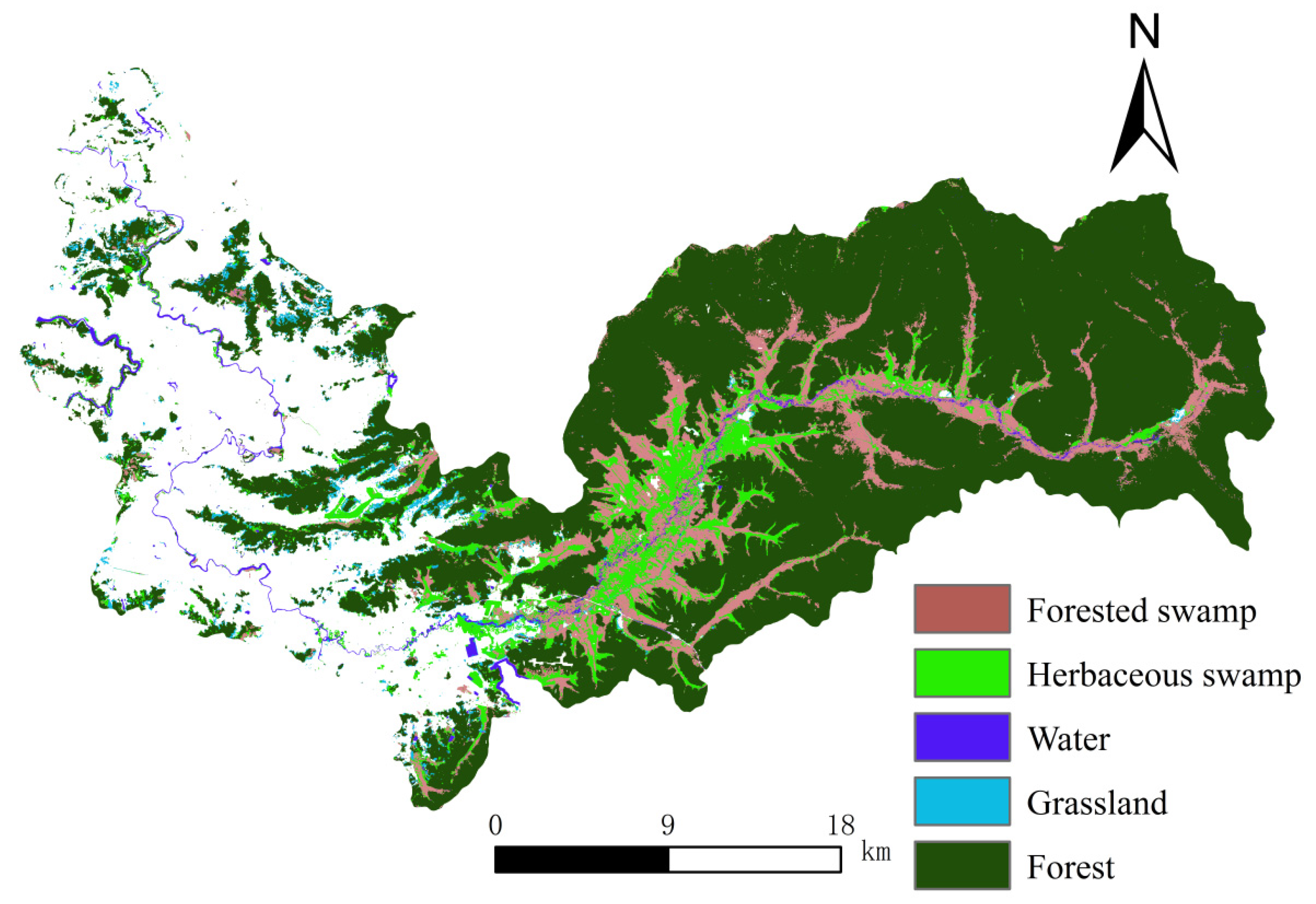
| Type | Forested Swamp | Herbaceous Swamp | Water | Grassland | Forest | Impervious |
|---|---|---|---|---|---|---|
| Area/km2 | 125.89 | 86.61 | 17.45 | 22.3 | 743.28 | 18.95 |
| Percentage | 9.00% | 6.19% | 1.25% | 1.59% | 53.13% | 1.35% |
Disclaimer/Publisher’s Note: The statements, opinions and data contained in all publications are solely those of the individual author(s) and contributor(s) and not of MDPI and/or the editor(s). MDPI and/or the editor(s) disclaim responsibility for any injury to people or property resulting from any ideas, methods, instructions or products referred to in the content. |
© 2025 by the authors. Licensee MDPI, Basel, Switzerland. This article is an open access article distributed under the terms and conditions of the Creative Commons Attribution (CC BY) license (https://creativecommons.org/licenses/by/4.0/).
Share and Cite
Lv, J.; Liu, Y.; Jin, R.; Zhu, W. Forested Swamp Classification Based on Multi-Source Remote Sensing Data: A Case Study of Changbai Mountain Ecological Function Protection Area. Forests 2025, 16, 794. https://doi.org/10.3390/f16050794
Lv J, Liu Y, Jin R, Zhu W. Forested Swamp Classification Based on Multi-Source Remote Sensing Data: A Case Study of Changbai Mountain Ecological Function Protection Area. Forests. 2025; 16(5):794. https://doi.org/10.3390/f16050794
Chicago/Turabian StyleLv, Jing, Yuyan Liu, Ri Jin, and Weihong Zhu. 2025. "Forested Swamp Classification Based on Multi-Source Remote Sensing Data: A Case Study of Changbai Mountain Ecological Function Protection Area" Forests 16, no. 5: 794. https://doi.org/10.3390/f16050794
APA StyleLv, J., Liu, Y., Jin, R., & Zhu, W. (2025). Forested Swamp Classification Based on Multi-Source Remote Sensing Data: A Case Study of Changbai Mountain Ecological Function Protection Area. Forests, 16(5), 794. https://doi.org/10.3390/f16050794