Research on Protective Forest Change Detection in Aral City Based on Deep Learning

Abstract

Protective forests play a crucial role in ecosystems, particularly in arid and semi-arid regions, where they provide irreplaceable ecological functions such as windbreaks, sand fixation, soil and water conservation, and climate regulation. This study selects Aral City in Xinjiang as the research area and proposes a method that integrates high-resolution remote sensing data (GF-2) with a Spatiotemporal Attention Neural Network (STANet) model to improve the accuracy of protective forest change detection. The study utilizes GF-2 remote sensing imagery and employs a spatiotemporal attention mechanism to incorporate spatial and temporal information, overcoming the limitations of traditional methods in processing long-term time-series remote sensing data. The results demonstrate that the combination of GF-2 imagery and the STANet model effectively detects protective forest changes in Aral City, achieving an F1-score of 83.64% and an accuracy of 78.52%, indicating significant detection capability. Spatial analysis based on the change detection results reveals notable changes in the protective forest area within the study region, with a decline in vegetation coverage in certain areas. This study suggests that the STANet method has strong application potential in protective forest change detection in arid regions, providing precise spatiotemporal change information for protective forest restoration and management. The findings offer a scientific basis for ecological restoration and sustainable development in Aral City, Xinjiang, and are of great significance for improving protective forest management and land use decision-making.

1. Introduction

Protective forests are a vital component in maintaining ecological balance, playing a key role in windbreaks, sand fixation, soil and water conservation, climate regulation, and biodiversity protection [1]. However, in recent years, global climate change and intensified human activities have posed severe challenges to the spatial distribution and ecological functions of protective forests. Many regions are experiencing forestland degradation, reduced vegetation cover, and declining ecosystem stability. This trend is particularly evident in arid and semi-arid regions, where factors such as agricultural expansion, urbanization, and water resource shortages have accelerated protective forest degradation [2]. Therefore, accurately monitoring the spatiotemporal dynamics of protective forests is essential for scientifically assessing their ecological benefits, optimizing land use management, and formulating ecological restoration policies.

Traditional protective forest investigations primarily rely on field surveys and statistical data analysis. While these methods provide high-accuracy local information, they are costly, time-consuming, and labor-intensive for large-scale and long-term monitoring. With the rapid advancement of remote sensing technology, remote sensing-based monitoring methods have emerged as the primary approach for vegetation monitoring and change detection due to their advantages in large-scale coverage, periodic observation, and objectivity [3]. Optical remote sensing data (e.g., Landsat, MODIS, and “GF-2”) can be used to extract vegetation indices and forest cover to analyze the dynamic changes in protective forests. Additionally, Synthetic Aperture Radar (SAR) data (e.g., Sentinel-1) have played a crucial role in protective forest monitoring due to their all-weather, all-time observation capability, which is unaffected by atmospheric conditions.

The long-term changes in forest cover mainly include transitions between forests and other land cover types, as well as transformations within different forest types [4]. These changes have significant impacts on the global ecological environment, climate change, and biodiversity. Traditional forest resource surveys primarily rely on ground measurements, which suffer from inefficiencies, long cycles, poor timeliness, and high susceptibility to human errors, making it difficult to meet the current demands for forest resource change monitoring. In recent years, with the advancement of aerospace remote sensing technology, remote sensing has demonstrated significant advantages in resource change detection due to its high data acquisition efficiency, wide detection range, and periodic observation capabilities, and it has been widely applied in monitoring dynamic changes in forest resources. Currently, various remote sensing techniques are used for forest cover change detection, among which the direct analysis comparison method and the post-classification comparison method are widely applied in research. The direct analysis comparison method directly compares pixel information differences of the same region at different time phases to determine the location and extent of changes. In contrast, the post-classification comparison method first classifies images based on the same standard and then compares the classification results to identify changes. In the field of forest cover change detection, numerous studies have adopted different approaches to analyze changes in land cover types. Huang et al. [5] proposed an automatic change detection method for multi-temporal remote sensing images based on a two-dimensional Otsu algorithm improved by the Firefly algorithm. This method effectively and rapidly extracts change areas between multi-temporal remote sensing images. Li et al. [6] utilized multi-temporal Landsat TM images combined with machine learning methods, such as Support Vector Machines (SVMs) and Random Forest (RF) classifiers, for forest classification and change analysis. Their study demonstrated that machine learning methods could significantly improve forest classification accuracy while also revealing the applicability of different algorithms in change detection. Reddy et al. [7] conducted a long-term forest cover change monitoring study (1920–2013) in the Western Ghats biodiversity hotspot in India. By using multi-source remote sensing data, they analyzed the spatiotemporal patterns of forest cover change and explored its driving factors. Wessels et al. [8] proposed a change detection method based on a Random Forest classifier to rapidly update land cover maps. Their study showed that this method effectively improved classification accuracy for land cover categories and enhanced the robustness of change detection. Additionally, research has shown progress in applying an SVM to forest cover change detection. For instance, some studies have employed an SVM for remote sensing image change detection, successfully monitoring the status and dynamic changes of land cover. Rocha [9] introduced an approach that integrates Topological Data Analysis (TDA) and artificial intelligence to enhance the ability to forecast social trends. Some aspects of this research may also have potential applications in remote sensing, particularly in the automatic extraction and classification of forest training samples. De Bem et al. [10] applied Convolutional Neural Networks (CNNs) and Landsat data for deforestation change detection in the Brazilian Amazon. Their study demonstrated that deep learning methods have strong potential for extracting change features from remote sensing images. Overall, machine learning methods have shown high accuracy and reliability in forest cover change detection. However, due to their complexity, they tend to be less practical, and their stability in detecting changes in complex terrain remains a challenge.

Currently, protective forest change detection is primarily based on multi-temporal or bi-temporal remote sensing data, with commonly used methods including vegetation index trend analysis [11], post-classification comparison [12], and Object-Based Image Analysis (OBIA) [13,14]. Pixel-based methods such as trend analysis and post-classification comparison are often prone to “salt-and-pepper noise” when dealing with complex backgrounds and high-noise data, which can reduce detection accuracy. While OBIA effectively mitigates such noise through object-level analysis, its overall accuracy may still be affected by segmentation errors and feature selection strategies. In recent years, deep learning techniques have been widely applied in remote sensing change detection due to their strong feature extraction capabilities and ability to learn automatically. Methods such as Convolutional Neural Networks (CNNs) [15], Fully Convolutional Networks (FCNs) [16], Recurrent Neural Networks (RNNs) [17], and attention mechanisms [18,19] (e.g., Transformer, Mamba) have been successfully employed in vegetation change detection, achieving significant improvements in accuracy. However, traditional deep learning methods primarily focus on spatial feature extraction and do not fully utilize the spatiotemporal information inherent in remote sensing data, particularly when detecting long-term changes.

To further enhance the accuracy and reliability of protective forest change detection, this study employs the Spatial-Temporal Attention Neural Network (STANet) [20] for protective forest change detection. STANet effectively integrates spatial and temporal information from remote sensing imagery, reducing noise interference and improving change detection accuracy. The study focuses on Aral City in Xinjiang, which is located on the northern edge of the Tarim Basin and represents a typical arid oasis ecosystem. Aral City has long relied on protective forest systems to mitigate wind erosion and improve agricultural production conditions. However, due to land use changes and water resource management adjustments, some protective forests in the region have shown signs of degradation, necessitating refined change detection techniques to assess their spatiotemporal evolution. By integrating high-resolution GF-2 remote sensing data with the STANet model, this study aims to develop a protective forest change detection method suitable for arid regions, providing a scientific basis for ecological conservation and sustainable development in Aral City, Xinjiang.

The main objectives of this study are as follows:

(1)

Explore the potential of GF-2 remote sensing data in protective forest change monitoring, with a focus on its ability to capture subtle variations in high-resolution imagery. This task aims to leverage the high spatial resolution of GF-2 data to enhance the detection of fine-scale changes in forest cover, which is critical for understanding the dynamics of protective forests in arid regions.

(2)

Evaluate the effectiveness of the STANet-based deep learning approach in detecting protective forest changes under complex environmental conditions.

(3)

Analyze the spatial characteristics of protective forest in Aral City, providing decision-making support for regional ecological restoration and forestland management.

2. Research Area and Method

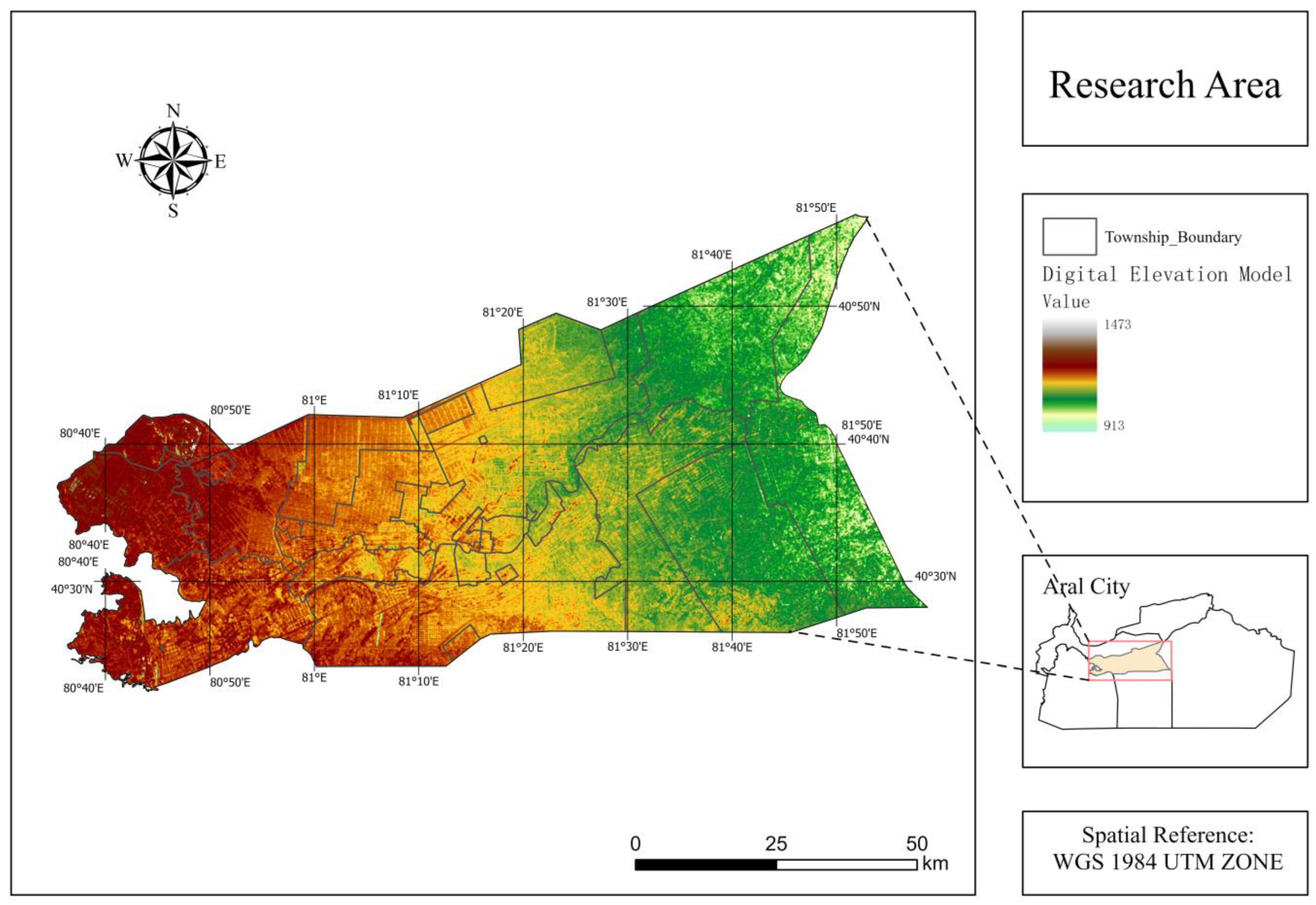
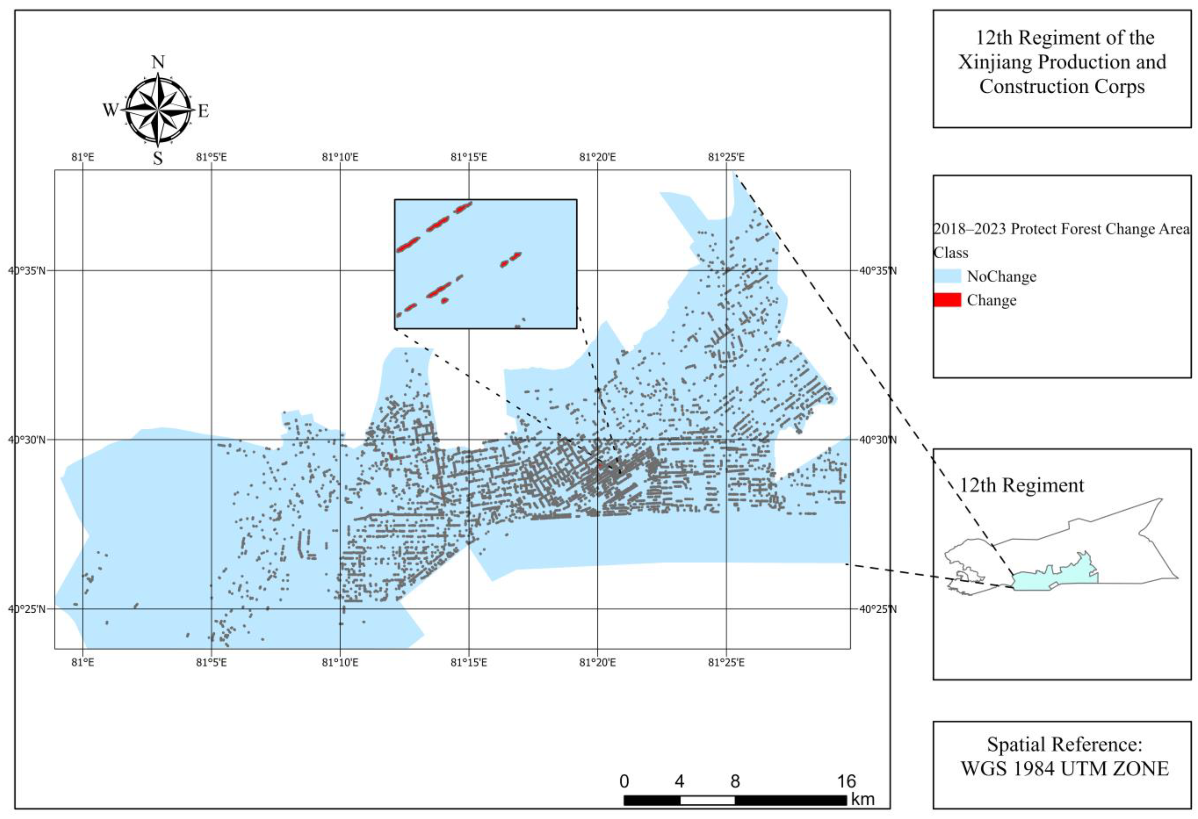
2.1. Research Area

Aral City is located in the southern part of Xinjiang Uygur Autonomous Region, China, at the intersection of the southern foothills of the Tianshan Mountains and the northern edge of the Tarim Basin. Its geographical coordinates are approximately 40°30′56″ N and 81°15′49″ E. Aral City is administered by the First Division of the Xinjiang Production and Construction Corps (XPCC) and covers a total administrative area of approximately 3927.10 square kilometers. The city is bordered by Aksu City to the east, Hotan Prefecture to the south, Kashgar Prefecture to the west, and Tacheng Prefecture to the north, as shown in Figure 1.

Aral City has a warm temperate, extremely continental arid desert climate, characterized by significant seasonal variations and arid conditions. The average annual temperature is approximately 12.4 °C, with relatively high temperatures and substantial diurnal temperature differences. The extreme annual temperature range is wide, with a maximum recorded temperature of 40.6 °C and a minimum of −17.3 °C. The average annual precipitation is only about 56.8 mm, primarily concentrated in the summer months, making it a typical arid region. The city receives abundant sunshine, with an annual sunshine percentage of approximately 58%, which, despite a slight decline in recent years, remains higher than in many other arid regions. Due to its arid conditions and high wind speeds, Aral City frequently experiences sandstorms, with maximum wind speeds reaching 12.4 m per second, predominantly from the west. These climatic conditions pose significant challenges for protective forest growth while also providing a unique research context for monitoring protective forest changes.

The ecological environment of Aral City exhibits typical arid and semi-arid characteristics, with relatively simple vegetation types yet relatively rich biodiversity. The primary plant species in the area include Populus euphratica (desert poplar), Populus pruinosa (gray poplar), Populus diversifolia (bitter poplar), Elaeagnus angustifolia (Russian olive), Tamarix ramosissima (red willow), and Salix psammophila (desert willow). These plants play a crucial role in wind and sand resistance, soil conservation, and environmental improvement. In addition, herbaceous plants such as Apocynum venetum (luobuma), Phragmites australis (common reed), Typha angustifolia (narrowleaf cattail), Agropyron cristatum (crested wheatgrass), and Lespedeza davurica (Daurian lespedeza) are distributed in specific regions. The vegetation of Aral City is closely linked to its ecosystem and plays a vital role in the construction and monitoring of protective forest.

In recent years, Aral City has made significant progress in ecological protection. In response to desertification issues, the city has implemented continuous ecological water replenishment projects to improve vegetation conditions on the desert margins. Meanwhile, afforestation, desertification control, and other ecological restoration measures have effectively enhanced regional environmental quality. The construction and protection of protective forest not only contribute to wind and sand mitigation but also play a crucial role in restoring regional ecological balance.

From the perspective of remote sensing and deep learning-based analysis, monitoring the dynamics of protective forest vegetation in Aral City presents both challenges and opportunities. High-resolution remote sensing data (e.g., GF-2) provide detailed spatial and temporal information for protective forest analysis, while deep learning models such as the Spatial-Temporal Attention Neural Network (STANet) enable the extraction of fine-grained change patterns under complex environmental conditions. By integrating multi-temporal remote sensing observations with deep learning-based change detection techniques, this study aims to provide a comprehensive assessment of protective forest dynamics in Aral City, contributing to regional ecological conservation and sustainable development.

2.2. Dataset

This study utilized “GF-2” satellite imagery as the data source, acquiring both panchromatic (0.8 m resolution) and multispectral (blue, green, red, near-infrared; 3.2 m resolution) data for the 2018 and 2023 acquisition periods. The Gram–Schmidt fusion algorithm implemented in the ENVI 5.6 platform was employed to merge the panchromatic and multispectral images, thereby generating enhanced multispectral imagery with a spatial resolution of 0.8 m. Based on the fused imagery, the red, green, and blue bands were extracted to synthesize true-color images, which served as the foundational dataset for subsequent analyses.

To eliminate geometric misalignments between the multi-temporal images, Ground Control Points (GCPs) were used to perform orthorectification on the datasets from both periods, and a second-order polynomial transformation model was applied to achieve sub-pixel level co-registration (with RMSE < 0.5 pixels), thus ensuring spatiotemporal comparability. Figure 2 illustrates the GF-2 satellite imagery for the 2018 T1 period (left), the 2023 T2 period (center), and the annotated label mask (right). By comparing the T1 and T2 images, the changes in protective forest conditions between 2018 and 2023 can be clearly observed; the label mask is used to delineate protective forest change areas (with white indicating change and black indicating no change). These labels were generated using the “Label Objects for Deep Learning” tool in ArcGIS Pro 3.0.2 and calibrated with field validation data to ensure accuracy.

Within the ArcGIS Pro 3.0.2 environment, based on visual interpretation and field validation data, the “Label Objects for Deep Learning” tool was employed to annotate the protective forest change areas in both datasets, thereby constructing pixel-level change labels. Subsequently, the “Export Training Data for Deep Learning” tool was used to segment the imagery into 256 × 256-pixel tiles, with a 20% overlap set to preserve edge change features. The tiles were saved in TIFF format, and binary label masks were generated simultaneously. The 20% overlap in the image tiles offers several advantages for capturing edge features. First, the overlap ensures that the same sample can appear in multiple tiles; if a sample near the edge in one tile undergoes significant attenuation, it may appear at the center of another tile with greater weight, thereby complementing the sample information and reducing edge effects. Second, the sharing of samples between tiles prevents the loss of frequency information at the boundaries that might occur without overlap, enhancing signal integrity and the comprehensiveness of feature extraction. Additionally, averaging features across overlapping tiles helps to reduce the influence of random noise, yielding smoother feature estimates that are closer to the true signal. Finally, overlapping reduces the dependency on any single tile for feature estimation, thus lowering noise sensitivity and improving the stability and reliability of the results. Collectively, these improvements ensure that edge features are captured and utilized more accurately in subsequent analyses, significantly enhancing overall detection accuracy and reliability. The constructed dataset includes both positive samples (protective forest change areas) and negative samples (unchanged areas), covering various types of protective forest changes. In total, the dataset comprises 2587 groups of sample images (triplets consisting of pre-event, post-event, and ground truth labels). The annotated samples were randomly divided into a training set (80%) and a validation set (20%) to ensure consistent spatial-temporal distribution between the two periods. It is important to note that the training and validation sets were derived from the same dataset, and given the use of tiled imagery, there may be some spatial overlap between samples. As such, the validation set cannot be considered fully independent, which may lead to optimistic accuracy estimates.

The GF-2 deep learning dataset for protective forest in arid regions fills a sub-meter change detection data gap and is capable of capturing micro-scale ecological degradation signals that traditional medium-resolution imagery cannot detect. The precisely annotated protective forest change patches in this dataset not only provide critical support for evaluating the effectiveness of the Tarim River Basin Ecological Protection and Restoration Plan but also offer a spatial decision-making basis for dust source management and ecological water quota optimization. 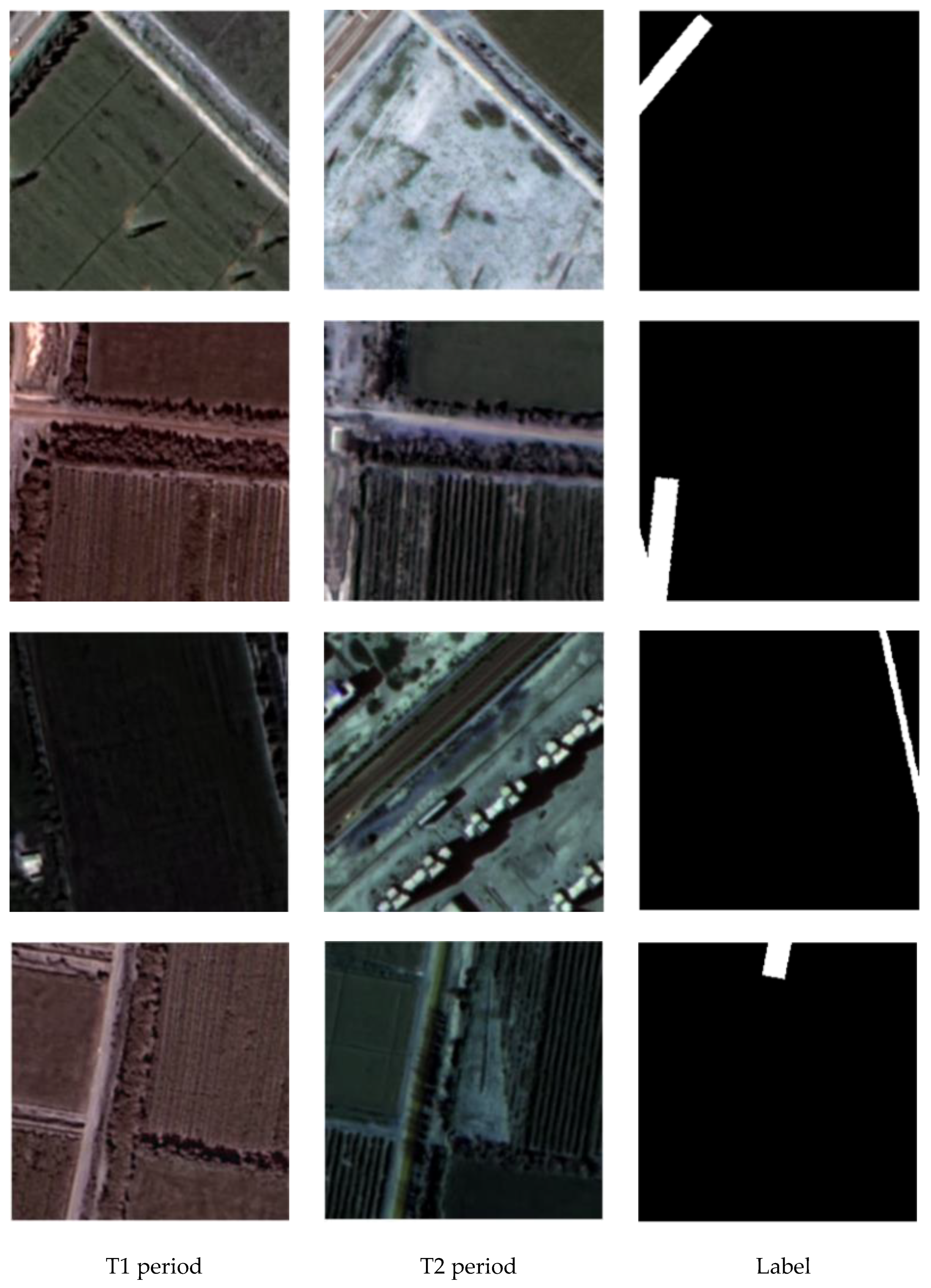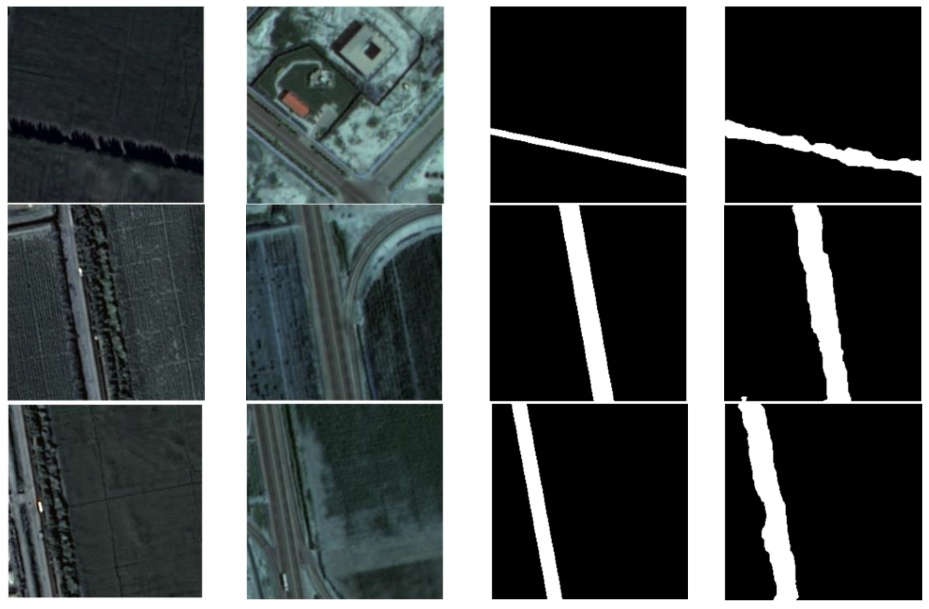Moreover, by quantifying the hotspots of protective forest degradation and expansion trends, this dataset contributes to the assessment of carbon sink potential in arid regions under the “dual carbon” objectives, thereby providing scientific support for regional ecological restoration and sustainable development.

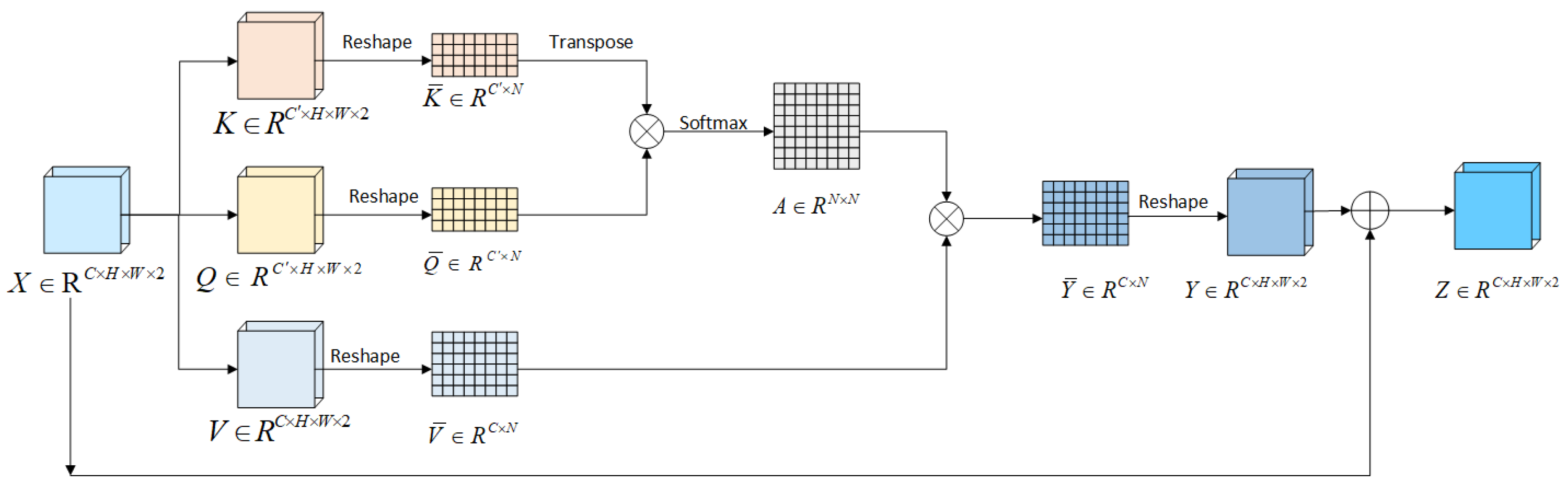
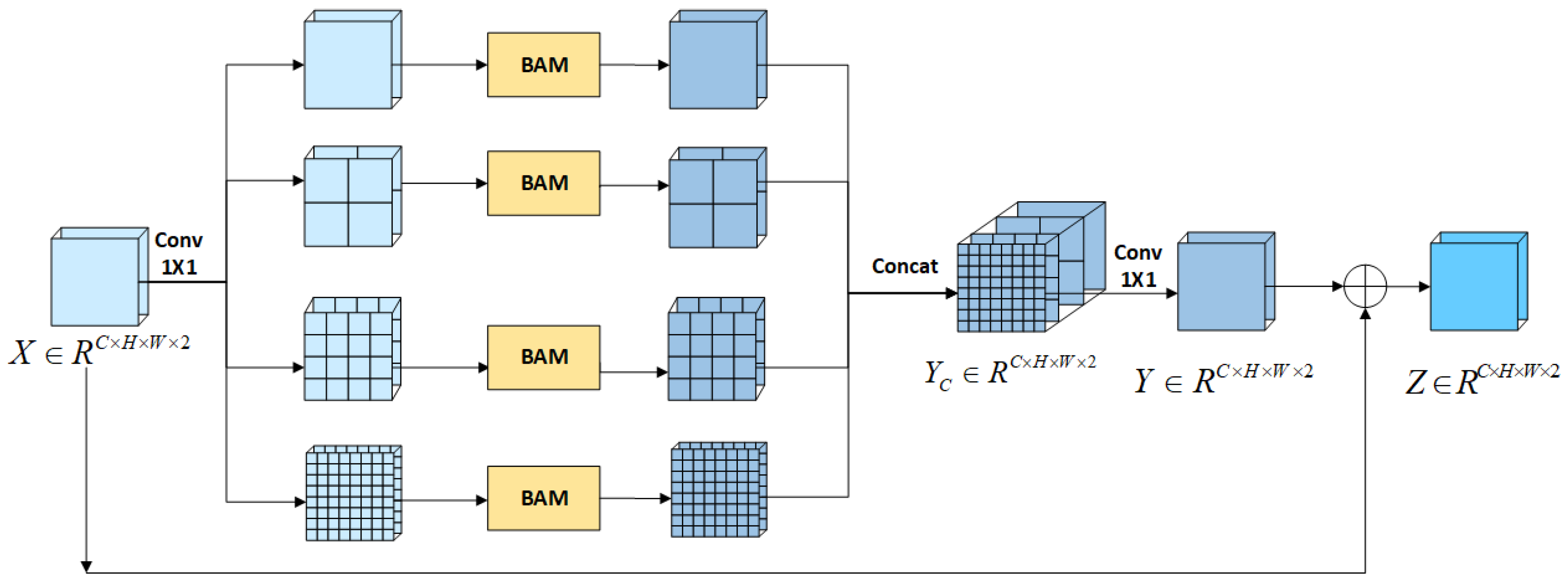
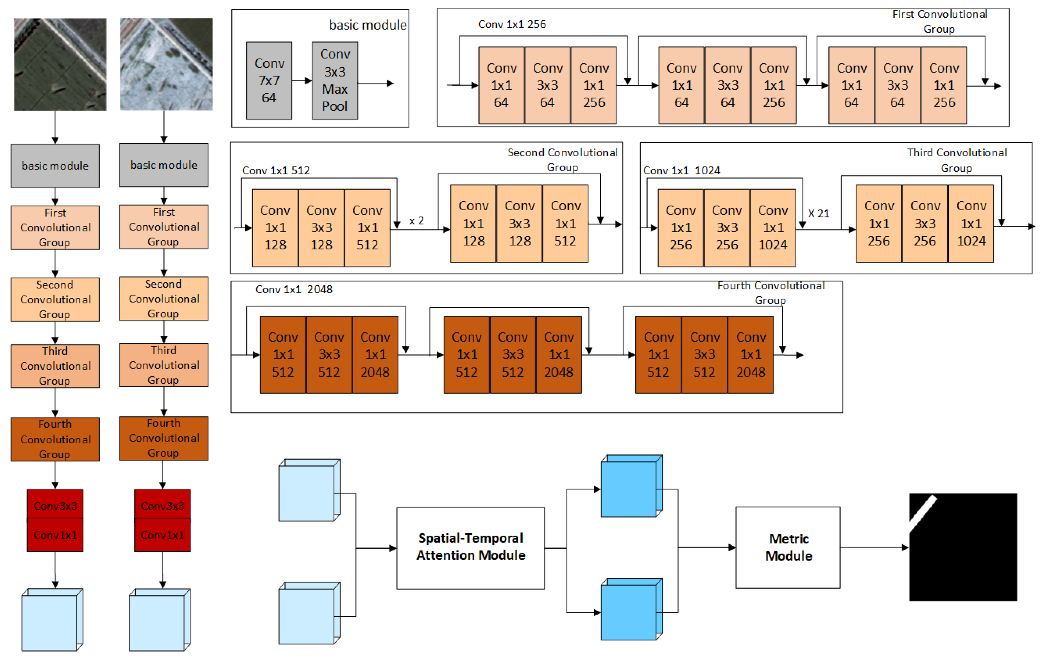
2.3. Deep Learning Model

With the continuous advancement of remote sensing technology, change detection has become a crucial task in environmental monitoring and land use research. Traditional change detection methods primarily rely on threshold-based and image differencing algorithms. While simple and efficient, these methods often struggle with low accuracy and robustness in complex environments. In recent years, deep learning, particularly Convolutional Neural Networks (CNNs), has made significant progress in image processing, enabling the automatic learning of multi-level feature representations from data. This makes CNNs particularly well-suited for large-scale and complex remote sensing image analysis. Deep learning, through end-to-end training, effectively circumvents the difficulties and limitations of manual feature selection by automatically extracting rich spatial and textural features from raw data. As a result, it has been widely applied to tasks such as remote sensing image classification, change detection, and object recognition. In particular, Residual Network (ResNet)-based methods [14] have demonstrated strong capabilities in image recognition due to their deep network architecture. U-Net has achieved remarkable success in medical image segmentation due to its symmetric encoder–decoder structure and skip connections [21]. However, its architecture requires modifications and optimizations to accommodate the characteristics of multi-temporal remote sensing images for change detection tasks. Peng, Zhang, and Guan [22] proposed an end-to-end change detection method for high-resolution satellite images based on the U-Net++ architecture. By employing nested and dense skip connections, their method enhances multi-scale feature fusion, leading to significant improvements in the mean Intersection over Union (mIoU) in very high-resolution change detection tasks. Additionally, Seo, Park, and Kim [23] introduced a feature-based change detection approach specifically designed for detecting small objects in high-resolution satellite images. Their method effectively extracts critical features in change regions, thereby improving detection accuracy. With the advancement of deep learning techniques, attention mechanisms have played an increasingly crucial role in remote sensing change detection. Zhang et al. [24] proposed the CD-Mamba model, which integrates the Mamba state space model (SSM) with local feature information to enhance change detection in remote sensing imagery. Their study demonstrates that this approach achieves superior performance in binary change detection tasks and improves the identification of subtle change regions.

Overall, deep learning methods based on U-Net and its improved architectures have shown high applicability in remote sensing change detection. Moreover, models incorporating Transformer or Mamba mechanisms further enhance the capture of critical change features, offering promising directions for future advancements in remote sensing change detection methodologies.

However, while U-Net performs well in semantic segmentation tasks, it primarily focuses on local spatial features and struggles to fully capture the dynamic changes embedded in time-series data. Transformer and Mamba models, despite their strong capability in capturing global long-range dependencies, suffer from high computational complexity and heavy dependence on large-scale training data, limiting their efficient deployment in high-resolution remote sensing change detection. Against this backdrop, the STANet model has emerged as a promising approach due to its unique spatiotemporal attention mechanism. STANet incorporates the Basic Attention Module (BAM) and the Pyramid Attention Module (PAM) within an encoder–decoder framework, enabling efficient integration of spatial and temporal information while effectively reducing noise interference. This facilitates accurate detection of complex spatiotemporal changes. Compared to U-Net and Transformer-based models, STANet offers several notable advantages: it fully exploits the dynamic information in multi-temporal remote sensing images, capturing not only local spatial features but also long-term change trends, which is particularly crucial for monitoring the long-term degradation of protective forest; it significantly reduces computational cost while maintaining high detection accuracy, making it more suitable for large-scale remote sensing applications; and its robust design effectively mitigates noise interference, enhancing result stability. Moreover, STANet is highly adaptable to various change detection tasks, accurately capturing fine-scale ecological degradation signals in high-resolution images, thereby providing reliable data support for regional ecological monitoring and management. In addition, deep learning methods based on residual networks, such as the ResNet series, have demonstrated strong capabilities in image recognition tasks. The ResNet family, including ResNet-18, ResNet-34, ResNet-50, ResNet-101, and ResNet-152, utilizes deep architectures with residual connections to effectively address gradient vanishing issues. The bottleneck design, which employs 1 × 1 convolution layers, enables channel compression and expansion, significantly reducing computational overhead while maintaining model expressiveness. Compared to the Mamba model, the ResNet series exhibits superior adaptability across multiple tasks, including image classification, object detection, and semantic segmentation. While Mamba excels in capturing long-sequence and complex spatiotemporal data, its high computational complexity poses challenges for large-scale deployment. Overall, current research suggests that STANet is a compelling choice for remote sensing change detection, particularly in monitoring the long-term degradation of protective forest, improving detection accuracy, and handling large-scale datasets. By leveraging a spatiotemporal attention mechanism, STANet efficiently integrates spatial and temporal features, providing a more effective and accurate solution for remote sensing image change detection.

To precisely extract multi-temporal change features of protective forest in Aral City, this study adopts the STANet model, which is built upon the ResNet101 deep residual network for change detection. ResNet-101 is a variant within the ResNet series, consisting of 101 layers. It inherits ResNet’s residual learning framework and possesses a strong feature extraction capability, making it well-suited for handling large and complex datasets. By incorporating the residual learning mechanism, ResNet-101 effectively mitigates the vanishing gradient problem in deep networks. Its deep feature extraction capability is particularly suitable for representing the fine details of protective forest boundaries and complex textures in GF-2 imagery.

For feature extraction, ResNet-101 pre-trained on ImageNet is used as the backbone network. The original fully connected layer is removed while retaining the first four residual stages. Through multi-level convolutional stacking (from 1 × 1 to 3 × 3), the model extracts differences in protective forest boundaries and vegetation coverage types in the imagery. During feature fusion, a dual-branch Siamese architecture is employed for bi-temporal inputs (2018 and 2023 GF-2 imagery), where ResNet-101 weights are shared to extract features from both periods independently. The attention module utilizes an attention function that maps a query variable Q and a set of key-value pairs K-V to an output vector Y. The BAM module [25] (Figure 3) computes Y by transforming the input tensor X into Q and K, reshaping them into the key matrix $\overline{K}$ and query matrix $\overline{Q}$. Similarly, the stacked feature tensor X is fed into another convolutional layer to generate a new feature tensor V, which is reshaped into the value matrix $\overline{V}$. By applying the soft-max function to the transposed $\overline{K}$ and $\overline{Q}$, an attention profile A is obtained, which is then combined with $\overline{V}$ to produce Y. Finally, the attention mechanism updates the features, generating an attention feature map Z.

The PAM module (Figure 4), derived from the Pyramid Scene Parsing Network (PSPNet) [26], consists of four branches that divide feature vectors into different subregions. Using BAM-based multi-scale aggregation, it generates multi-scale attention features Yc. The concatenated Yc is then passed through a convolutional layer to produce Y, and finally, the residual tensor Y is summed with the original tensor X to update tensor Z. The metric module (Metric Module) calculates the Euclidean distance [27] between feature maps at the pixel level to identify change regions. The overall structure of the model, with ResNet-101 as the backbone network, is illustrated in Figure 5.

2.4. Spatial Feature Analysis Method

2.4.1. Spatial Correlation Analysis

Global spatial correlation [28] is primarily used to analyze the relationship between attribute values and spatial locations of study features across the entire research area. From a macroscopic perspective, it describes the distribution patterns reflected by these features, which can be classified into three types: clustered distribution, dispersed distribution, and random distribution under different confidence levels. Global spatial autocorrelation is mainly assessed based on the computed Moran’s I index [29], Z-score, and significance p-value. The Moran’s I index describes the type of spatial distribution exhibited by the study features and falls within the range (−1,1). When Moran’s I ∈ (0,1), the spatial distribution of study features exhibits a clustered pattern with positive spatial correlation. A larger value indicates a stronger positive correlation. When Moran’s I ∈ (−1,0), the spatial distribution of study features is dispersed with negative spatial correlation. A smaller value signifies a stronger negative correlation. When Moran’s I = 0, the study features are randomly distributed in space. The Z-score represents the number of standard deviations, reflecting the degree of dispersion of the study features. Generally, if the Z-score is less than −1.96 or greater than +1.96, the null hypothesis can be rejected. The p-value represents the statistical significance of spatial correlation between study features. If the confidence level is 95%, a low p-value indicates that the likelihood of a random distribution in the specific spatial area is minimal. The Moran’s I index is computed as follows:

$$I={\displaystyle \frac{n}{S_0}}{\displaystyle \frac{{\sum }_{i=1}^n{\sum }_{j=1}^n{w}_{ij}\left(y_i-\overline{y}\right)\left(y_j-\overline{y}\right)}{{\sum }_{i=1}^n{\left(y_i-\overline{y}\right)}^2}}$$

(1)

$$S_0={\sum }_{i=1}^n{\sum }_{j=1}^n{w}_{i,j}$$

(2)

where n is the total number of spatial units, $y_i$ and $y_j$ represent the attribute values of the i and j spatial units, $\overline{y}$ is the mean attribute value of all spatial units, and $w_{ij}$ denotes the spatial weight.

2.4.2. High–Low Clustering

High–low clustering [30] (Getis–Ord General G) is a spatial statistical method used to measure the degree of spatial aggregation of high or low values within a study area. The core idea is to compute the spatial weight relationships between study units to determine whether there are significant patterns of high-value clustering (high clusters) or low-value clustering (low clusters). When the General G index is high [31], it indicates that high-value units exhibit clustering characteristics, meaning there is a significant spatial correlation between high-value areas. Conversely, when the General G index is low, it suggests the presence of low-value clustering. By calculating the Z-score and p-value, one can determine whether the clustering pattern is statistically significant. The formula for this method is as follows:

$$G={\displaystyle \frac{{\sum }_{i=1}^n{\sum }_{j=1,j\ne i}^n{w}_{i,j}{x}_i{x}_j}{{\sum }_{i=1}^n{\sum }_{j=1}^n{x}_i{x}_j}}$$

(3)

where n is the total number of spatial units, $x_i$ and $x_j$ represent the attribute values of the study units, and $w_{i,j}$ is the spatial weight, typically calculated using Euclidean distance.

3. Experimental Results and Analysis

3.1. Evaluation Metrics

The test set is used to validate the model’s accuracy. Let $a_{ij}$ denote the number of pixels belonging to class i while being predicted as class j. This study involves two change categories: pixels where the protective forest has changed and background pixels that remain unchanged. To evaluate the model’s performance, we calculate precision, recall, and F1-score as evaluation metrics [25]. Since there is often a trade-off between precision and recall, the F1-score is used as the harmonic mean of these two metrics, providing a comprehensive assessment of the model’s effectiveness. In remote sensing and thematic mapping, these metrics correspond directly to user’s accuracy and producer’s accuracy, respectively. User’s accuracy, equivalent to precision, quantifies the probability that a pixel classified as class i indeed belongs to class i. Conversely, producer’s accuracy, equivalent to recall, indicates the likelihood that a reference pixel of class i is correctly classified.

Additionally, to monitor parameter variations during training and evaluate the model’s fitting performance, we use the loss curve generated from validation data as an indicator. The formulas for each metric are as follows:

Precision (${Pr}_i$) measures the proportion of pixels predicted as class i that actually belong to class i. It is defined as:

$${Pr}_i={\displaystyle \frac{a_{ii}}{{\sum }_j{a}_{ij}}}$$

(4)

where $a_{ii}$ represents the number of pixels with a true label of class i that are correctly predicted as class i, and ${\sum }_j{a}_{ij}$ is the total number of pixels predicted as class i. A high precision value indicates that the model’s predictions for class i are highly accurate.

Recall (${Re}_i$) measures the proportion of pixels that actually belong to class i and are correctly predicted as class i. It is defined as:

$${Re}_i={\displaystyle \frac{a_{ii}}{{\sum }_j{a}_{ji}}}$$

(5)

where $a_{ii}$ represents the number of pixels with a true label of class i that are correctly predicted as class i, and ${\sum }_j{a}_{ji}$ is the total number of pixels that truly belong to class i. Recall reflects the model’s ability to correctly identify class i pixels. A high recall value indicates that the model successfully captures most of the class i samples.

F1-Score is the harmonic mean of precision and recall, providing a balanced measure of model performance. It is defined as:

$${F1}_i={\displaystyle \frac{2\times {Pr}_i\times {Re}_i}{{Pr}_i+{Re}_i}}$$

(6)

where $P{r}_i$ and $R{e}_i$ represent the precision and recall for class i, respectively. The F1-score takes both precision and recall into account, making it suitable for evaluating the trade-off between accuracy and completeness in the model’s predictions. A high F1-score indicates that the model achieves a good balance between precision and recall.

The current research does not provide confidence intervals or standard deviations for precision and recall. Future research will incorporate uncertainty analysis and confidence interval estimation techniques to further assess the reliability of accuracy indices and provide more robust support for model performance evaluation.

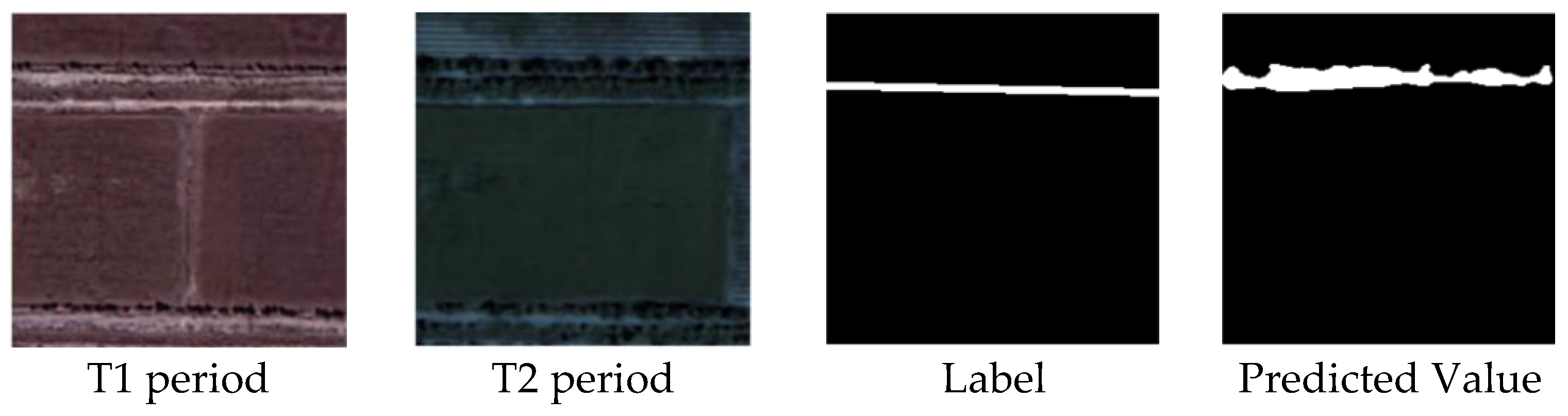
3.2. Experimental Environment and Results

This experiment was conducted on a Windows system, with the hardware environment comprising an Intel Core i7-13650HX CPU, 16 GB RAM, and an NVIDIA GeForce RTX 4060 Laptop GPU (8 GB VRAM). The software environment was based on the deep learning module of ArcGIS Pro 3.0.2, with model training implemented using PyTorch 1.12.1. During training, the batch size was set to 8, and the Adam optimizer was employed with an initial learning rate of 1 × 10⁻⁴, dynamically adjusted according to ArcGIS Pro’s default strategy. Specifically, the learning rate was adapted using an interval slicing strategy, ranging from 2.2908676527677725 × 10⁻⁵ to 0.00022908676527677726 to optimize model convergence. The entire training process was conducted over 200 epochs, and the final trained model parameters were saved for subsequent applications. In the application phase of protective forest change detection, the deep learning inference functionality of ArcGIS Pro was utilized, processing GF-2 remote sensing imagery from 2018 and 2023 with the trained model to detect protective forest changes in the city of Aral. Due to hardware constraints, the remote sensing imagery of Aral was partitioned at the township level, and the 12th regiment town, which exhibited significant changes, was selected as the focal area for analysis. Ultimately, protective forest change detection results for this region were obtained, and a raster map was generated (as shown in Figure 6). Additionally, Figure 7 presents the attribute table of the raster map, detailing information on protective forest changes.

In this study, we conducted a comprehensive and detailed evaluation of the proposed model’s performance in protective forest cover change detection tasks.

Table 1. The experimental results are shown in the figures and tables.

Category	No Change	Change
precision	0.995375	0.785219
Recall	0.939136	0.894787
F1-score	0.966438	0.836430

presents the model’s performance metrics across different categories, including precision, recall, and F1-score, which collectively reflect the model’s reliability and effectiveness in detecting forest cover changes. Additionally, Figure 8 illustrates the practical application of the model, providing a visual representation of the detected forest cover changes for a more intuitive understanding of the results. Specifically, the model demonstrated high precision (0.995375), recall (0.939136), and F1-score (0.966438) for the No Change category, indicating its strong reliability and stability in identifying unchanged areas. However, for the Change category, despite achieving a relatively high recall (0.894787), the model exhibited lower precision (0.785219) and F1-score (0.36430), reflecting an imbalance in detecting changed areas. This imbalance may be attributed to the uneven distribution of samples in the dataset, where unchanged samples dominate, leading to insufficient learning of change features by the model. Additionally, the complexity of change region features and the model’s sensitivity to noise could negatively impact detection accuracy. To enhance the model’s performance in change area detection, future research could employ data augmentation techniques to balance sample distribution, introduce attention mechanisms to improve the capture of change features, and optimize training strategies to address class imbalance issues. These improvements are expected to maintain the high accuracy of the No Change category while significantly enhancing the detection performance of the Change category, thereby better supporting practical applications such as ecological protection and land use monitoring. Furthermore, we conducted an in-depth analysis of the raster attribute table (

Table 2. The attribute table of the Aral City 12th Brigade Protective Forest Change Raster Map.

OID	Value	Class	Red	Green	Blue	Count
1	0	No Change	0	0	0	1,395,979,110
2	255	Change	255	255	255	2,773,666

), which revealed the presence of class imbalance within the dataset. Specifically, the number of pixels in the No Change category (1,395,979,110) was significantly higher than that in the Change category (2,773,666). The proportion of pixels in the Change category was only 0.2% compared to 98.8% in the No Change category. This imbalance may lead the model to favor predicting the No Change category during training, thereby affecting the detection performance for the Change category. In the dataset, the No Change category has a value of 0 and an RGB representation of (0, 0, 0), indicating unchanged areas, while the Change category has a value of 255 and an RGB representation of (255, 255, 255), denoting changed areas. This class imbalance aligns with the lower F1-score (0.3643) observed for the Change category in the model evaluation, further highlighting the challenges faced in detecting change regions. To mitigate this issue, data augmentation techniques could be employed to balance the number of samples, or higher weights could be assigned to the Change category during training to guide the model toward focusing more on changed areas. Additionally, incorporating attention mechanisms or more complex model architectures could enhance the model’s ability to represent change features. In terms of color mapping, the No Change and Change categories are marked in black and white, respectively, which plays a crucial role in visualization and result interpretation. Overall, accurately detecting change regions is critical for ecological protection and land use monitoring. Future studies should further optimize model architectures and training strategies to enhance the detection performance of the Change category, thereby better serving practical application needs.

Buffer analysis is a common geospatial analysis method used to measure the influence range around specific features. In spatial analysis, buffer zones are typically applied to assess environmental impacts, resource distribution, and regional planning. The fundamental principle of buffer analysis involves creating an equidistant zone around point, line, or polygon features within a specified distance, representing the potential impact range of the feature. In this study, buffer analysis was conducted on protective forest change areas to investigate the spatial expansion characteristics of these changes and their impact on the surrounding environment. In ArcGIS Pro, the raster map was first converted into a vector map, and the change category polygon features were extracted to generate buffer zones using the Buffer Analysis tool. The specific parameters were set as follows: the buffer radius was defined as 40 m to ensure coverage of an adequate influence area; the buffer side type was set to FULL, meaning buffers were generated around all feature boundaries; the end type was defined as ROUND, ensuring a smooth buffer boundary; the dissolve type was set to ALL, merging adjacent buffers into a single entity to minimize redundant areas; and the PLANAR method was employed, using Euclidean distance calculations within a projected coordinate system to ensure buffer zone accuracy. Finally, the generated buffer results were overlaid with the raster map to analyze the spatial distribution patterns of protective forest changes, with the results shown in Figure 7.

3.3. Spatial Feature Analysis of Change Detection

3.3.1. Spatial Correlation Analysis

In this study, Global Moran’s I was employed to quantitatively analyze the spatial autocorrelation of protective forest changes in the city of Aral, aiming to explore the spatial patterns of protective forest changes and their potential influencing factors. The analysis results indicate that Moran’s I index is 0.045686, Z-score is 11.809507, and p-value is 0.000000, suggesting a statistically significant positive spatial correlation in protective forest changes. This means that changes in protective forest are spatially similar in adjacent regions rather than being randomly distributed. Although the Moran’s I index (0.045686) is relatively small, the high Z-score (11.809507) and near-zero p-value confirm the presence of significant spatial autocorrelation. This implies that protective forest changes exhibit a certain degree of local clustering rather than random variations, as illustrated in

Table 3. Spatial correlation of protective forest changes in Aral City.

Moran’s I Index	Z-Score	p-Value
0.045686	11.809507	0.000000

, which depicts the spatial correlation of protective forest changes in the city of Aral.

3.3.2. High–Low Clustering

In this study, the General G statistic was used to analyze the spatial clustering characteristics of protective forest changes in the city of Aral, aiming to reveal the spatial distribution patterns of protective forest changes. The results show that the observed value of General G is 0.000145, the expected value is 0.000115, and the variance is close to 0, suggesting that the spatial distribution pattern of the data may not be random. More importantly, the Z-score is 7.900724 and the p-value is 0.000000, indicating that at a 99% confidence level, there is a significant spatial clustering phenomenon in protective forest changes. This means that the protective forest change areas in Aral are not evenly distributed but rather exhibit a high-cluster pattern, as shown in

Table 4. High–low clustering analysis of protective forest change detection in Aral City.

General G	Z-Score	p-Value
0.000145	7.900724	0.000000

, which presents the high–low clustering analysis of protective forest changes in Aral.

The analysis results are of significant guiding value for the protection and management of protective forest. For areas with high clustering of changes, it is important to conduct in-depth analysis to understand the causes of change and implement targeted ecological restoration measures, such as increasing irrigation sources, optimizing the layout of protective forest, and strengthening wind and sand protection. Additionally, remote sensing imagery and field surveys should be combined for dynamic monitoring of protective forest change trends to ensure the effective maintenance of the ecological function of protective forest. Through General G statistics, this study reveals the spatial clustering characteristics of protective forest changes in the Twelve-Group area of Aral, further confirming that protective forest changes are not randomly distributed but influenced by various factors, including water resources, land use, and policies. The research findings provide scientific evidence for protective forest protection and help in formulating more precise ecological restoration and management strategies.

4. Conclusions

Protective forests serve as a crucial component of arid ecosystem systems, playing an irreplaceable role in windbreak and sand fixation, soil quality improvement, and regional microclimate regulation. Additionally, they have profound implications for regional ecological security and sustainable agricultural development. However, due to the intensification of climate change and human activities, the health status and ecological functions of protective forests in arid regions are facing severe challenges. Precisely monitoring the dynamic changes in protective forests and formulating scientifically sound conservation strategies have become urgent issues in the field of ecological research and management.

This study proposes an efficient method for detecting protective forest changes in arid regions, leveraging high-resolution GF-2 remote sensing imagery in conjunction with a Spatiotemporal Attention Neural Network (STANet) model. The primary objective is to enhance the accuracy and reliability of protective forest monitoring in the city of Aral, Xinjiang, China. The results indicate that the integration of STANet’s spatiotemporal attention mechanisms can effectively extract spatiotemporal features from remote sensing data, suppress noise interference, and significantly improve change detection accuracy. Specifically, the Basic Spatiotemporal Attention Module (BAM) and Pyramid Spatiotemporal Attention Module (PAM) embedded in the STANet framework effectively capture protective forest change patterns, achieving an F1-score of 83.64% and an overall accuracy of 78.52%. These findings demonstrate the model’s capability to accurately identify protective forest dynamics, particularly in arid environments, where traditional methods often struggle with complex topography and long-term temporal data analysis.

Further spatial analysis reveals that the spatial distribution of protective forests in Aral has undergone significant changes over the study period, with vegetation coverage declining in certain regions, indicating a trend of protective forest degradation. Statistical analyses using General G and Global Moran’s I indices suggest that protective forest changes exhibit a strong clustering pattern and significant spatial autocorrelation. Notably, in areas with abundant water resources, protective forest recovery shows a pronounced spatial aggregation effect, whereas land use transitions such as the conversion of farmland to wetlands also contribute significantly to protective forest dynamics. These findings highlight that protective forest changes are not randomly distributed but are influenced by multiple factors, including water resource availability, land use modifications, and policy interventions.

Despite the outstanding performance of the STANet model in protective forest change detection, several challenges remain. First, complex topography and extreme climatic conditions may impose higher demands on the model’s generalization ability. Second, processing long-term temporal data requires significant computational resources. Furthermore, dynamic monitoring of protective forest changes still necessitates integration with additional ground truth data to enhance detection accuracy and model robustness. Future research can further refine the STANet model by incorporating multi-source remote sensing data, such as unmanned aerial vehicle (UAV) imagery and Light Detection and Ranging (LiDAR) data, alongside deep spatiotemporal fusion techniques to improve the accuracy and timeliness of protective forest change detection.

In addition, although this study adopted a random sampling approach to divide the dataset into training and validation sets (80% and 20%, respectively) to ensure consistent spatiotemporal distribution, the reuse of sample regions across image tiles may lead to overlaps between the training and validation sets. This means that the test set may not be entirely independent, potentially resulting in an optimistically biased evaluation of model accuracy. As pointed out by Olofsson et al. [32], an ideal accuracy assessment of change detection maps should be conducted using completely independent samples and incorporate uncertainty metrics. While such sampling protocols were not fully adopted in this study, we acknowledge this limitation and recommend that future work adopt fully independent accuracy assessment procedures, such as post-classification stratified sampling and estimation of accuracy uncertainty, as exemplified in Solórzano et al. [33]. Moreover, the raster attribute table analysis revealed a severe class imbalance in the dataset, with 1,395,979,110 pixels labeled as “No Change” and only 2,773,666 pixels labeled as “Change”. This imbalance may have caused the model to focus more on learning features of the dominant class, which in turn affected the precision and F1-score for the “Change” category. To address this issue, future work could introduce data augmentation techniques, employ class-balanced loss functions, and incorporate attention mechanisms or more complex architectures to enhance the model’s capability in identifying changed regions. Accurately detecting change areas remains vital for ecological protection and land use monitoring in arid regions. Addressing these limitations is key to further improving the robustness and applicability of deep learning models for long-term environmental monitoring.

In summary, this study not only introduces an innovative approach for protective forest change monitoring but also provides valuable scientific insights for ecological conservation and sustainable development in Aral, Xinjiang. The STANet model, leveraging spatiotemporal attention mechanisms, proves to be an effective tool for detecting protective forest changes in the complex environmental conditions of arid regions, offering reliable data support for ecological restoration and management. Moreover, this method exhibits strong adaptability to protective forest monitoring in other arid regions, making it a valuable reference for ecological conservation efforts in similar areas. However, the protection and restoration of protective forest is a long-term and systematic endeavor requiring collaborative efforts from governments, research institutions, and society at large. Future strategies should involve a comprehensive set of measures, including enhanced water resource management, optimized land use policies, and increased investment in ecological restoration, to ensure the sustainable development of protective forest. This study provides new theoretical and technical references for the management and restoration of protective forest in arid regions, offering practical value for ecological conservation and sustainable development.

References

- Zalesov, S.; Magasumova, A. Protective Forest Management Problems in Russia. E3S Web Conf. 2021, 258, 08004. [Google Scholar] [CrossRef]
- Accastello, C.; Poratelli, F.; Renner, K.; Cocuccioni, S.; D’amboise, C.J.L.; Teich, M. Risk-based decision support for Protective Forest and natural hazard management. In Protective Forests as Ecosystem-based Solution for Disaster Risk Reduction (Eco-DRR); IntechOpen: London, UK, 2022. [Google Scholar] [CrossRef]
- Kundu, K.; Halder, P.; Mandal, J.K. Change detection and patch analysis of Sundarban Forest during 1975–2018 using remote sensing and GIS Data. SN Comput. Sci. 2021, 2, 364. [Google Scholar] [CrossRef]
- Huang, C.; Song, K. Forest-cover change detection using support Vector Machines. In Remote Sensing of Land Use and Land Cover; Taylor & Francis: Abingdon, UK, 2016; pp. 212–227. [Google Scholar] [CrossRef]
- Huang, L.; Fang, Y.; Zuo, X.; Yu, X. Automatic change detection method of multitemporal remote sensing images based on 2D-Otsu algorithm improved by Firefly algorithm. J. Sens. 2015, 2015, 327123. [Google Scholar] [CrossRef]
- Li, M.; Im, J.; Beier, C. Machine learning approaches for forest classification and change analysis using multi-temporal Landsat TM images over Huntington Wildlife Forest. GIScience Remote Sens. 2013, 50, 361–384. [Google Scholar] [CrossRef]
- Reddy, C.S.; Jha, C.S.; Dadhwal, V.K. Assessment and monitoring of long-term forest cover changes (1920–2013) in Western Ghats biodiversity hotspot. J. Earth Syst. Sci. 2016, 125, 103–114. [Google Scholar] [CrossRef]
- Wessels, K.; Bergh, F.V.D.; Roy, D.P.; Salmon, B.P.; Steenkamp, K.C.; MacAlister, B.; Swanepoel, D.; Jewitt, D. Rapid land cover map updates using change detection and robust random forest classifiers. Remote Sens. 2016, 8, 888. [Google Scholar] [CrossRef]
- Rocha, I. Towards asimov’s psychohistory: Harnessing Topological Data Analysis. artificial intelligence and social media data to forecast societal trends. arXiv 2024, arXiv:2407.03446. [Google Scholar] [CrossRef]
- de Bem, P.; de Carvalho Junior, O.A.; Fontes Guimarães, R.; Trancoso Gomes, R.A. Change detection of deforestation in the Brazilian amazon using landsat data and Convolutional Neural Networks. Remote Sens. 2020, 12, 901. [Google Scholar] [CrossRef]
- Al-Quraishi, A.M.; Gaznayee, H.A.; Crespi, M. Drought trend analysis in a semi-arid area of Iraq based on normalized difference vegetation index. Normalized Difference Water Index and standardized precipitation index. J. Arid. Land 2021, 13, 413–430. [Google Scholar] [CrossRef]
- Xie, G.; Niculescu, S. Mapping and monitoring of land cover/land use (LCLU) changes in the Crozon Peninsula (Brittany. France) from 2007 to 2018 by machine learning algorithms (Support Vector Machine, random forest, and convolutional neural network) and by post-classification comparison (PCC). Remote Sens. 2021, 13, 3899. [Google Scholar] [CrossRef]
- Govedarica, M.; Ristic, A.; Jovanovic, D.; Herbei, M.V.; Sala, F. Object oriented image analysis in remote sensing of forest and Vineyard Areas. Bull. Univ. Agric. Sci. Veter- Med. Cluj-Napoca. Hortic. 2015, 72, 362–370. [Google Scholar] [CrossRef] [PubMed]
- Zhou, W.; Ming, D.; Hong, Z.; Lv, X. Scene division based stratified object oriented remote sensing image classification. In Proceedings of the 2018 Fifth International Workshop on Earth Observation and Remote Sensing Applications (EORSA), Xi’an, China, 18–20 June 2018; pp. 1–5. [Google Scholar] [CrossRef]
- Chen, X.; Zhao, W.; Chen, J.; Qu, Y.; Wu, D.; Chen, X. Mapping large-scale forest disturbance types with multi-temporal CNN framework. Remote Sens. 2021, 13, 5177. [Google Scholar] [CrossRef]
- Chen, P.; Zhang, B.; Hong, D.; Chen, Z.; Yang, X.; Li, B. FCCDN: Feature constraint network for VHR Image Change Detection. ISPRS J. Photogramm. Remote Sens. 2022, 187, 101–119. [Google Scholar] [CrossRef]
- Khusni, U.; Dewangkoro, H.; Arymurthy, A. Urban Area Change Detection with combining CNN and RNN from sentinel-2 Multispectral Remote Sensing Data. In Proceedings of the 2020 3rd International Conference on Computer and Informatics Engineering (IC2IE), Yogyakarta, Indonesia, 15–16 September 2020; pp. 171–175. [Google Scholar] [CrossRef]
- Kotin, K.K.; Kumar, S.; Alabdeli, H.; Kumar, G.R.; Ramachandra, A.C. Transformer encoder and decoder method for forest estimation and change detection. In Proceedings of the 2024 International Conference on Integrated Circuits and Communication Systems (ICICACS), Raichur, India, 23–24 February 2024; pp. 1–4. [Google Scholar] [CrossRef]
- Chen, H.; Song, J.; Han, C.; Xia, J.; Yokoya, N. Changemamba: Remote sensing change detection with spatiotemporal state space model. IEEE Trans. Geosci. Remote Sens. 2024, 62, 4409720. [Google Scholar] [CrossRef]
- Chen, H.; Shi, Z. A spatial-temporal attention-based method and a new dataset for Remote Sensing Image Change Detection. Remote Sens. 2020, 12, 1662. [Google Scholar] [CrossRef]
- Ronneberger, O.; Fischer, P.; Brox, T. U-Net: Convolutional Networks for Biomedical Image Segmentation. In Proceedings of the Medical Image Computing and Computer-Assisted Intervention–MICCAI 2015: 18th International Conference, Munich, Germany, 5–9 October 2015; Lecture Notes in Computer Science. pp. 234–241. [Google Scholar] [CrossRef]
- Peng, D.; Zhang, Y.; Guan, H. End-to-end change detection for high resolution satellite images using improved UNET++. Remote Sens. 2019, 11, 1382. [Google Scholar] [CrossRef]
- Seo, J.; Park, W.; Kim, T. Feature-based approach to change detection of small objects from high-resolution satellite images. Remote Sens. 2022, 14, 462. [Google Scholar] [CrossRef]
- Zhang, H.; Chen, K.; Liu, C.; Chen, H.; Zou, Z.; Shi, Z. CDMamba: Incorporating local clues into mamba for remote sensing image binary change detection. IEEE Trans. Geosci. Remote Sens. 2025, 63, 4405016. [Google Scholar] [CrossRef]
- Brahim, E.; Amri, E.; Barhoumi, W. Enhancing change detection in spectral images: Integration of unet and resnet classifiers. In Proceedings of the 2023 IEEE 35th International Conference on Tools with Artificial Intelligence (ICTAI), Atlanta, GA, USA, 6–8 November 2023; pp. 513–517. [Google Scholar] [CrossRef]
- Zhou, J.; Hao, M.; Zhang, D.; Zou, P.; Zhang, W. Fusion pspnet image segmentation based method for Multi-Focus Image Fusion. IEEE Photonics J. 2019, 11, 1–12. [Google Scholar] [CrossRef]
- Chai, J.X.; Zhang, Y.S.; Yang, Z.; Wu, J. 3D change detection of point clouds based on density adaptive local Euclidean distance. Int. Arch. Photogramm. Remote Sens. Spat. Inf. Sci. 2022, XLIII-B2-2022, 523–530. [Google Scholar] [CrossRef]
- Wu, H.; Huang, H.; Tang, J.; Chen, W.; He, Y. NET greenhouse gas emissions from agriculture in China: Estimation, spatial correlation and Convergence. Sustainability 2019, 11, 4817. [Google Scholar] [CrossRef]
- Kumari, M.; Sarma, K.; Sharma, R. Using Moran.s I and GIS to study the spatial pattern of land surface temperature in relation to land use/cover around a thermal power plant in Singrauli district, Madhya Pradesh, India. Remote Sens. Appl. Soc. Environ. 2019, 15, 100239. [Google Scholar] [CrossRef]
- Glatthorn, J.; Feldmann, E.; Tabaku, V.; Leuschner, C.; Meyer, P. Classifying development stages of primeval European Beech Forests: Is clustering a useful tool? BMC Ecol. 2018, 18, 47. [Google Scholar] [CrossRef] [PubMed]
- Kobayashi, T.; Yamaguchi MAnd Yokoyama, J. Generalized G-inflation: Inflation with the most general second-order field equations. In Towards Ultimate Understanding of the Universe; World Scientific Publishing: Singapore, 2013; pp. 161–169. [Google Scholar] [CrossRef]
- Olofsson, P.; Foody, G.M.; Herold, M.; Stehman, S.V.; Woodcock, C.E.; Wulder, M.A. Good practices for estimating area and assessing accuracy of Land Change. Remote Sens. Environ. 2014, 148, 42–57. [Google Scholar] [CrossRef]
- Solórzano, J.V.; Mas, J.F.; Gallardo-Cruz, J.A.; Gao, Y.; de Oca, A.F.-M. Deforestation detection using a spatio-temporal deep learning approach with synthetic aperture radar and multispectral images. ISPRS J. Photogramm. Remote Sens. 2023, 199, 87–101. [Google Scholar] [CrossRef]