Article

Using Citizen Science Data as Pre-Training for Semantic Segmentation of High-Resolution UAV Images for Natural Forests Post-Disturbance Assessment

by
Kamyar Nasiri
1,*,
William Guimont-Martin
1,
Damien LaRocque
1,
Gabriel Jeanson
1,
Hugo Bellemare-Vallières
1,
Vincent Grondin
1,
Philippe Bournival
2,
Julie Lessard
2,
Guillaume Drolet
2,
Jean-Daniel Sylvain
2 and
Philippe Giguère
1
1
Northern Robotics Laboratory, Université Laval, Québec, QC G1V 0A6, Canada
2
Ministère des Ressources Naturelles et des Forêts, Québec, QC G1P 3W8, Canada
*
Author to whom correspondence should be addressed.
Forests 2025, 16(4), 616; https://doi.org/10.3390/f16040616
Submission received: 27 January 2025 / Revised: 5 March 2025 / Accepted: 17 March 2025 / Published: 31 March 2025

Abstract

:
The ability to monitor forest areas after disturbances is key to ensure their regrowth. Problematic situations that are detected can then be addressed with targeted regeneration efforts. However, achieving this with automated photo interpretation is problematic, as training such systems requires large amounts of labeled data. To this effect, we leverage citizen science data (iNaturalist) to alleviate this issue. More precisely, we seek to generate pre-training data from a classifier trained on selected exemplars. This is accomplished by using a moving-window approach on carefully gathered low-altitude images with an Unmanned Aerial Vehicle (UAV), WilDReF-Q (Wild Drone Regrowth Forest—Quebec) dataset, to generate high-quality pseudo-labels. To generate accurate pseudo-labels, the predictions of our classifier for each window are integrated using a majority voting approach. Our results indicate that pre-training a semantic segmentation network on over 140,000 auto-labeled images yields an F 1 score of 43.74 % over 24 different classes, on a separate ground truth dataset. In comparison, using only labeled images yields a score of 32.45 %, while fine-tuning the pre-trained network only yields marginal improvements ( 46.76 %). Importantly, we demonstrate that our approach is able to benefit from more unlabeled images, opening the door for learning at scale. We also optimized the hyperparameters for pseudo-labeling, including the number of predictions assigned to each pixel in the majority voting process. Overall, this demonstrates that an auto-labeling approach can greatly reduce the development cost of plant identification in regeneration regions, based on UAV imagery.

1. Introduction

Human activities are a major driver of land cover changes in forest ecosystems, impacting ecosystem traits, functions, and services. Climate change exacerbates these effects by influencing reforestation following disturbances, such as logging, fire, or disease, ultimately affecting ecosystem stability and productivity [1,2]. As forests play a vital role in carbon sequestration and biodiversity conservation, ensuring the successful regeneration of post-disturbance zones is crucial for maintaining ecological balance. Accurate monitoring of the diversity of forest species in these zones is essential to anticipate forest recovery and identify areas where regeneration efforts must be prioritized. However, the complexity and dynamic nature of these environments pose challenges to effective management. Advances in computer vision offer a promising avenue for enabling efficient, autonomous, and precise monitoring practices in regeneration zones. Our work targets the problem of plant monitoring in regeneration zones in order to support resource management, guide investment planning, and protect young forested areas.
Every year in Quebec, hundreds of thousands of hectares of forest that have undergone silvicultural interventions or natural disturbances (cutting, planting, fires, epidemics, etc.) need to be monitored. While all Canadian regions experience forest disturbances like fires and logging, forests in Quebec are different from those in the West Coast of Canada and other provinces and territories because of variations in species composition and ecosystem characteristics. Historically, many inventories and field plots were conducted for this purpose. Given the high resources required (labor, time, and costs) and the lack of precision, technologies such as aerial photo interpretation, LiDAR [3], and UAVs have been considered. Despite this, it is challenging to meet monitoring targets. The same area must be monitored more than once and sometimes in a short period, as young forests evolve very quickly. Not monitoring these forests at the right time can compromise the profitability of silvicultural investments (e.g., loss of plantations) and the expected yields of forest stands (e.g., poorly regenerated stands or with undesired species).
Deep learning algorithms can generate detailed maps of species composition and land cover over vast areas [4], typically using satellite or high-altitude aerial images [5,6,7]. However, these types of images lack the details and resolution needed for accurate species identification and consistent microsite characterization across diverse biomes, which is crucial for effective regeneration efforts. Moreover, limited data availability in the study region hinders the training of deep learning algorithms to characterize regeneration zones. UAVs offer a cost-effective solution to collect larger training datasets of detailed high-resolution images in these zones. These images often achieve centimeter-level spatial resolution, capturing fine details of plant structures and allowing for the clear distinction of individual plants, even in densely forested environments. Moreover, the flexibility of UAVs provides access to areas that are otherwise dangerous, difficult to access, or inaccessible for humans, such as dense forest regions.
Despite the advantages that UAVs provide, the complexity of forest ecosystems makes the labeling process time-consuming. Forests are dynamic and diverse environments, covered by overlapping vegetation, varying canopy densities, and different plant species, each with unique shapes and structures. These features make it complicated to accurately identify elements within the images captured by UAVs, and therefore, human labeling is a time-consuming and labor-intensive process. Also, factors such as lighting, seasonal changes, and the presence of non-plant elements add additional complexity to the task.
To mitigate the complex process of manually labeling UAV images, integrating citizen science datasets and leveraging auto-labeling algorithms have proven to be effective solutions [8,9]. Citizen science data, in particular, offer valuable and cost-effective annotations for a wide range of environmental data, including plant categories. Moreover, these datasets are typically very large, which helps address the challenge of having a limited number of annotated data. They are also usually diverse in terms of image resolution, lighting, distance, point of view, etc., making them adaptable to different study cases and providing great generalization for various approaches.
In this study, we leveraged the iNaturalist citizen science dataset [10] to facilitate the training of semantic segmentation networks for plant classification in post-disturbance zones, as depicted in Figure 1. To this effect, a classifier trained on iNaturalist was used to generate pseudo-labels for our UAV images in a moving-window approach [9]. Over 11,000 full-size UAV images were carefully captured at an altitude between 3 and 5 m , with an average Ground Sampling Distance (GSD) of 1.25   m m . This fine level of detail, coupled with a majority voting strategy during pseudo-label generation, greatly improves their accuracy. Indeed, the intricate structure of the leaves is easily discernible at this scale and is comparable to many pictures in iNaturalist. We demonstrate that pre-training on this large-scale dataset of pseudo-labels is so effective that fine-tuning with hand-annotated UAV images only marginally improves performance, i.e., about 3 % pt on F 1 score. These experiments thus show that our approach of data gathering and pseudo-labeling generalizes well despite the domain gap between citizen science datasets and UAV imagery.
In short, our contributions are as follows:
  • A dataset of 11,269 full-size UAV images, called WilDReF-Q, taken at very low altitude and speed, with an average GSD of around 1.25   m m , collected over around 848.6   h a of natural regrowth environments;
  • Accompanying ground truth for 153 cropped images, hand-labeled over 24 classes;
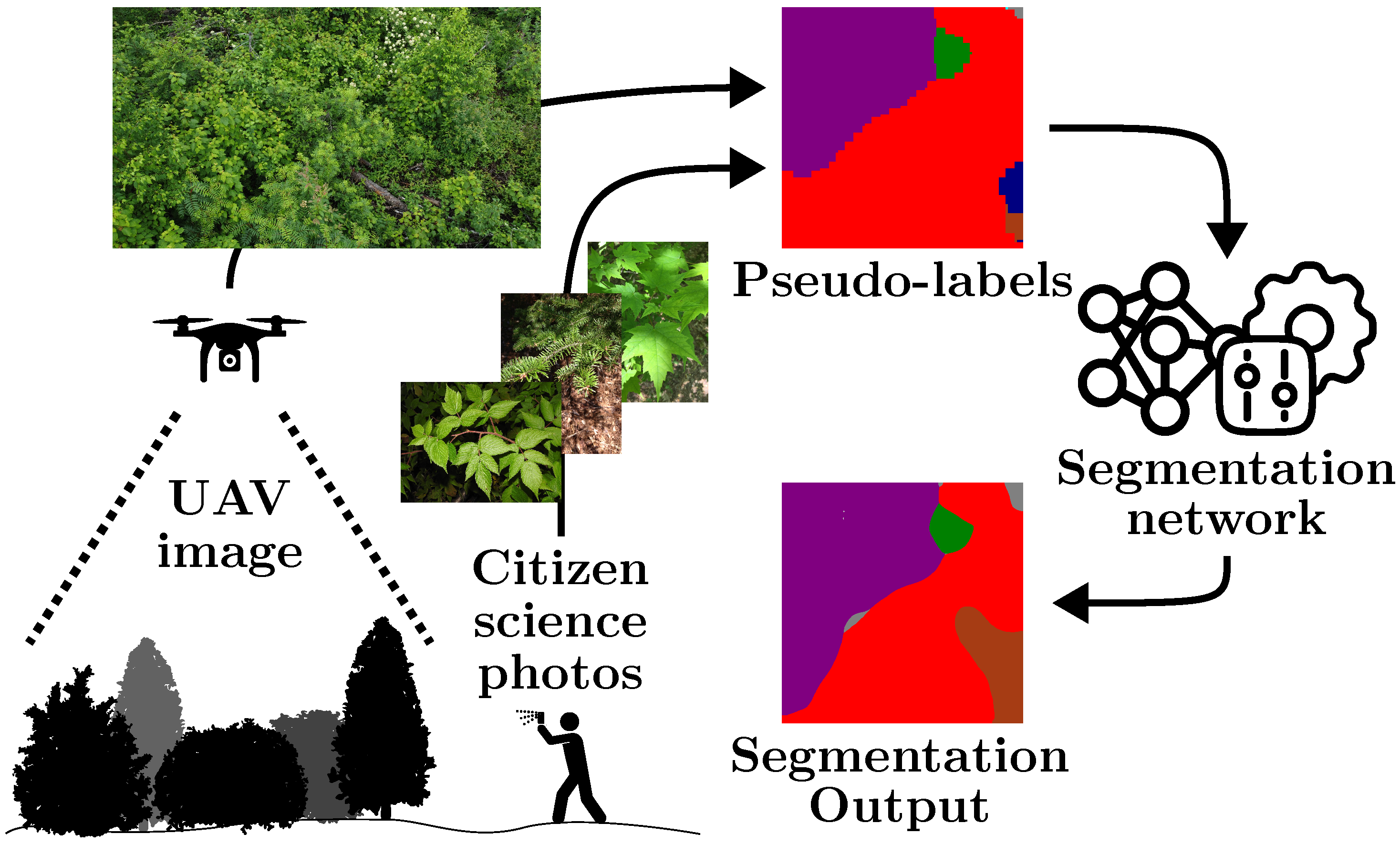
  • Improving the quality of a previous sliding-window pseudo-labeling approach [9], notably by a thorough hyperparameter search and voting over multiple predictions;
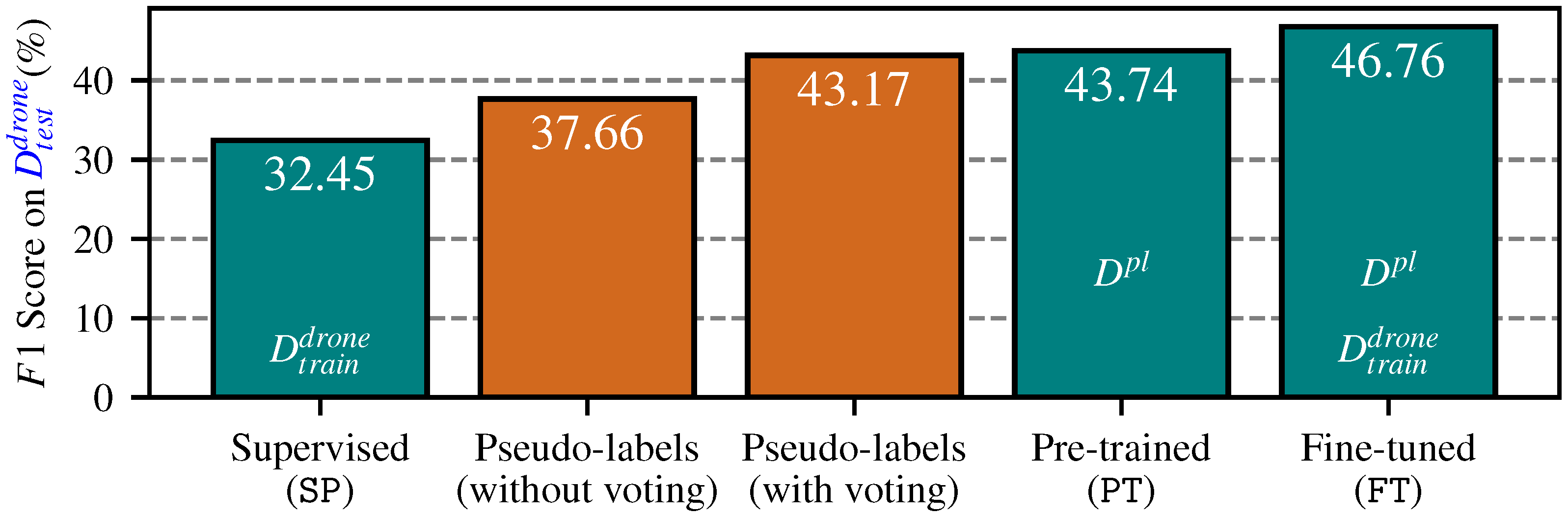
  • Demonstrating that when employed at scale, this pseudo-labeling framework surpasses the use of labeled UAV images.

2. Related Work

2.1. Impact of GSD on UAV Plant Species Mapping

A significant proportion of previous research on plant mapping has focused on UAV surveying at high altitudes (above 30 m ), for which large forested areas must be covered efficiently. Such altitudes have been used to map the Amazonian palm [12], evaluate the impact of autumn leaf phenology on plant mapping [13], and monitor forest health [14]. These altitudes were chosen at the expense of spatial resolution, resulting in fairly large GSD. However, some studies have demonstrated a positive correlation between spatial resolution, i.e., low GSD, and the accuracy of species recognition. For instance, Schiefer et al. [15] demonstrated that the accuracy of forest tree species recognition is superior with images captured at a GSD of 20 m m compared to higher GSDs, with even greater potential for improvement at sub-centimeter resolutions. A study conducted by UAVs in Quebec, Canada, by Jozdani et al. [16], showed the important role of using high-resolution imagery to map caribou lichen, a small plant, over large areas. With a semi-supervised learning approach, they used resampled UAV data with a base GSD of 10 m m to train a network that generated large-scale lichen maps from satellite-scale images, with a coarser GSD of 500 m m . Crown resolution, the ratio of tree-crown size to the number of pixels, was a primary factor considered by Hao et al. [17] in evaluating the performance of Convolutional Neural Network (CNN) models for detecting Chinese fir trees in UAV imagery with a base GSD of 7 m m . They resampled the UAV images at six different resolutions, ranging from 10 m m to 320 m m . Their results showed that increasing spatial resolution generally improved the detection accuracy of the models, except for the finest analyzed resolution (10 m m ). In a similar study by Fromm et al. [18], the average precision of conifer seedling detection improved as the resampled GSD decreased from 63 m m to 3 m m . Gan et al. [19] showed that the performance of the Detectree2 model [20] improves with higher spatial resolution images for detecting tree crowns, while the performance decreased significantly when the GSD exceeded 100 m m . The above studies clearly show the positive impact of high spatial resolution in UAV images for plant identification and mapping. Since our work relies on obtaining the highest possible quality of pseudo-labels for pre-training, we targeted a GSD down to millimeter-level, i.e., 0.8 to 1.7   m m . Our study achieved the finest GSD among all the research reviewed. To obtain this exceptional GSD, we used an advanced UAV flying at altitudes ranging from 3 to 5 m .

2.2. Leveraging Citizen Science Contributions for Species Identification

In recent years, crowdsourced datasets, such as Pl@ntNet [21,22,23] and iNaturalist [11] have emerged and can thus be seen as invaluable resources in biodiversity research. The iNaturalist citizen science project [11], which is central to this work, has over 194 million observations of more than 477,000 species as of June 2024. It provides the largest available biodiversity dataset [24,25]. This is due to the platform’s ease of use, which facilitates contributions from naturalists of all levels [25]. Citizen science datasets thus provide accessible and cost-effective data that help model generalization for projects with limited labeled data. In addition, the platform’s intuitive design simplifies the processes of filtering and downloading observations, which is another reason for making iNaturalist an excellent resource for creating high-quality biodiversity datasets. For example, Soltani et al. [8] trained a classifier network using iNaturalist photographs and generated segmentation maps for aerial images using a moving-window approach. This approach highlights how combining ground-based data with advanced image processing techniques can help reduce the gap between the different scales and viewpoints of ground and aerial images.

2.3. Training Semantic Segmentation Networks Based on Pseudo-Labels

Pseudo-labeling for semantic segmentation has been explored for various applications, including surface crack segmentation [26,27], but far less with UAVs in forestry. One such example is the very recent work of Soltani et al. [9], where they used pseudo-masks over ten species to train a CNN-based segmentation model on an experimental forest plantation [28]. These pseudo-masks were generated by a classifier trained on iNaturalist [24] and Pl@ntNet [22,23], using the moving-window approach introduced by Soltani et al. [8]. They noted that the trained segmentation model had a higher F 1 score compared to the pseudo-masks, highlighting the resilience of neural networks to label noise during training [29].
In parallel to Soltani et al. [9], we explored the use of pseudo-labels generated from a classifier trained with iNaturalist [11] data in the context of pre-training segmentation networks. In our study, we strongly focus on pseudo-label quality, starting from the way we capture UAV images (altitude, speed), all the way to the use of majority voting to reduce pseudo-label noise. A key distinction of our work is the very large number of images in our dataset, WilDReF-Q, as well as their spatial resolution. We collected over 140,000 image crops of 1 MPix from our target environment, which is significantly larger than the dataset used in their study. Moreover, our dataset has a finer GSD, averaging 1.25   m m , which is around 1 m m smaller than that in their study. This allowed for us to capture finer details with greater precision, thus potentially improving the accuracy of classification during the generation of pseudo-labels. Our study examines 24 categories, whereas their work focused on only 11 categories. Additionally, our data collection covers a vast area across the province of Quebec, including different bioclimatic domains. Importantly, our research is conducted in open-set natural forestry areas, where we face significant uncertainty and class imbalance. In contrast, their study is based on a controlled environment, with trees planted in a regular grid. In our pseudo-labeling process, we aggregate multiple predictions to generate accurate pseudo-labels, unlike their study, which performed this step after obtaining outputs from a semantic segmentation network. Furthermore, our optimized implementation for fast pseudo-label generation allows learning at scale, which makes a valuable research viewpoint for more efficient pseudo-labeling methods. Another distinctive aspect of our research is the large hyperparameter search we perform at each stage of the approach to ensure high performance and further differentiate our method from previous work.

3. Materials and Methods

In this study, we address the challenge of training a semantic segmentation network, S M 2 F (based on the Mask2Former architecture [30]), for the target environment of natural regeneration zones, for which there are little-to-no labeled UAV images. The first step was to create a large dataset of UAV images taken over these natural regeneration areas in many distant regions of the Canadian province of Quebec. Importantly, we collected this dataset with the unique particularity that it would exhibit a very small GSD, between 0.8 and 1.7   m m . In parallel, we trained a classification network C D I N O v 2 on a dataset D cls comprising numerous images from iNaturalist, tailored for our target species. Applying this classifier in a moving-window manner on our collected UAV images, we generated pre-training pseudo-labels for the semantic segmentation network S M 2 F . We also performed training experiments on S M 2 F with a few annotated UAV images, both before and after pre-training on our pseudo-labels. Overall, this process is depicted in Figure 2.

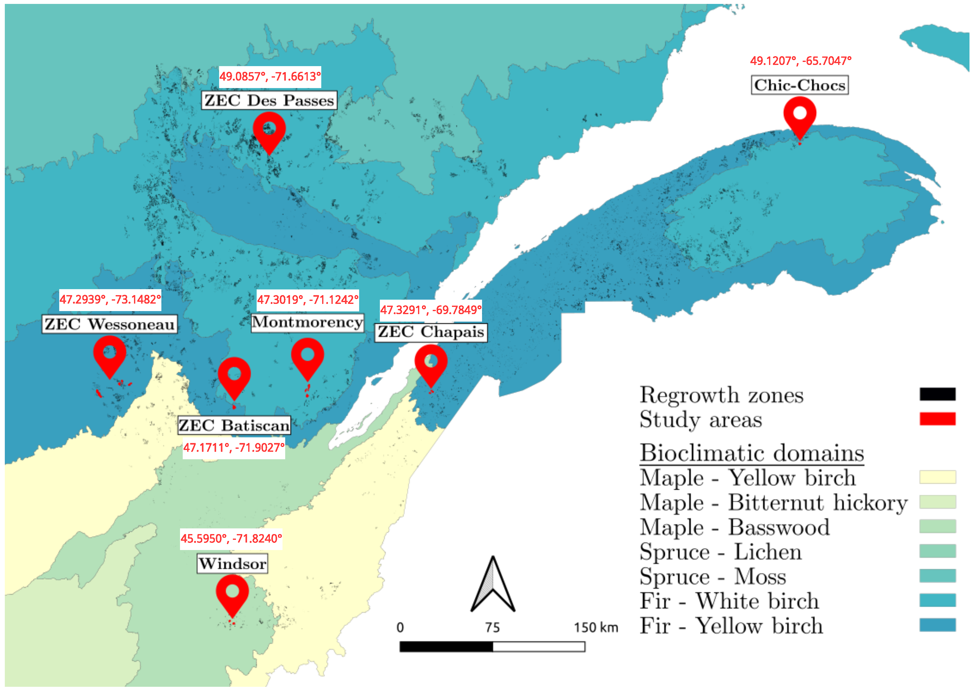
3.1. Areas and Species of Interest

This study was centered on regeneration zones across the province of Quebec, Canada. Specifically, we focused on forest areas that were logged between 2018 and 2022, where vegetation had been growing for two to six years. Figure 3 depicts a map of the southern region of the province of Quebec, where the polygons (black specks) represent regeneration zones, according to geospatial data from the Quebec open data portal [31]. Based on the extracted regeneration polygons, we collected UAV data in seven study sites accross the province, namely ZEC Batiscan (47.1711°, −71.9027°), ZEC Chapais (47.3291°, −69.7849°), Chic-Chocs (49.1207°, −65.7047°), ZEC Des Passes (49.0857°, −71.6613°), Montmorency (47.3019°, −71.1242°), ZEC Wessoneau (47.2939°, −73.1482°), and Windsor (45.5950°, −71.8240°), all shown in Figure 3. They were chosen in a way that ensures the diversity and availability of all target species in our dataset. They also make the segmentation problem much harder compared to using a single site [9], thus are closer to real deployment conditions. The summary of the study sites, presented in Table 1, shows that they are located in three bioclimatic domains of the province of Quebec [32]:
  • Fir/White Birch domain: Located in the southern part of the boreal vegetation zone, this bioclimatic domain is characterized by a dominant presence of fir and white birch trees. The sites in this domain are Montmorency, ZEC Des Passes, and Chic-Chocs.
  • Fir/Yellow Birch domain: Situated in the northern temperate zone’s mixed forest sub-zone, this ecotone marks the transition between the northern temperate and boreal zones. The sites included in this domain are ZEC Wessoneau, ZEC Batiscan, and ZEC Chapais.
  • Maple/Basswood domain: Found in the northern temperate zone’s deciduous forest sub-zone, this domain contains a diverse flora, with many species reaching their northern distribution limits here. The Windsor site represents this domain.
For our study, we targeted 24 classes (20 plants and 4 non-plants) to evaluate the potential for forest restoration after a disturbance. These categories were chosen based on their abundance in the study areas and their impact on the ecosystem [32]. Some target categories included commercially valuable tree species, while others consisted of competitive vegetation or ground obstacles. Some plants, such as spruce trees, are large enough to be identified using a UAV. However, others, such as mosses and ferns, cannot be distinguished at the species level from UAV images. Thus, the target categories include classes at different levels of the taxonomic ranks, as detailed below:
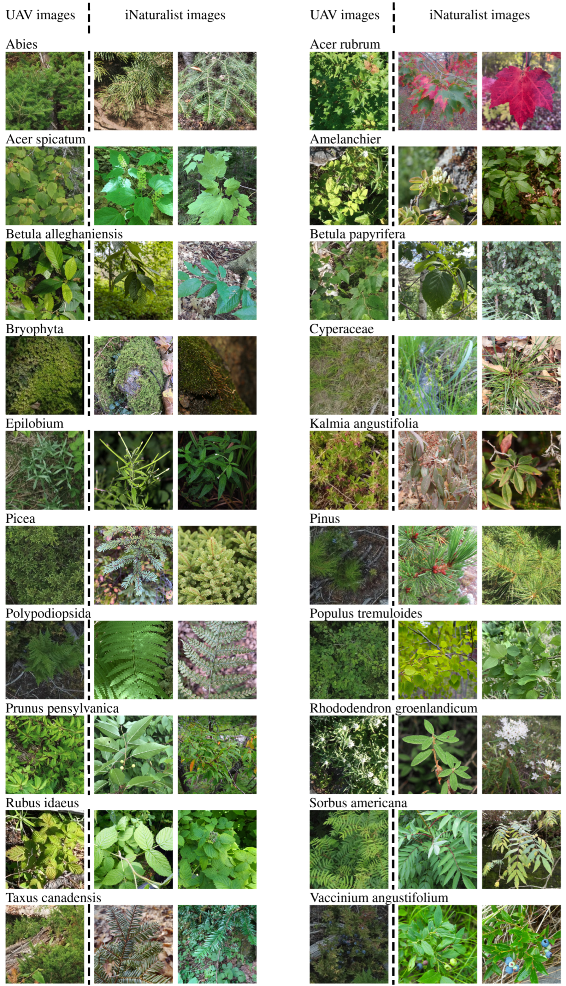
  • Division: Bryophyta (Moss).
  • Class: Polypodiopsida (Fern).
  • Family: Cyperaceae (Sedge).
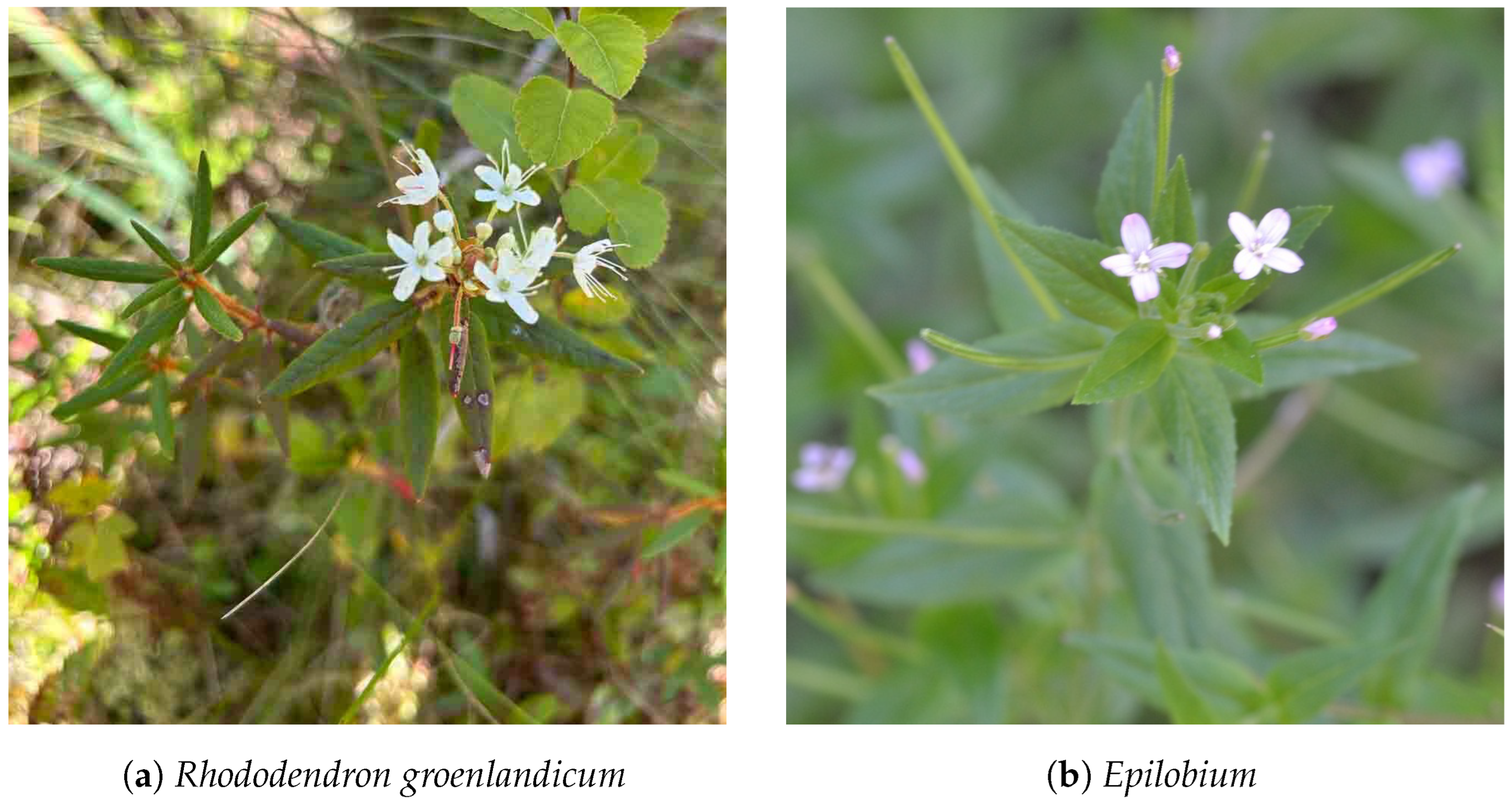
  • Genus: Abies (Fir), Amelanchier (Serviceberry), Epilobium (Willowherb), Picea (Spruce), Pinus (Pine).
  • Species: Acer rubrum (Red Maple), Acer spicatum (Mountain Maple), Betula alleghaniensis (Yellow Birch), Betula papyrifera (Paper Birch), Kalmia angustifolia (Sheep Laurel), Populus tremuloides (Trembling Aspen), Prunus pensylvanica (Fire Cherry), Rhododendron groenlandicum (Bog Labrador Tea), Rubus idaeus (Red Raspberry), Sorbus americana (American Mountain-Ash), Taxus canadensis (Canadian Yew), Vaccinium angustifolium (Lowbush Blueberry).
Due to their visual similarity, particularly in UAV imagery, Moss and Lichen are grouped together and collectively treated as a single class, labeled Moss, in our work. The four remaining non-plant classes are Boulder, Dead Tree, Other, and debriDebris. The Other class encompasses all plants that are not part of the above list. This is also necessary due to the fact that operating in a natural environment means that we are in an open-set scenario, i.e., that some classes are not present in the training set. This represents one of the most challenging scenarios in the field of machine learning [33]. As will be shown later, unsurprisingly, our approach has issues with this Other class.

3.2. UAV Image Acquisition
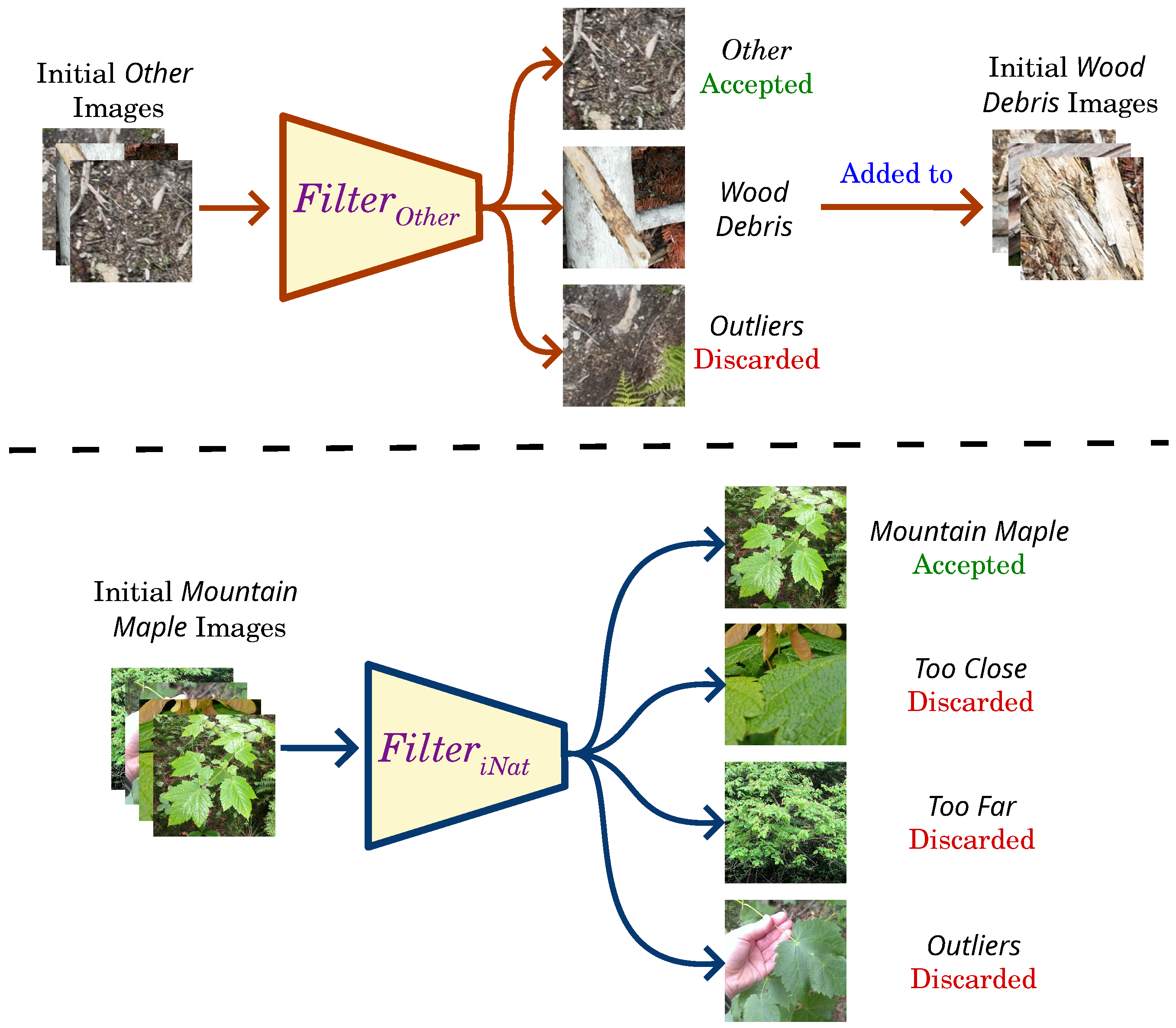
We collected UAV-based RGB images (referred as I drone ) using a DJI Mavic 3 Enterprise (5280 × 3956 pixels, mechanical shutter, FOV = 84°) and a DJI Mini 2 (4000 × 2250 pixels, FOV = 83°). The DJI Mavic 3 Enterprise has a maximum takeoff weight of 1050 g and a flight time of up to 45 min , whereas the takeoff weight of DJI Mini 2 is 246 g and it can fly for a maximum duration of 31 min . The data acquisition parameters were carefully selected to ensure a Ground Sampling Distance (GSD) between 0.8   m m and 1.7   m m . To this end, the surveys were conducted manually at altitudes between 3 to 5 m above the vegetation. The camera settings included ISO values between 100 and 200 and exposure times from 1 / 1000 to 1 / 5000   s , based on lighting conditions. To limit motion blur, the UAV’s velocities were limited to less than 1 m   s 1 . For example, at a typical velocity of 2.5   m   s 1 and shutter speed of 1 / 1000   s , the effective GSD cannot be less than 2.5   m m . The focus was adjusted manually or automatically, depending on the environment’s complexity. Image capture intervals were set to every 5 s for the Mini UAV and every 2 s for the Mavic UAV. Deploying both UAVs at the same time increased the number of pictures taken per sortie. Also, at very low altitudes, the downdraft from the more powerful thrusters of the Mavic UAV sometimes induced leaf fluttering. We thus used the Mini in some situations.
The field survey spanned nine days throughout the summer of 2024, with an average of two hours of data collection per day. In addition, we had access to approximately 400 images collected over seven days during the summer of 2023. We covered 848.6   h a , capturing 11,269 UAV images. These images were collected over a variety of climate and vegetation zones, as illustrated in Figure 3. To ensure uniform image sizes (a requirement for many semantic segmentation networks), we divided each UAV image into 1024 × 1024 pixel crops, referred to as I drone cropped . This process resulted in a total of 143,208 non-overlapping images I drone cropped .
In our study, we annotated only 153 of these I drone cropped images, under the supervision of forestry experts using the Segments.ai platform [34]. Annotating a single image took from 5 to 20 min These annotated images, referred to as D drone , were split into a train set D train drone , a validation set D val drone , and a test set D test drone . The 36 images in D test drone were selected to be as geographically distant as possible from the other images in D train drone and D val drone , as seen in Figure 4. The images in D test drone were also taken in six out of seven study sites to ensure the models can be tested on their generalization capabilities. Other images were split with a ratio of 60:40 between D train drone and D val drone . Except for the S M 2 F segmentation model, in which we use D train drone in the training phase, we use the combined set ( D train , val drone ) as the validation set. A summary of all datasets used in the study is presented in Table 2.

3.3. Training Data D cls for Image Classifier

As in the study by Soltani et al. [9], our pseudo-label generation relies on training the best image classifier possible. To this effect, we first and foremost gathered thousands of images of our target plant species in the iNaturalist database. These images were downloaded using the pyinaturalist Python package (https://pypi.org/project/pyinaturalist/0.19.0, accessed on 7 March 2024), with a focus on Research-grade observations [10,24]. In addition, we further refined our dataset by limiting the number of images for certain categories based on the geographic location of the observations. This step aimed to better represent the Quebec province by prioritizing observations relevant to its local context. This approach was particularly useful for the categories with diversity and extensive global observation records. From the project titled “Trees of the Northeastern United States and Eastern Canada” (Project Number: 91697), which included 1,719,795 observations across 445 species, we extracted images for the following categories: Abies (Fir), Betula alleghaniensis (Yellow Birch), Betula papyrifera (Paper Birch), and Populus tremuloides (Trembling Aspen). Additionally, for the species Acer rubrum (Red Maple), Epilobium (Willowherbs), Kalmia angustifolia (Sheep Laurel), Picea (Spruce), Rhododendron groenlandicum (Bog Labrador Tea), Rubus idaeus (Red Raspberry), and Vaccinium angustifolium (Lowbush Blueberries), we selected observations specifically from the Northeastern United States and Canada region. For Amelanchier (Serviceberry) and Pinus (Pine), observations were restricted to Canada, while Cyperaceae (Sedges) and Polypodiopsida (Ferns) were limited to Quebec. For Acer spicatum (Mountain Maple), Prunus pensylvanica (Fire Cherry), Sorbus americana (American Mountain-Ash), and Taxus canadensis (Canadian Yew), no location filtering was applied. It is important to note that for the Bryophyta (Mosses) division, we limited our queries on the iNaturalist platform to three specific subgroups due to their diversity and the extensive volume of data. These subgroups include the order Hypnales (Feather Mosses), the genus Cladonia (Pixie Cup and Reindeer Lichens), and the genus Sphagnum (Sphagnum Mosses). We restricted the data gathered from these subgroups to the “Northeastern United States and Canada” region, except for the Sphagnum genus, which had no restrictions. It should be mentioned that all images downloaded from iNaturalist are in RGB format, with most downloaded during the summer of 2024.
The iNaturalist database offers a diverse range of images in terms of distance, angle, and viewpoints, and those images can be significantly different from UAV images, as shown in Figure 5. iNaturalist images are ground-based, and subjects are captured from various distances and angles. Because of the diversity of perspectives and viewpoints, those images include close-ups of species’ leaves, as well as broader context shots. On the other hand, UAV images do not have this diversity as every image has a top-down perspective, missing these details, as well as the overall context. Also, the surroundings in iNaturalist photos sometimes include various elements that are not present in UAV images, like human hands. To reduce the gap between UAV images and the iNaturalist dataset, we developed a filtering approach to remove irrelevant data from the iNaturalist images to ensure alignment with our task domain, i.e., similar appearance. Additionally, we leveraged extensive data augmentation techniques during the training of our image classifier, C D I N O v 2 , to bridge the remaining gap. Both of these techniques will be discussed in this section. The gap between the two datasets will be further discussed in Section 5. Hence, to be suitable for our specific task, we implemented a distance-based filtering method, F i l t e r i N a t , inspired by Soltani et al. [8,9]. This allowed us to keep only the pictures that showed significant vegetation coverage, at an appropriate distance, as shown in Figure 6. We used ResNet50 as the backbone of our classifier, a deep CNN commonly used for image classification tasks. ResNet50 was selected because of its easily accessible pre-trained weights and its low memory and computational requirements. Given the primarily strong results, we did not explore additional backbone options. Moreover, this network only has a limited impact on the overall precision of our approach, since a wrongly filtered-in image will not affect the training of the image classifier C D I N O v 2 significantly. Images were classified into four categories, “reasonable distance”, “too far”, “too close”, and “outliers”. A total of 2000 images, equally sampled from all the plant classes, were manually labeled to develop and evaluate this classifier. The model was trained for 100 epochs, with a batch size of 64, with the Adam optimizer. The learning rate was set to 1 × 10 7 . We used cross-entropy as the loss function, as it is appropriate for multi-class classification problems. F i l t e r i N a t had a test accuracy of 76.8 %. Before filtering, the average number of images per class was around 27,000. After applying the filtering approach, we focused on images classified within a “reasonable distance” category, which reduced this average to approximately 12,000 images per class, meaning more than half the images were discarded by the classifier. This shows the diversity and the noise present in unfiltered iNaturalist images.
The data for the Other, Boulder, Wood Debris, and Dead Tree categories were collected from various sources. Specifically, we gathered UAV and smartphone images on the field, obtaining 100,042 images for Other, 767 images for Wood Debris, and 1431 images for Boulder. The UAV images were captured during summer flights on clear, sunny days around noon, ensuring optimal lighting for high-quality image acquisition. Additionally, for the Wood Debris class, we used the BarkNet 1.0 dataset [35], which contains 23,000 cropped images of bark samples from 23 different tree species native to Quebec, Canada. Finally, for the Dead Tree category, we used the Standing Dead Tree Computer Vision Project dataset [36] and cropped the target areas of the images to obtain a total of 114 images.
For the Other images, we implemented a filtering method, F i l t e r O t h e r , classifying each image as either Other, Outliers, or Wood Debris, as shown in Figure 6. This allows us to refine the dataset by removing ambiguous or irrelevant samples and reducing noise in the Other class. At the same time, we added Other images that looked like wood into the Wood Debris class. We implemented F i l t e r O t h e r with EfficientNetV2S as the backbone. We selected EfficientNetV2S for its superior performance in the classification task, outperforming the ResNet50 model in our evaluations. A total of 2000 images were manually labeled to develop and evaluate this classifier. The model was trained with the Adam optimizer for 50 epochs with a batch size of 64, and the learning rate was set to 5 × 10 6 . We used cross-entropy loss. The model had a test accuracy of 81.7 %. After filtering, the Other class was reduced to 39,433 images, as the Wood class increased to 24,554 images.
In the end, the queried iNaturalist images, along with the four described categories, formed the final dataset ( D cls ) used for training our classification network C D I N O v 2 . This dataset contained over 318 k images in total.

3.4. Training of Image Classifier C D I N O v 2

The network C D I N O v 2 is the foundation used to generate pseudo-labels necessary for pre-training our segmentation network S M 2 F . We thus selected a very strong architecture for the classifier, the ViT-L/14 transformer backbone pre-trained with DINOv2 [37] on ImageNet-1K (https://huggingface.co/facebook/dinov2-large-imagenet1k-1-layer, accessed on 1 April 2024). Leveraging large-scale pre-trained models enables the development of methods for generating general-purpose visual features. DINOv2 is one such pre-training approach, employing self-supervised learning on a large curated dataset. It builds on the teacher–student framework and optimizes for transferable visual representations, which is suitable for downstream tasks such as image classification. We modified the final linear layer to output a vector of dimension num_classes=24. The input size of C D I N O v 2 for training was set as 256 × 256. However, inference can be performed at a different input size. We randomly split the entire dataset D cls into training D train cls and validation D val cls sets, using 5-fold cross-validation. Since our goal is to determine how well this classifier works on UAV images, we used the D test drone dataset to report our results. Additionally, to identify the best training choreography for C D I N O v 2 , e.g., data augmentation, we relied on the D train , val drone for model selection.
For all experiments conducted in this paper, we used Python 3.10.12 and PyTorch 2.2.1. For training the C D I N O v 2 , we set the initial learning rate to 1 × 10 5 and employed the AdamW optimizer with the cross-entropy loss function. We then applied a learning rate step decay with a factor of 1 × 10 4 after 3 epochs. Each fold was trained for 5 epochs. With 5-fold cross-validation, this approach resulted in five distinct model weights per experiment, each corresponding to the epoch with the highest accuracy on D val cls . One challenge with the D cls dataset is its class imbalance, i.e., some classes have significantly more images than others. To address this imbalance, we tested the ImbalancedDatasetSampler Python package (https://github.com/ufoym/imbalanced-dataset-sampler, accessed on 1 August 2024). We set its num_samples parameter to 318,265, the number of images in the filtered dataset. We also tested the filtering methods F i l t e r i N a t and F i l t e r O t h e r to evaluate their effect on the results. To improve the generalization capability of our model, we tested multiple combinations of data augmentation techniques. The different combinations tested in five experiments are shown in Table 3. These augmentations were implemented using albumentations library [38] and were used to simulate multiple real-world conditions and distortions commonly encountered in remote sensing imagery. The five experiments all use the same fully filtered dataset, where the iNaturalist images are filtered by F i l t e r i N a t , and the Other images are filtered by F i l t e r O t h e r . Table 4 shows the different filtering and balancing techniques used for each experiment.

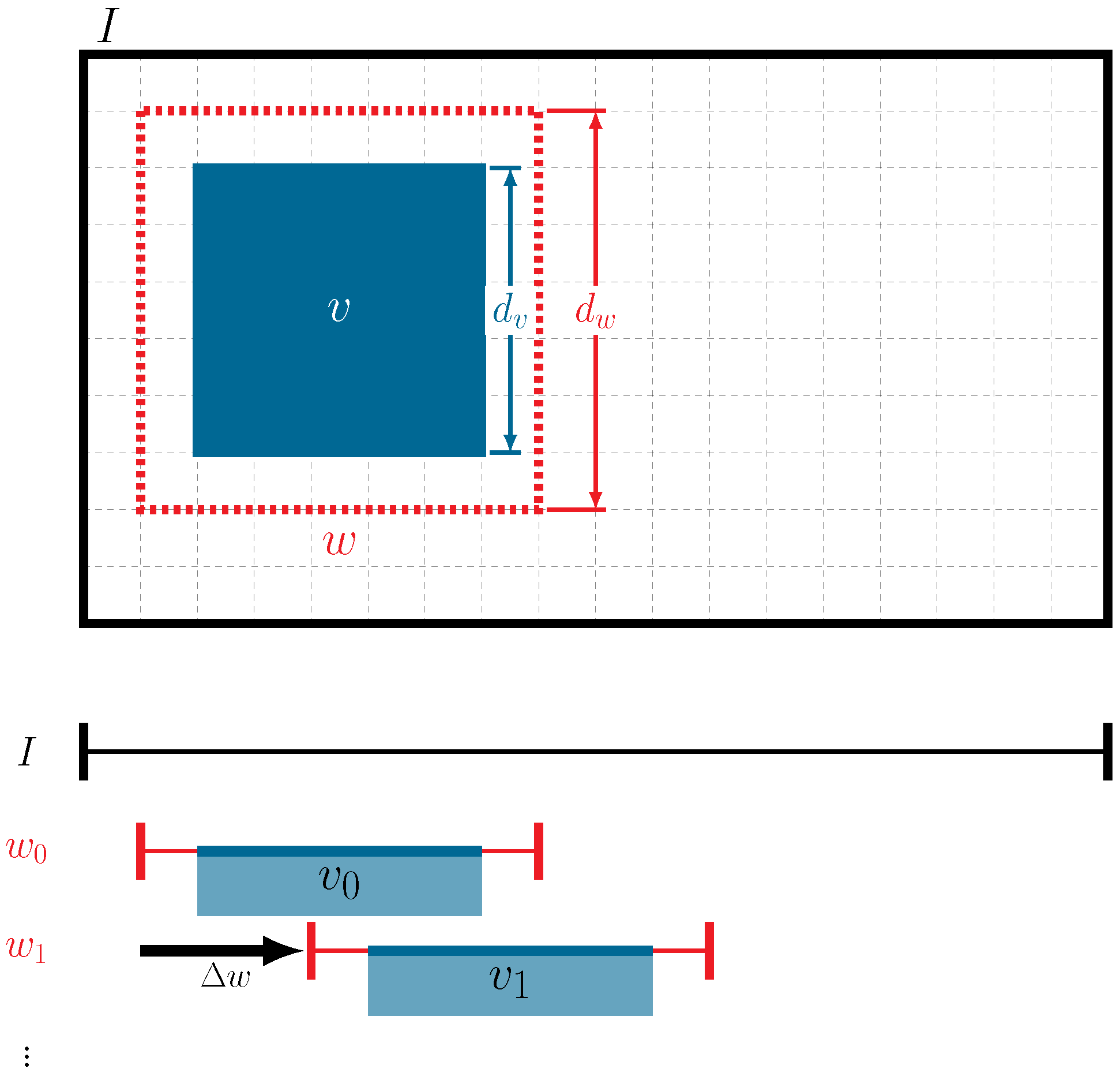
3.5. Generating Pseudo-Labels with a Moving-Window ( I win ) Approach for Pre-Training Data

  To generate the pseudo-labels needed to pre-train the segmentation network S M 2 F , we repeatedly applied the image classifier C D I N O v 2 on smaller crops I win of the 1024 × 1024 UAV images I drone cropped , in a sliding-window approach [9], as depicted in red in Figure 2. The size of I win was an important hyperparameter and was selected using a coarse search, presented in Section 4.1. Conceptually speaking, this window I win should be large enough to contain sufficient information for classification, while small enough so that only one class of vegetation is present most of the time. Unlike Soltani et al. [9], we generate multiple predictions per pixel directly at the pseudo-labeling process of I drone cropped , instead of after the semantic segmentation network. These multiple predictions are aggregated together using a voting strategy, as shown in Figure 7. A voting strategy is especially effective when combining predictions from multiple models or training settings. In our approach, C D I N O v 2 sees each image region multiple times using the sliding-window approach. For each window I win , the classifier generates a prediction, resulting in multiple predictions per region. The final category assigned to each pixel is determined through majority voting, selecting the most frequently predicted class. This allows for a more accurate pre-training dataset, baking the extra precision straight into S M 2 F . The stride Δ w is defined to ensure an overlap ρ , following
Δ w = 1 ρ d v ,
where ρ is the overlap ratio between two consecutive iterations of the moving window and d v is the size of the voting patch.

3.6. Training a Segmentation Model S M 2 F

Semantic segmentation is best executed by a network trained specifically for this task. It allows for much faster inference than any sliding-window method [8], while also taking into account a visual context extending to the whole image (i.e., 1024 × 1024), and not just a smaller window (i.e., 256 × 256). However, training such an end-to-end approach requires a significant amount of labeled data, making this task difficult to apply to novel domains, as in our regeneration zone case. The approach described in Section 3.5 constitutes an efficient way to generate such kind of training data, in the form of our pseudo-labels dataset D pl . Since they have a lower accuracy than carefully hand-labeled examples, they should generally be employed in a pre-training phase. Yet, as we will show in Section 4.3, they can actually surpass a segmentation network trained on ground truth labels, when the latter are in limited amounts. Importantly, the size of this pre-training dataset D pl for semantic segmentation is mostly limited by the capacity to collect data in the field, instead of laborious labeling effort. An experienced UAV operator can collect 300–600 full-size images per hour, which is over 6000 crops of 1024 × 1024 pixels per hour. By comparison, only six such crops can be labeled per hour, if one assumes an average labeling time of 10 min . This 1000× speedup unlocks learning at scale, where the pseudo-labels are generated from as many UAV images as possible. In our work, this is made possible by our pseudo-label generation approach, which is carefully optimized to take less than 5 s to process a 1024 × 1024 image using an NVIDIA RTX-4090 GPU (NVIDIA Corporation, headquartered in Santa Clara, CA, USA). A key benefit of this strategy is that using images from a variety of locations should, theoretically, increase the generalization capability of such a pre-trained network at a minimal cost. In this work, we will compare three different training regimens for S M 2 F : (i) a classical approach where we train only on labeled UAV images D train drone , (ii) only pre-training on D pl to see what kind of performance one can obtain without a single hand-segmented UAV image, and (iii) how much having access to the true labels of D train drone improves a pre-trained model. We selected the segmentation network Mask2Former [30], with a Swin Transformer [39] as a backbone. Mask2Former is a universal architecture to address different segmentation tasks, including semantic segmentation. In this study, Mask2Former is chosen mainly for its ease of use, compatibility with diverse backbone networks, fast convergence, and demonstrated performance on well-known semantic segmentation datasets. Additionally, we show the strengths of Mask2Former by comparing it against U-Net [40], a commonly used semantic segmentation model that was employed in a work similar to ours [9]. U-Net is based on CNNs, with an encoder–decoder architecture.

4. Results

Our experiments were performed along the three main phases of our approach: (i) training the image classifier C D I N O v 2 on D train cls , (ii) generating the pseudo-labels D pl on UAV images with a moving-window I win , and (iii) pre-training our end-to-end segmentation model S M 2 F using these pseudo-labels D pl . To show the effectiveness of our pre-training approach, we fine-tuned a segmentation network on labeled data D train drone , both with and without our pre-training phase.

4.1. Image Classifier C D I N O v 2

After training on D train cls , we tested our classifier on our labeled UAV images D drone . To do so, each UAV image ( I drone cropped ) in D train , val drone or D test drone was divided into patches of size 256 × 256, as is consistent with the input dimensions of D train cls for the image classifier C D I N O v 2 . For this experiment, the patches were extracted with a stride of 256, i.e., with no overlap. Each patch was processed by the C D I N O v 2 image classifier, generating a single prediction. This prediction was then assigned to all the pixels within the corresponding patch. To calculate the F 1 score, we compared the predicted pixel values against the ground truth across each dataset D train , val drone or D test drone individually. We report for both of these datasets, but decisions are taken only based on the results on D train , val drone . Note that there is no data leakage using data flagged as “train” at this step, as these were never actually used to train this classifier: recall that it was trained essentially on curated iNaturalist images, and never on UAV images. We do not report on actual results on the iNaturalist images D cls , as it might not bear much correlation with our task at hand.
In order to obtain a patch classifier generating accurate pseudo-labels, significant efforts were deployed to find the proper training choreography for this image classifier C D I N O v 2 . To this effect, we tested different procedures in the form of ablation studies, as seen in Table 5, and evaluated with the procedure described above. Each of these experiments was performed using a 5-fold cross-validation, with five iterations per fold. Across the five iterations, we selected the best model according to its performance on the iNaturalist images D val cls . One strong factor was the aggressive use of data augmentation, which helped compensate for the fact that images in the D cls dataset are taken at different distances and angles than from a UAV. Our preliminary results showed significant confusion between the Other category and the remaining classes, specifically Wood Debris. To solve this issue, we further split Other images into three classes: Other, Wood Debris, and Outliers, using F i l t e r O t h e r . Another key factor was the use of balancing techniques to mitigate the difficult problem of some classes having much fewer images than others. A lesser factor was filtering the iNaturalist data with F i l t e r i N a t to remove the unrepresentative sample, both based on the quality and the distance [8,9], which did result in a reduction, but of less than 1 % pt on D train , val drone . Nevertheless, this had the important benefit of speeding up training time, reducing it from 17.5   h to 9.5   h for one fold on an NVIDIA RTX-4090 GPU, due to the reduced number of images. Overall, applying all these techniques altogether resulted in an F 1 score improving from 29.59 % to 37.84 % on the D test drone . Results on the D train , val drone also show a similar trend in Table 5. Recall that we used the results on D train , val drone for model selection.

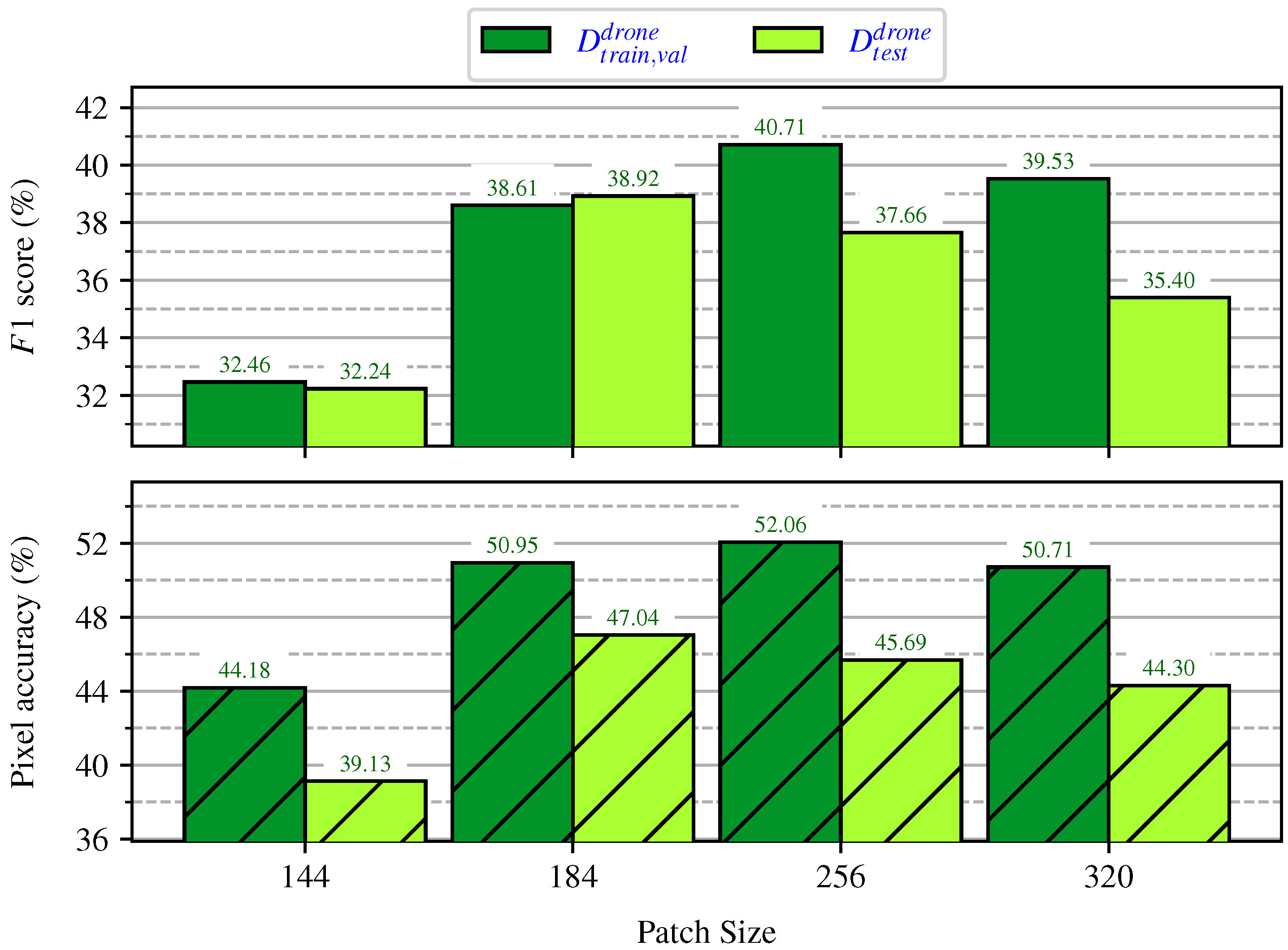
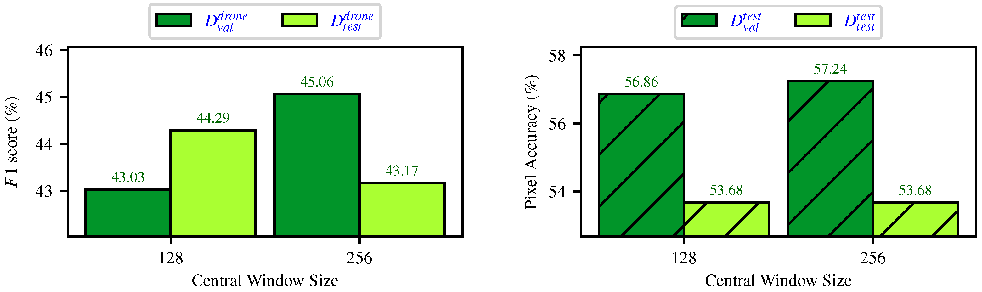
Evaluating the Impact of Patch Sizes on C D I N O v 2 Inference

We tested multiple patch sizes of I drone cropped without overlap to evaluate the performance of C D I N O v 2 across different inference scales. We compare each patch of I drone cropped with the corresponding patch of the ground truth, computing the metrics as explained in Section 4.1. We tested patch sizes of 144, 184, 256, and 320 pixels. The patch sizes were selected based on the experiments to cover from relatively large to relatively small patches. The ViT-L/14 backbone of our classifier C D I N O v 2 is capable of handling different but specific patch sizes, i.e., 150 is not possible. This is due to inherent limitations of vision transformers, namely image tokenization. As shown in Figure 8, the  F 1 score and p A c c were higher with the patch of 256 in validation, so we picked this patch size for future experiments. Here, we solely focus on evaluating the performance of C D I N O v 2 , not of a voting strategy. Hence, we also report the performance of this patch size with the voting strategy in Section 4.2 over pseudo-label generation.

4.2. Pseudo-Label Generation

In this section, we examine different hyperparameters used in the pseudo-label generation process. As discussed in Section 3.5, we investigate the performance of the region of the I win assigned the inferred prediction by the image classifier C D I N O v 2 , and the number of votes tallied to improve pseudo-label accuracy. Based on the performance in C D I N O v 2 inference in Section 4.1, we selected patch sizes of 256. However, since C D I N O v 2 will be used for generating pseudo-labels through an improved process (voting mechanism in Section 4.2.2), it is important to re-evaluate the performance of this I win size. Therefore, as a baseline, we will use a window size of 256 with an overlap of 0.85 and a full window assignment. The  F 1 score achieved is 45.06 % on D train , val drone and 43.17 % on D test drone , compared to 40.71 % on D train , val drone and 37.66 % on D test drone when not using voting.

4.2.1. Impact of Different Prediction Assignments

In this experiment, we investigate the prediction assignment region of each window I win , which means to which pixels the predictions should be propagated to have better performance in the voting method. For instance, propagating the prediction of the image classifier C D I N O v 2 only to the central pixels of a window assumes that this prediction is more correlated to the content in the middle, rather than near its edges. With an I win size of 256, we chose a central size I win central of 128 × 128 (center window assignment) and a central size I win central of 256 × 256 (full window assignment) for comparison. Figure 9 clearly shows that the full window assignment generated better pseudo-labels for D train , val drone . Hence, we will use the full window assignment method to generate pseudo-labels.

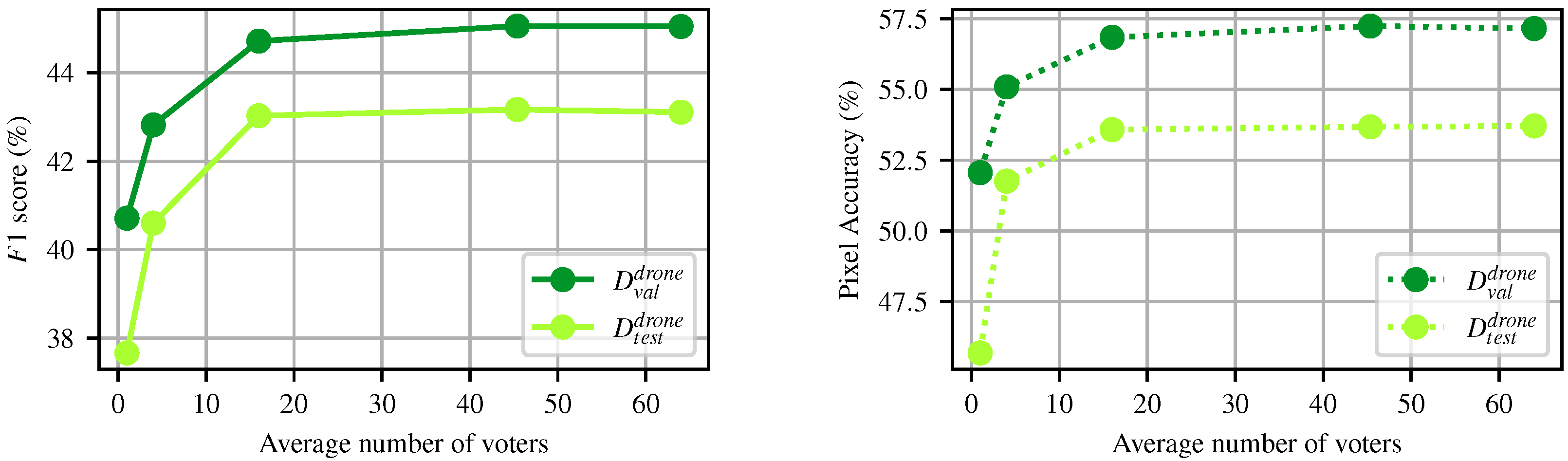
4.2.2. Impact of the Number of Votes

  Collecting predictions for slightly different views is a form of test time augmentation known to increase accuracy [41]. Here, we investigate the impact of using more than one prediction per UAV image pixel, using a majority vote. For this experiment, the size of I win and I win central was set to 256 × 256 pixels. We slid the window by 256, 128, 64, 38 (overlap = 0.85 ), and  32 pixels to gradually increase the number of votes per pixel, as seen in Figure 10. For instance, by sliding by 256 pixels, we only obtain one projected prediction per pixel in I drone cropped , as the pseudo-label generation process of the study by Soltani et al. [8,9]. As expected, we can see that increasing the number of votes per pixel generally increases the F 1 score. In particular, employing 64 votes increases it by 4 % pt , which is a significant improvement. As it exhibited the best results, we selected a pixel stride of 38, resulting in an average of 45.38 votes per pixel.

4.3. End-to-End Segmentation with S M 2 F

We used Mask2Former [30] with a Swin-L backbone [39] as the semantic segmentation network S M 2 F in our experiment. We trained with a learning rate of 1 × 10 4 using the AdamW optimizer. The learning rate scheduler followed a Polynomial decay, with a value of 0.1 for both standard Dropout and DropPath. For data augmentation, we utilized Color Jittering, with saturation and contrast coefficients between 0.8 and 1.2 and a hue shift of 5 degrees. Random horizontal and vertical flips had a probability of 0.5. The batch size was set to 16.
We can clearly see the effectiveness of using the pseudo-labels as pre-training in Figure 11. The standard supervised approach, which only uses the 71 labeled UAV images D train drone , obtains an F 1 score of only 32.45 % over the 24 classes on D test drone . Surprisingly, our 143,055 coarse pseudo-labels of size 1024 × 1024 in D pl already outperform this baseline, even though no human labeling was involved in their generation. These pseudo-labels achieved an F 1 score of 43.17 % on the same test set, D test drone . The segmentation network S M 2 F pre-trained on our pseudo-labels D pl (denoted as PT) raises this score to 43.74 % on D test drone . This improvement of 0.57   % pt over D pl is much less than the 3–6 % pt reported in Soltani et al. [9]. This difference can probably be attributed to the fact that we accrued gains from majority voting in our previous step (pseudo-labeling), as can be seen from the second and third column of Figure 11. In contrast, Soltani et al. [9] performed voting on the semantic segmentation output, thus banking the improvements at this step. Since the gain of S M 2 F (PT) over D pl was very small, multiple S M 2 F were trained to evaluate the results’ variation. We observed that over five experiments, the standard variation is around 1 for the F 1 score on the validation set, showing that the pseudo-labels with voting are statistically indistinguishable to S M 2 F (PT). For completeness, we fine-tuned the pre-trained version of S M 2 F on D train drone (denoted as FT) and achieved an F 1 score of 46.76 %, an increase of only 3.02   % pt over PT. This slight improvement comes at the cost of human labeling, a labor-intensive and costly process. This validates the central point of our work: the vast majority of the performance of S M 2 F comes from our pre-training approach, with modest gain from hand-labeled UAV images. Qualitative results are provided in Figure 12 and Figure 13.
It is important to keep in mind that our problem was significantly more challenging than that of Soltani et al. [9]. First, our number of classes is more than double (24 instead of 11). Second, we dealt with a natural environment, and not planted trees in roughly equal amounts. This implies that we had many species out of distribution, and heavily unbalanced classes in our UAV dataset D drone , as will be discussed in Section 5.
We also compared the performance of using a U-Net [40], as in Soltani et al. [9], to that of a Mask2Former semantic segmentation network. For this, we trained the former using the same pseudo-labels D pl as in the latter. We utilized the U-Net implementation from MMSegmentation [42], an open-source GitHub repository offering multiple implementations of semantic segmentation networks in PyTorch. The network was trained with a learning rate of 1 × 10 4 using the AdamW optimizer for 300,000 iterations. A Polynomial decay learning rate scheduler was applied. For data augmentation, we incorporated photometric distortion with saturation and contrast coefficients ranging from 0.8 to 1.2, along with random horizontal and vertical flips at a probability of 0.5. The batch size was set to 16. This U-Net model achieved an F 1 score of 40.35 % on D test drone . In contrast, as shown in Figure 12 and Figure 13, the Mask2Former S M 2 F trained on the same pseudo-labels achieved an F 1 score of 43.74 % on D test drone . Mask2Former not only achieves a slight improvement over 3 % pt compared to U-Net, but it also demonstrates significantly faster convergence in our experiments.

5. Discussion

In this section, we discuss different aspects of our proposed methodology and results, mentioning both the strengths and weaknesses. We begin by addressing the scalability of our pre-training approach, showing that as the size of our UAV imagery dataset increases, there is a potential for further improvements in performance. Next, we examine the critical role of the small GSD of UAV images in the performance of the classifier, hence in generating pseudo-labels using the moving-window approach. We then present the species distributions across the train, validation, and test sets, and also the generated pseudo-labels. Additionally, we include confusion matrices at each stage of our pipeline to show the classes most often mislabeled over each step. We also discuss several sources of error in our study, such as biases in citizen science data, errors in estimating the GSD, and potential human annotation errors. Finally, we highlight the efficiency of our pseudo-label generation process.
Scaling Data Matters—As part of our experiments, we explored the neural scaling law [43] to evaluate how varying the amount of data in D pl impacts the performance of the pre-training stage (PT) of S M 2 F . As can be seen from Figure 14, the amount of pseudo-labeled pre-training data has a significant impact. The fact that this curve does not exhibit a plateau indicates that collecting more UAV images, which can then be automatically pseudo-labeled, would improve the performance. For reference, we marked the equivalent amount (on a pixel-count basis) of pre-training data available in Soltani et al. [9] with a vertical green dashed line. As can be seen, our study goes almost one order of magnitude farther.
Impact of Ground Sampling Distance (GSD)—Based on our gathered insights from related works, we quickly identified GSD as one of the key parameters to producing more accurate pseudo-labels. Consequently, we selected a very low UAV flight altitude, at 3–5 m above the plants, for our data acquisition sorties. This way, our large unlabeled dataset would contain images capturing many fine vegetation details, especially leaf shape. Our original GSD, ranging from 0.8 to 1.7   m m , also allows us to test this theory, by artificially increasing an image’s GSD via Gaussian blurring. For this test, we were inspired by the Gaussian pyramid approach [44], in which the scaled-down image at level k is obtained by convolving the original image with a Gaussian function. The standard deviation ( σ ) of the Gaussian function is set to 2 k 1 for level k. The increase in the GSD is determined by the downsampling factor. Consequently, convolving the image with a Gaussian function having σ = 2 k 1 ensures that the GSD is proportionally scaled down by a factor of 2 k . We performed this for a factor of 2 over four iterations, resulting in GSD approximate averages of 2.5 , 5.0 , 10.0 , and 20.0   m m , as seen in Figure 15, considering a base average GSD of 1.25   m m .
Although the Gaussian pyramid approach involves downsampling at each stage [44], we chose to exclude the downsampling step in this experiment (both cases are shown in Figure 15). This decision was made to maintain consistent image size I drone cropped and window sizes I win throughout the process, minimizing the impact of varying parameters. Instead, we applied only the Gaussian filter without subsequent downsampling; therefore, we only removed the high-frequency information. In doing so, the conversion to different GSDs in this context represents an approximation of the Gaussian pyramid approach. We believe that this approximation will not affect the ranking shown in Figure 16, especially since, according to the sampling theorem, the blurred data can be optionally represented with fewer samples compared to the original image [45].
As an experiment, we retrained our image classifier, C D I N O v 2 , using the blurred iNaturalist images, providing the instruction explained above. Specifically, before training the new classifiers, we applied Gaussian filter to the iNaturalist data with a standard deviation of σ = 2 k 1 over four iterations. After training the image classifier C D I N O v 2 on the new sets of iNaturalist data, we then evaluated the model on the corresponding blurred annotated test set D test drone to ensure both training and testing were conducted on images with the same level of blur. The results in Figure 16 show that a very fine GSD does not necessarily translate into obtaining better results when performing the pseudo-label generation via the voting strategy. We conjecture that this can be the result of our classifier C D I N O v 2 using data augmentations based on blurring, including MedianBlur and MotionBlur, which makes the model resistant to the blurs we applied. Therefore, the first three models in Figure 16 have all been trained on data with blurs within an approximate similar range. Importantly, images with very fine GSD are necessary for human data annotation, especially in open forest environments. A finer GSD thus enables forestry experts to create more accurate and detailed annotations with greater ease. This is particularly crucial in our case, as our images were acquired over extensive areas with large spacing between them, thus having much less spatial continuity compared to Soltani et al. [9]. This made our annotation a more fastidious task.
Species DistributionFigure 17 illustrates the distribution of species in the pseudo-labels D pl , as well as across the D train , val drone and D test drone datasets. One can see the strong class imbalance present in our problem. While the species distributions in these datasets are not identical, they reflect important differences that can be attributed to the distinct geographic locations where the data were collected. As shown in Figure 4, the annotated data for the training and validation sets were gathered from different locations than the test set, to evaluate the model’s robustness under varying environmental conditions. In addition, it is important to have a test set in which each species is represented with a distribution close to what we see in regeneration forests. The importance is less on the train and validation datasets as a difference in distribution can show the models’ generalization capabilities and avoid over-fitting. Another possible source of label imbalance comes from the fact that our pseudo-labels D pl were generated using the C D I N O v 2 image classifier. This classifier was trained on an imbalanced dataset (iNaturalist), which thus may have introduced biases in the pseudo-labeling generation process, potentially affecting the distribution of species in the resulting labels. For example, Bryophyta (Mosses) was one of the difficult classes to find during UAV data collection since it forms a low-growing, surface-covering layer, often hidden beneath dense vegetation. However, it was one of the most dominant classes in the D train cls training data from iNaturalist. This difference is reflected in the pixel percentage of Bryophyta (Mosses) in the pseudo-labels D pl and the test dataset D test drone , as seen in Figure 17. While there may indeed be more Bryophyta (Mosses) in the unlabeled images D pl , the observed increase is likely inflated due to biases in our C D I N O v 2 classifier.
Confusion Matrix—We present the confusion matrices corresponding to each stage of our pipeline in Figure 18 and Figure 19. These matrices illustrate how our approach reduces confusion and improves results, while also highlighting specific strengths and weaknesses that can guide future work. Importantly, a significant source of confusion arises in predicting the Other class, as seen in Figure 19. This challenge comes from biases in human annotations toward the Other class, particularly in scenes that are complex or difficult to annotate. Examples include environments with extreme shadows or dense vegetation cover, where a human annotator might have used the Other class to signify a lack of clarity. These biases suggest that our annotated training dataset, D train drone , might attribute certain ambiguous features to the Other class. To address this issue, we propose two potential solutions for future work. One is to incorporate a dedicated class for pixels with uncertain predictions that could help mitigate the bias seen in the Other class. The second one is to enhance the pseudo-labeling process by filtering out pixel predictions with low confidence, which would improve the purity of the labels and fine-tuning results. We also noted that our environments’ backgrounds were significantly more complex than the background regions in Soltani et al. [9], as the latter was mostly ground surfaces far away from the canopy presenting a more uniform appearance.
Additionally, the most significant confusion in our pseudo-label generation approach appears to be between Rhododendron groenlandicum (Bog Labrador Tea) and Epilobium (Willowherbs), as is visible in Figure 13. This issue arises mainly because of the overhead viewpoint, which contributes to difficulties in distinguishing between certain species within the genus Epilobium (Willowherbs) and Rhododendron groenlandicum (Bog Labrador Tea), as shown in Figure 20.
Moreover, the Dead Tree class consistently shows poor performance across all stages of our training pipeline (Figure 18 and Figure 19). This issue seems to originate from two challenges. First, the dataset D cls contains only 114 images for the Dead Tree class, which is notably fewer than the other classes. Although we utilize balancing techniques during the classification training of C D I N O v 2 , the large number of samples per epoch significantly exceeds the number of images available for this class. As a result, individual images were repeatedly seen with different augmentations, which limits the model’s ability to generalize effectively. This imbalance highlights the need to prioritize data collection for this class in future work by the UAVs. Second, the Dead Tree class has unique challenges because of its fine shape, making it appear intermingled with other plants. This complexity makes accurate prediction difficult, as shown in Figure 12. Semantic segmentation models often predict contiguous blobs, which further complicates the accurate identification of such small and detailed features. To address this issue, a direction for future work would be training a specialized detector for this Dead Tree class.
Furthermore, we observed poor performance in predicting the Amelanchier (Serviceberry) category. By analyzing the predictions of different stages, i.e., pseudo-label generation, PT, FT, and SP, we identified the main reason: the quality of the UAV annotated images for this class is inferior, and the number of samples in both D train , val drone and D test drone is relatively low. The low quality of the annotated samples mainly comes from issues such as blurriness and shadowy scenes, which we previously discussed. These factors contributed to annotation challenges and detection errors for this category. Importantly, the confusion matrices show that Amelanchier (Serviceberry) is mainly misclassified as Rubus idaeus (Red Raspberry) or the Other category. This confusion is likely due to the poor quality of annotated samples, as Rubus idaeus (Red Raspberry) and Amelanchier (Serviceberry) both belong to the Rose Family (Rosaceae), sharing similar characteristics in their appearance. Additionally, as previously discussed, the Other category includes complex, hard-to-detect scenes and biases in human annotations, further causing these types of errors.
Biases in Citizen Science-Based Datasets—Datasets from citizen science initiatives are inherently biased. For instance, most photos were taken at ground level. This implies that canopies were observed from the bottom, and photos of small plants tend to be very close. Also, there may be a lack of photos of species that are not common in populated areas [46], which could be our situation in post-disturbance zones. Finally, citizen science datasets tend to be biased toward key traits of a species: yellow birch, known for its distinctive bark, is often identified by photos of its trunk rather than by its leaves. This domain gap between citizen science data and UAV images motivated the use of data augmentation and dataset filtering [47].
Identifying the Actual GSD for Manually Driven UAV Data—Since we aimed to capture images with very high spatial resolution, flying the drone at extremely low altitudes was necessary to effectively capture plants in regeneration zones. Flying at such low altitudes involves risks, including potential collisions with taller trees, which makes fully automated flying unsafe. As a result, the drone had to be flown manually, which introduced subtle inconsistencies in estimating the GSD, since the true flight altitude was not known with precision. Additionally, capturing images of taller vegetation led to additional errors in the GSD estimation because of the varying heights of the plants. Despite these challenges, we generally kept a flight altitude of approximately 3 to 5 m above the plants and used these values to estimate the GSD.
Labeling Errors—Manually annotating UAV images of open forest environments presents challenges. This stems from the presence of visually similar plant species, low-quality image sections, partial occlusions by other plants or objects, unknown vegetation, and varying illumination. In our study, we annotated only a limited number of images for inference and fine-tuning, and we ensured that the process was conducted under the supervision of forestry experts. However, in future research, we will expand the annotated dataset to achieve more accurate and diverse inferences. Additionally, we will ensure that potential errors in identifying different plant species are reduced by cooperating with more forestry experts.
Pseudo-Label Generation Speed-Up Process—We sped up the pseudo-labeling process by combining batching, parallelization, and PyTorch’s GPU acceleration, while also utilizing NumPy for efficient grid operations. Batching allowed us to process multiple image patches at once (256 in our experiments), which reduced the overhead and improved throughput. NumPy’s meshgrid was used to efficiently generate pixel offsets for each patch, which is more computationally efficient than doing the same with PyTorch tensors. PyTorch’s mixed-precision with torch.cuda.amp.autocast reduced memory usage and accelerated inference, which made the overall pseudo-label generation process significantly faster.

6. Conclusions

In this study, we explored how a citizen science dataset can be leveraged to train a semantic segmentation network for UAV images. Importantly, it addresses the issue of automated photo interpretation for diverse and complex domains such as forest areas, when faced with little labeled data. To do so, we used a UAV to gather a large-scale dataset, named WilDReF-Q, in natural post-disturbance forest areas. We then developed a procedure to train a moving-window classifier, in order to generate high-quality pseudo-labels at scale, using these collected images.
In terms of datasets, we used iNaturalist data, which included more than 318,000 curated images in 24 categories. These images were used to train our image classification model. The diversity of the data allowed us to train our classifier effectively, despite the domain differences between citizen science images and UAV imagery. To further bridge the gap between these domains, we also employed filtering techniques, different data augmentations, and balancing techniques. We also gathered and curated a UAV dataset, consisting of over 11,000 images captured across different bioclimatic domains in Quebec, Canada. By achieving a GSD between 0.8 and 1.7   m m , these images provided a high level of detail. The annotation of 153 carefully selected image crops by forestry experts provided high-quality ground truth data, which were used as a benchmark for evaluating our models. The large-scale pseudo-labeling process was conducted by our efficient moving-window approach and majority voting strategy, using the classifier trained primarily on iNaturalist data. In order to achieve the best version of generated pseudo-labels, we examined different hyperparameters, such as the number of votes assigned to each pixel in the majority voting approach.
Our experiments have shown that pre-training on these pseudo-labels yields satisfactory results, with subsequent fine-tuning on ground truth data providing only marginal additional benefits. Particularly, pre-training achieved an F 1 score of 43.74 % compared to 32.45 % when trained solely on manually labeled data. Moreover, fine-tuning the pre-trained model with ground truth data improved the performance to 46.76 %. While this result may not be fully suitable for real-world applications, it demonstrates progress compared to previous studies, especially considering the more challenging problem settings and the large number of variant categories involved. We also determined that, based on our results, our approach scales well with the number of unlabeled UAV images. In addition, we demonstrated the impact of millimeter-level GSD images on the generation of accurate pseudo-labels. A significant advantage of our approach is its adaptability, making it easy to add more species to segment or target a different kind of forest area. Indeed, one only has to obtain sufficient exemplar images from iNaturalist, and then reapply the above procedure, which can be fully automated.
Other field surveying and spatial analysis technologies, apart from UAV imagery, have been explored in previous studies. These technologies could be valuable complements to UAV imagery in future research. One such technology is LiDAR [3]. LiDARs provide accurate 3D range information, especially at long distances, but they have lower spatial resolution than cameras. They also lack color or texture data, which are important features in object classification [48]. Additionally, the study by Valjarević et al. [49] used GIS numerical analysis and topographic mapping to assess forest changes in the Toplica region over a 60-year period. This highlights how spatial techniques can enhance the analysis of forest distribution and density.
For future work, we aim to gather additional UAV imagery over the coming years, further pushing in the direction of scale. This expansion will not be limited to the number of images, but will also consider other dimensions, such as capturing data at different times of the year. Building on previous studies [13], we hypothesize that incorporating a multi-seasonal UAV dataset will be advantageous in distinguishing between various plant categories. Collecting data exclusively when the sun is at its nadir can help mitigate the challenges posed by shadowy scenes to ensure more consistent illumination. Additionally, we intend to extend the study to new locations, including a broader range of bioclimatic domains. This will allow us to generalize our findings to more types of forests and geographic regions.
In another aspect of our research, we aim to expand our study to include higher altitude UAV imagery. To achieve this, we propose resampling the fine-resolution, low-altitude images while resampling the segmentation output obtained from the approach of this study as their paired initial masks. These resampled images and masks can be the inputs to train a semantic segmentation network that outputs masks for low spatial resolution images. This could be facilitated by the creation of orthomosaics with a GSD of 1 m m . We plan to employ a tiling approach to generate the orthomosaic, which will help minimize the computational effort required for processing high-resolution data in a single pass. To improve the segmentation accuracy for higher-altitude, lower-resolution imagery, we plan to employ a semi-supervised learning approach. This methodology could potentially refine initial masks, bridge the gap between fine and coarse spatial resolutions, and improve the overall segmentation performance for higher-altitude UAV applications.
Considering our large number of unlabeled images, we plan to explore semi-supervised techniques to improve our workflow. Our approach uses a classifier as a pseudo-label generator with a moving-window strategy. By leveraging a semi-supervised learning method, we aim to refine the classifier masks more effectively. In particular, we will leverage a teacher–student framework where the teacher model generates pseudo-labels for unlabeled images, and the student model is trained using both labeled (classification masks) and pseudo-labeled data. The iterative process will improve the pseudo-labels over time. Additionally, we will use confidence-based filtering to make high-quality pseudo-labels and minimize the confusion between different categories.

Author Contributions

Conceptualization, K.N. and P.G.; methodology, K.N., W.G.-M., D.L., and P.G.; software, K.N., W.G.-M., D.L., G.J., and H.B.-V.; formal analysis, K.N., W.G.-M., D.L., G.J., and P.G.; investigation, K.N., W.G.-M., D.L., G.J., and P.G.; resources, P.G.; data curation, K.N., D.L., G.J., H.B.-V., V.G., and J.L.; writing—original draft preparation, K.N., W.G.-M., D.L., H.B.-V., and P.G.; writing—review and editing, K.N., W.G.-M., D.L., G.J., P.B., J.L., G.D., J.-D.S., and P.G.; visualization, K.N., W.G.-M., D.L., G.J., and V.G.; supervision, P.G.; project administration, P.G.; funding acquisition, P.G. All authors have read and agreed to the published version of the manuscript.

Funding

This research was funded by the Ministère des Ressources naturelles et des Forêts, Contrat 3329-2022-2204-1.

Data Availability Statement

Our dataset (WilDReF-Q) and source code are publicly available online: https://github.com/norlab-ulaval/droneSegmentation (accessed on 1 March 2025).

Acknowledgments

We extend our gratitude to the Ministère des Ressources naturelles et des Forêts of Québec for their invaluable support and guidance. We are deeply appreciative of the contributions of Thomas Careau and Justine Therrien, whose efforts were crucial in the annotation process. Additionally, we gratefully acknowledge the generous support of NVIDIA Corporation for providing an RTX 4090 GPU, which significantly enhanced the computational resources utilized in this research.

Conflicts of Interest

The authors declare no conflicts of interest. The funders had no role in the design of the study; in the collection, analyses, or interpretation of data; in the writing of the manuscript; or in the decision to publish the results.

References

  1. Oliver, T.H.; Isaac, N.J.; August, T.A.; Woodcock, B.A.; Roy, D.B.; Bullock, J.M. Declining resilience of ecosystem functions under biodiversity loss. Nat. Commun. 2015, 6, 10122. [Google Scholar] [CrossRef]
  2. Fassnacht, F.E.; Latifi, H.; Stereńczak, K.; Modzelewska, A.; Lefsky, M.; Waser, L.T.; Straub, C.; Ghosh, A. Review of studies on tree species classification from remotely sensed data. Remote Sens. Environ. 2016, 186, 64–87. [Google Scholar] [CrossRef]
  3. Van den Broeck, W.A.J.; Terryn, L.; Cherlet, W.; Cooper, Z.T.; Calders, K. Three-Dimensional Deep Learning for Leaf-Wood Segmentation of Tropical Tree Point Clouds. Int. Arch. Photogramm. Remote. Sens. Spat. Inf. Sci. 2023, XLVIII-1/W2-2023, 765–770. [Google Scholar] [CrossRef]
  4. Sylvain, J.D.; Drolet, G.; Thiffault, É.; Anctil, F. High-resolution mapping of tree species and associated uncertainty by combining aerial remote sensing data and convolutional neural networks ensemble. Int. J. Appl. Earth Obs. Geoinf. 2024, 131, 103960. [Google Scholar] [CrossRef]
  5. LaRocque, A.; Phiri, C.; Leblon, B.; Pirotti, F.; Connor, K.; Hanson, A. Wetland Mapping with Landsat 8 OLI, Sentinel-1, ALOS-1 PALSAR, and LiDAR Data in Southern New Brunswick, Canada. Remote Sens. 2020, 12, 2095. [Google Scholar] [CrossRef]
  6. Pu, R. Mapping Tree Species Using Advanced Remote Sensing Technologies: A State-of-the-Art Review and Perspective. J. Remote Sens. 2021, 2021, 9812624. [Google Scholar] [CrossRef]
  7. Bolyn, C.; Lejeune, P.; Michez, A.; Latte, N. Mapping tree species proportions from satellite imagery using spectral–spatial deep learning. Remote Sens. Environ. 2022, 280, 113205. [Google Scholar] [CrossRef]
  8. Soltani, S.; Feilhauer, H.; Duker, R.; Kattenborn, T. Transfer learning from citizen science photographs enables plant species identification in UAV imagery. ISPRS Open J. Photogramm. Remote Sens. 2022, 5, 100016. [Google Scholar] [CrossRef]
  9. Soltani, S.; Ferlian, O.; Eisenhauer, N.; Feilhauer, H.; Kattenborn, T. From simple labels to semantic image segmentation: Leveraging citizen science plant photographs for tree species mapping in drone imagery. Biogeosciences 2024, 21, 2909–2935. [Google Scholar] [CrossRef]
  10. iNaturalist Contributors. iNaturalist Research-Grade Observations; iNaturalist Contributors: San Rafael, CA, USA, 2024. [Google Scholar] [CrossRef]
  11. iNaturalist Contributors. iNaturalist. Available online: www.inaturalist.org (accessed on 6 December 2024).
  12. Ferreira, M.P.; Almeida, D.R.A.d.; Papa, D.d.A.; Minervino, J.B.S.; Veras, H.F.P.; Formighieri, A.; Santos, C.A.N.; Ferreira, M.A.D.; Figueiredo, E.O.; Ferreira, E.J.L. Individual tree detection and species classification of Amazonian palms using UAV images and deep learning. For. Ecol. Manag. 2020, 475, 118397. [Google Scholar] [CrossRef]
  13. Cloutier, M.; Germain, M.; Laliberté, E. Influence of temperate forest autumn leaf phenology on segmentation of tree species from UAV imagery using deep learning. Remote Sens. Environ. 2024, 311, 114283. [Google Scholar] [CrossRef]
  14. Ecke, S.; Stehr, F.; Frey, J.; Tiede, D.; Dempewolf, J.; Klemmt, H.J.; Endres, E.; Seifert, T. Towards operational UAV-based forest health monitoring: Species identification and crown condition assessment by means of deep learning. Comput. Electron. Agric. 2024, 219, 108785. [Google Scholar] [CrossRef]
  15. Schiefer, F.; Kattenborn, T.; Frick, A.; Frey, J.; Schall, P.; Koch, B.; Schmidtlein, S. Mapping forest tree species in high resolution UAV-based RGB-imagery by means of convolutional neural networks. ISPRS J. Photogramm. Remote Sens. 2020, 170, 205–215. [Google Scholar] [CrossRef]
  16. Jozdani, S.; Chen, D.; Chen, W.; Leblanc, S.G.; Prévost, C.; Lovitt, J.; He, L.; Johnson, B.A. Leveraging Deep Neural Networks to Map Caribou Lichen in High-Resolution Satellite Images Based on a Small-Scale, Noisy UAV-Derived Map. Remote Sens. 2021, 13, 2658. [Google Scholar] [CrossRef]
  17. Hao, Z.; Lin, L.; Post, C.J.; Mikhailova, E.A.; Yu, K.; Fang, H.; Liu, J. The co-effect of image resolution and crown size on deep learning for individual tree detection and delineation. Int. J. Digit. Earth 2023, 16, 3753–3771. [Google Scholar] [CrossRef]
  18. Fromm, M.; Schubert, M.; Castilla, G.; Linke, J.; McDermid, G. Automated Detection of Conifer Seedlings in Drone Imagery Using Convolutional Neural Networks. Remote Sens. 2019, 11, 2585. [Google Scholar] [CrossRef]
  19. Gan, Y.; Wang, Q.; Iio, A. Tree Crown Detection and Delineation in a Temperate Deciduous Forest from UAV RGB Imagery Using Deep Learning Approaches: Effects of Spatial Resolution and Species Characteristics. Remote Sens. 2023, 15, 778. [Google Scholar] [CrossRef]
  20. Ball, J.G.C.; Hickman, S.H.M.; Jackson, T.D.; Koay, X.J.; Hirst, J.; Jay, W.; Archer, M.; Aubry-Kientz, M.; Vincent, G.; Coomes, D.A. Accurate delineation of individual tree crowns in tropical forests from aerial RGB imagery using Mask R-CNN. Remote Sens. Ecol. Conserv. 2023, 9, 641–655. [Google Scholar] [CrossRef]
  21. PlantNet. With the Pl@ntNet App, Identify One Plant from a Picture, and Be Part of a Citizen Science Project on Plant Biodiversity; PlantNet: Montpellier, France, 2024. [Google Scholar]
  22. Affouard, A.; Goëau, H.; Bonnet, P.; Lombardo, J.C.; Joly, A. Pl@ntNet app in the era of deep learning. In Proceedings of the International Conference on Learning Representations (ICLR), Toulon, France, 24–26 April 2017. [Google Scholar]
  23. Garcin, C.; Joly, A.; Bonnet, P.; Lombardo, J.C.; Affouard, A.; Chouet, M.; Servajean, M.; Lorieul, T.; Salmon, J. Pl@ntNet-300K: A plant image dataset with high label ambiguity and a long-tailed distribution. In Proceedings of the Conference on Neural Information Processing Systems (NeurIPS), Virtual, 6–14 December 2021. [Google Scholar] [CrossRef]
  24. Boone, M.E.; Basille, M. Using iNaturalist to Contribute Your Nature Observations to Science. EDIS 2019, 2019, 5. [Google Scholar] [CrossRef]
  25. Di Cecco, G.J.; Barve, V.; Belitz, M.W.; Stucky, B.J.; Guralnick, R.P.; Hurlbert, A.H. Observing the Observers: How Participants Contribute Data to iNaturalist and Implications for Biodiversity Science. BioScience 2021, 71, 1179–1188. [Google Scholar] [CrossRef]
  26. Konig, J.; Jenkins, M.D.; Mannion, M.; Barrie, P.; Morison, G. Weakly-Supervised Surface Crack Segmentation by Generating Pseudo-Labels Using Localization With a Classifier and Thresholding. IEEE Trans. Intell. Transp. Syst. 2022, 23, 24083–24094. [Google Scholar] [CrossRef]
  27. He, T.; Li, H.; Qian, Z.; Niu, C.; Huang, R. Research on Weakly Supervised Pavement Crack Segmentation Based on Defect Location by Generative Adversarial Network and Target Re-optimization. Constr. Build. Mater. 2024, 411, 134668. [Google Scholar] [CrossRef]
  28. Ferlian, O.; Cesarz, S.; Craven, D.; Hines, J.; Barry, K.E.; Bruelheide, H.; Buscot, F.; Haider, S.; Heklau, H.; Herrmann, S.; et al. Mycorrhiza in tree diversity–ecosystem function relationships: Conceptual framework and experimental implementation. Ecosphere 2018, 9, e02226. [Google Scholar] [CrossRef]
  29. Rolnick, D.; Veit, A.; Belongie, S.; Shavit, N. Deep Learning is Robust to Massive Label Noise. arXiv 2018, arXiv:1705.10694. [Google Scholar] [CrossRef]
  30. Cheng, B.; Misra, I.; Schwing, A.G.; Kirillov, A.; Girdhar, R. Masked-attention Mask Transformer for Universal Image Segmentation. In Proceedings of the IEEE/CVF Conference on Computer Vision and Pattern Recognition (CVPR), New Orleans, LA, USA, 18–24 June 2022. [Google Scholar] [CrossRef]
  31. Ministère des Ressources Naturelles et des Forêts. Récolte et Autres Interventions Sylvicoles, [Jeu de Données]; Ministère des Ressources Naturelles et des Forêts: Québec, QC, Canada, 2017. [Google Scholar]
  32. Ministère des Ressources naturelles et de la Faune. Sustainable Management in the Boreal Forest: A Real Response to Environmental Challenges; Ministère des Ressources naturelles et de la Faune: Québec, QC, Canada, 2008. [Google Scholar]
  33. Zhu, F.; Ma, S.; Cheng, Z.; Zhang, X.Y.; Zhang, Z.; Liu, C.L. Open-world Machine Learning: A Review and New Outlooks. arXiv 2024, arXiv:2403.01759. [Google Scholar]
  34. Segments.ai Team. Segments.ai—The Training Data Platform for Computer Vision Engineers; Segments.ai Team: Leuven, Belgium, 2020; Available online: https://segments.ai (accessed on 15 August 2024).
  35. Carpentier, M.; Giguere, P.; Gaudreault, J. Tree Species Identification from Bark Images Using Convolutional Neural Networks. In Proceedings of the IEEE/RSJ International Conference on Intelligent Robots and Systems (IROS), Madrid, Spain, 1–5 October 2018; pp. 1075–1081. [Google Scholar] [CrossRef]
  36. Standing Dead Tree Computer Vision Project. 2022. Available online: https://universe.roboflow.com/2905168025-qq-com/standing-dead-tree (accessed on 15 July 2024).
  37. Oquab, M.; Darcet, T.; Moutakanni, T.; Vo, H.V.; Szafraniec, M.; Khalidov, V.; Fernandez, P.; HAZIZA, D.; Massa, F.; El-Nouby, A.; et al. DINOv2: Learning Robust Visual Features without Supervision. arXiv 2024, arXiv:2304.07193. [Google Scholar]
  38. Buslaev, A.; Iglovikov, V.I.; Khvedchenya, E.; Parinov, A.; Druzhinin, M.; Kalinin, A.A. Albumentations: Fast and Flexible Image Augmentations. Information 2020, 11, 125. [Google Scholar] [CrossRef]
  39. Liu, Z.; Lin, Y.; Cao, Y.; Hu, H.; Wei, Y.; Zhang, Z.; Lin, S.; Guo, B. Swin Transformer: Hierarchical Vision Transformer using Shifted Windows. In Proceedings of the IEEE/CVF International Conference on Computer Vision (ICCV), Montreal, QC, Canada, 10–17 October 2021; pp. 9992–10002. [Google Scholar] [CrossRef]
  40. Ronneberger, O.; Fischer, P.; Brox, T. U-Net: Convolutional Networks for Biomedical Image Segmentation. In Medical Image Computing and Computer-Assisted Intervention—MICCAI 2015; Springer International Publishing: Berlin/Heidelberg, Germany, 2015; pp. 234–241. [Google Scholar] [CrossRef]
  41. Simonyan, K.; Zisserman, A. Very Deep Convolutional Networks for Large-Scale Image Recognition. In Proceedings of the International Conference on Learning Representations (ICLR), San Diego, CA, USA, 7–9 May 2015. [Google Scholar]
  42. MMSegmentation Contributors. OpenMMLab Semantic Segmentation Toolbox and Benchmark. Apache-2.0 License. 2020. Available online: https://github.com/open-mmlab/mmsegmentation (accessed on 15 November 2024).
  43. Zhai, X.; Kolesnikov, A.; Houlsby, N.; Beyer, L. Scaling Vision Transformers. In Proceedings of the IEEE/CVF Conference on Computer Vision and Pattern Recognition (CVPR), New Orleans, LA, USA, 18–24 June 2022; pp. 1204–1213. [Google Scholar] [CrossRef]
  44. Burt, P.; Adelson, E. The Laplacian Pyramid as a Compact Image Code. IEEE Trans. Commun. 1983, 31, 532–540. [Google Scholar] [CrossRef]
  45. Wandell, B.A. Foundations of Vision; Sinauer Associates: Sunderland, MA, USA, 1995. [Google Scholar]
  46. Piccolo, R.L.; Warnken, J.; Chauvenet, A.L.M.; Castley, J.G. Location biases in ecological research on Australian terrestrial reptiles. Sci. Rep. 2020, 10, 9691. [Google Scholar] [CrossRef]
  47. Ouaknine, A.; Kattenborn, T.; Laliberté, E.; Rolnick, D. OpenForest: A data catalogue for machine learning in forest monitoring. arXiv 2024, arXiv:2311.00277. [Google Scholar] [CrossRef]
  48. Berrio, J.S.; Shan, M.; Worrall, S.; Nebot, E. Camera-Lidar Integration: Probabilistic sensor fusion for semantic mapping. arXiv 2020, arXiv:2007.05490. [Google Scholar]
  49. Valjarević, A.; Djekić, T.; Stevanović, V.; Ivanović, R.; Jandziković, B. GIS numerical and remote sensing analyses of forest changes in the Toplica region for the period of 1953–2013. Appl. Geogr. 2018, 92, 131–139. [Google Scholar] [CrossRef]
Figure 1. An overview of our developed semantic segmentation approach. We leverage citizen science photos to generate pseudo-labels for UAV images. These semantic maps are then further used to train a more accurate segmentation model. Masks are for illustrative purposes only. The citizen science photos are sourced from iNaturalist [11].
Forests 16 00616 g001
Figure 2. Overview of our approach. First, an image classifier C D I N O v 2 is trained on iNaturalist data ( L CLS ), and is used to generate pseudo-labels in a sliding-window fashion. These pseudo-label masks (top-right) are then used to pre-train ( L PT ) a semantic segmentation network S M 2 F , thus reducing greatly the need for hand-labeled images. The pseudo-labels exhibit some granularity due to the scanning window I win size and sliding increment. Moreover, they present significant mistakes: in the shown example, the Forests 16 00616 i001 Prunus pensylvanica is not present in the ground truth, and the Forests 16 00616 i002 
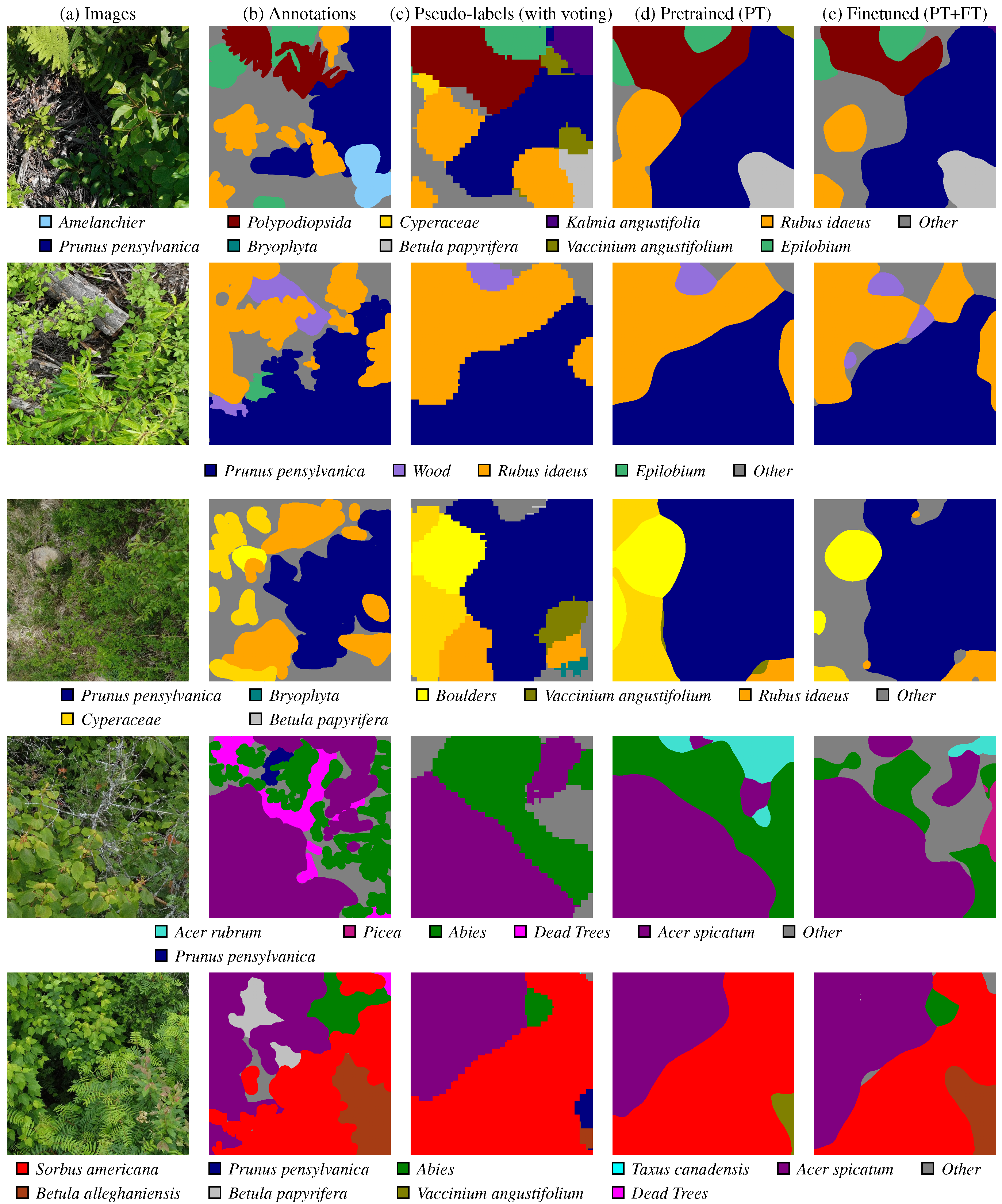
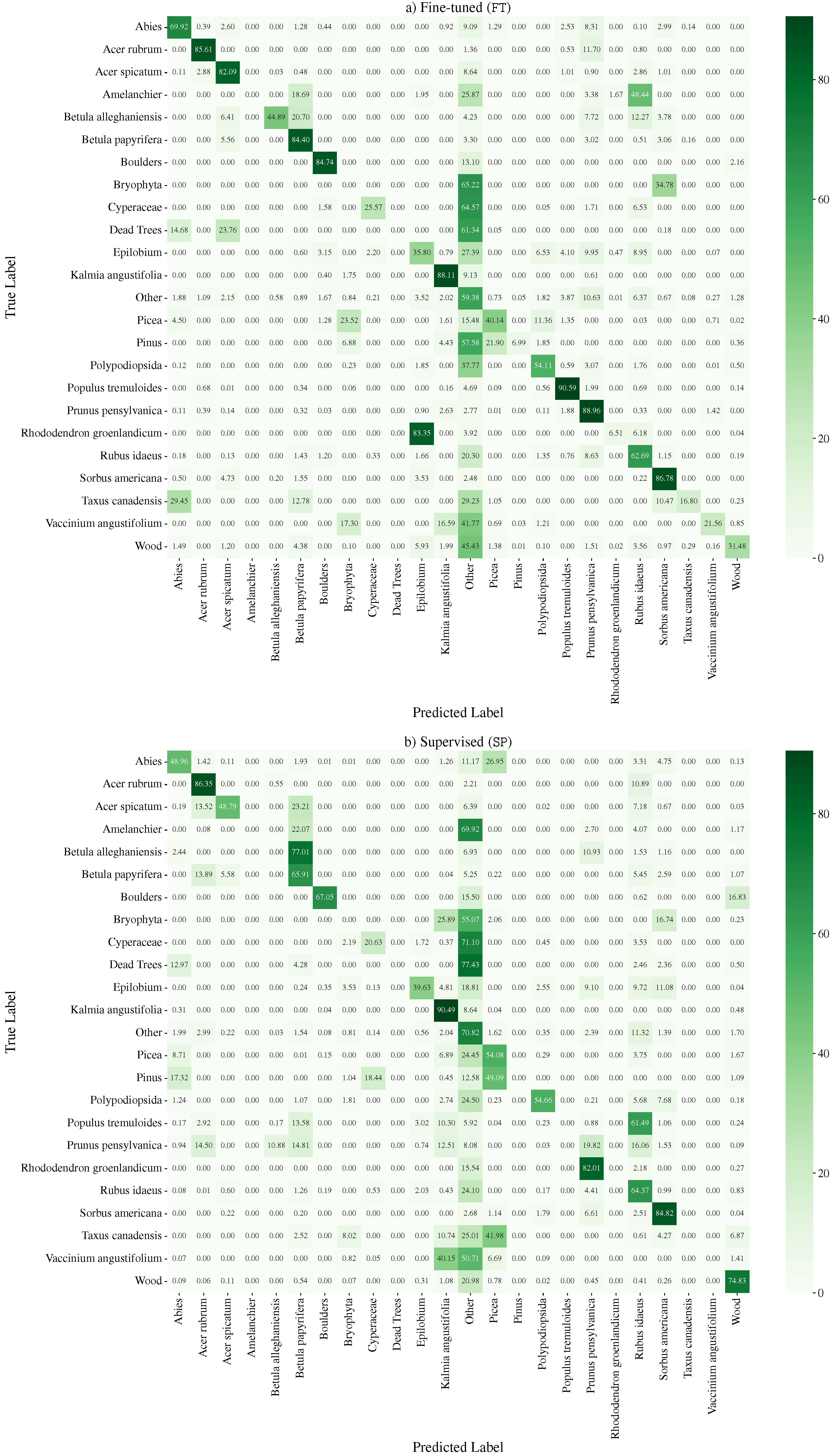
Betula papyrifera is missing. However, the pre-training stage can mitigate some of these pseudo-label mistakes, due to an implicit averaging of labels. It also smooths out the granularity. Finally, fine-tuning ( L FT ) the semantic segmentation network S M 2 F on ground truth annotation provides some, but marginal, improvements. The iNaturalist images are sourced from iNaturalist [10] and the predictions are actual results from our method.
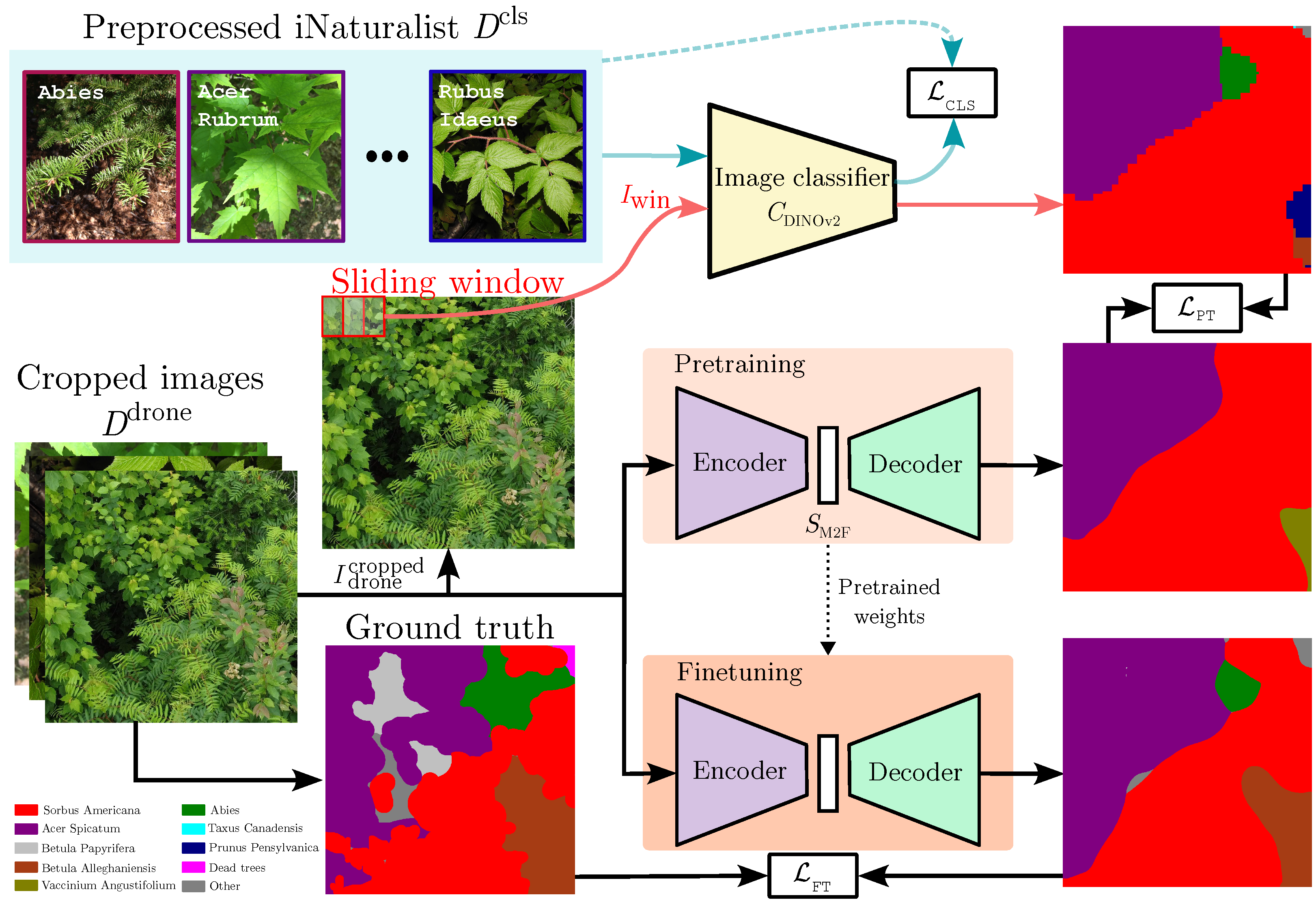
Forests 16 00616 g002
Figure 3. Map of the seven study sites where UAV surveys were conducted. These sites were selected from regeneration zones (black polygons) and cover a range of bioclimatic domains, spanning from the northern temperate forest to the boreal forest in the southern region of the Canadian province of Quebec.
Forests 16 00616 g003
Figure 4. Acquisition location of the train, validation, and test images. The number of images per site is displayed in white text, with a blue background representing the train/validation set and a red background for the test set. The insets show that, for a single study site, the images in the train and validation sets were acquired in different locations than the test images. This clear spatial separation ensures that the model’s generalization capabilities can be properly evaluated.
Forests 16 00616 g004
Figure 5. Differences between iNaturalist ( D cls ) and UAV images ( D drone ) for each of the 20 plant classes.
Forests 16 00616 g005
Figure 6. Classifiers used for D cls filtering. The top classifier was used to filter Other images and remove Outliers and move Wood Debis to the correct class, as the bottom classifier was used to filter iNaturalist plant images by removing Outliers, Too close, or Too far images.
Forests 16 00616 g006
Figure 7. Voting strategy used in the pseudo-labeling process to generate pre-training data for S M 2 F . In this approach, multiple predictions per pixel are made by C D I N O v 2 applied to smaller crops I win of the 1024 × 1024 UAV images I drone cropped . These predictions are aggregated using a voting strategy to improve the accuracy of the pre-training dataset. The stride Δ w defines the shift between consecutive windows, ensuring a specified overlap ratio ρ between them, calculated using Equation (1). The size of the voting patch d v determines the extent of each individual prediction within the sliding window. For instance, in the bottom part of the figure, we can see that some pixels are receiving two votes, v 0 and v 1 .
Forests 16 00616 g007
Figure 8. Classification results of C D I N O v 2 , with different inference patch sizes. We selected 256 as the selected patch size for the pseudo-label generation experiments since it had the highest validation score. Note that we do not perform voting at this stage, which is evaluated separately in Section 4.2. The results reported here represent the performance of the best-performing model from the best fold identified during the 5-fold cross-validation in the final experiment, as detailed in Table 5. The solid bars represent F 1 score, while the hatched bars represent p A c c .
Forests 16 00616 g008
Figure 9. Performance of different central window sizes I win central used for pseudo-label generation. The solid bars represent F 1 score, while the hatched bars represent p A c c .
Forests 16 00616 g009
Figure 10. Pseudo-label generation hyperparameters. Performance of various average number of votes per pixel in I drone cropped . The figure illustrates the performance across average vote counts of 1.0, 4.0, 16.0, 45.38, and 64.0, corresponding to strides of 256, 128, 64, 38, and 32, respectively.
Forests 16 00616 g010
Figure 11. Comparison of F 1 scores on the D test drone dataset across different training methods. The supervised approach (SP) was trained solely on D train drone . Pseudo-labels, both with and without voting, are the result of our pseudo-label generation approach. It is important to note that ‘without voting’ refers to pseudo-label generation with an average of just one voter. The pre-trained model (PT) was only trained on the pseudo-labels D pl . The fine-tuned model (FT) is the PT model fine-tuned on D train drone . Our pre-training approach offers substantial gains in performance.
Forests 16 00616 g011
Figure 12. Qualitative results of our semantic segmentation approach. The pseudo-labels demonstrate excellent predictions, even though the moving-window approach had no exposure to manually labeled data beforehand. Artifacts and square-like boundaries are further refined through the pre-training process, and the results will be enhanced even more through fine-tuning. The first image (from the top) shows significant improvements at each step, while also revealing challenges and inaccuracies in the annotation of Amelanchier (Serviceberry). The second image demonstrates a significant improvement in the prediction for the Wood class in the fine-tuned version. Additionally, the fine-tuned version identified a small piece of wood that was not present in our original annotations. The third sample presents a challenging scene due to a mixture of Cyperaceae (Sedges), Prunus pensylvanica (Fire Cherry), and Rubus idaeus (Red Raspberry), creating complexity for the model in handling dense plant cover. Additionally, the models struggle to differentiate between Cyperaceae (Sedges) and the Other class. The fourth image illustrates how pre-training and fine-tuning refined the boundary between Acer spicatum (Mountain Maple) and Abies (Fir). It also underscores the challenge of accurately predicting rare classes, such as Dead Tree, especially since Dead Trees are often found in complicated shapes, which are difficult to predict. Finally, the fifth sample highlights the difficulty in detecting Betula papyrifera (Paper Birch), which was challenging even for our annotator due to its complete overlap with Acer spicatum (Mountain Maple). Additionally, the models continue to struggle with predicting darker areas in the images, where heavy shadows are present.
Forests 16 00616 g012
Figure 13. More qualitative results are presented in Figure 12. The first image (from the top) illustrates a common misclassification between Rhododendron groenlandicum (Bog Labrador Tea) and Epilobium (Willowherbs). This confusion is since Rhododendron groenlandicum (Bog Labrador Tea) proves particularly challenging to predict, as evidenced by the confusion matrices in Section 5. The second example shows the fine-tuned model’s struggle with darker regions, which points to potential annotation difficulties in the D train drone dataset for pixels with low luminance. This issue is further explored in Section 5. The third image demonstrates significant progress across stages, even with the challenge of dense vegetation coverage. However, fine details remain problematic, particularly with very detailed shapes like Abies (Fir) surrounded by Prunus pensylvanica (Fire Cherry). The fourth example shows the difficulty in scenes dominated by shadows, such as those captured on cloudy days or affected by camera parameters. In these cases, multiple species are often misclassified as Other. Additionally, pseudo-labels and the pre-trained network tend to misidentify dark leaves as Bryophyta (Mosses), likely because of Bryophyta (Mosses) being primarily found on the shadowed ground, which is found in the D train cls training data. Finally, the fifth image illustrates improvements at each stage, particularly in the fine-tuning process, where the Other class is captured with greater precision. Interestingly, the pseudo-labels successfully detect small patches of Epilobium (Willowherb), even in a dense vegetation cover, which shows the model’s potential for handling such complexities.
Forests 16 00616 g013
Figure 14. Impact of pre-training set size on F 1 score. The horizontal lines give the corresponding F 1 scores from Figure 11 for the pseudo-labels with voting and for the supervised model. The vertical line indicates the pixel-count equivalent of the pre-training data used in Soltani et al. [9].
Forests 16 00616 g014
Figure 15. Gaussian filtering applied to a 256 × 256 patch from the D test drone dataset. The first row shows Gaussian blur applied with σ = 2 k 1 at each level of the Gaussian pyramid, where k represents the pyramid level. The second row illustrates Gaussian blur followed by downsampling by a factor of 2 k at each level.
Forests 16 00616 g015
Figure 16. Impact of different Gaussian blur levels (GSDs) on the F 1 score and p A c c of pseudo-labels when training and evaluating on blurred images.
Forests 16 00616 g016
Figure 17. Pixel percentage of each of the 24 classes for the pseudo-labels, D train , val drone and D test drone datasets. It shows the different species distributions in the three datasets, in particular the strong class imbalance.
Forests 16 00616 g017
Figure 18. Confusion matrices for (a) pseudo-label generation using the moving-window approach with the voting strategy, and (b) pre-training (PT) on the generated pseudo-labels using Mask2Former.
Forests 16 00616 g018
Figure 19. Confusion matrices for (a) our fine-tuning approach (FT) applied to the pre-trained weights from the PT stage using 71 annotated images with Mask2Former, and (b) the supervised approach (SP) using 71 annotated images with Mask2Former.
Forests 16 00616 g019
Figure 20. Similarity between the classes Rhododendron groenlandicum (Bog Labrador Tea) and Epilobium (Willowherbs). Certain species within the genus Epilobium (Willowherbs), such as Epilobium ciliatum (Fringed Willowherb), show some similarities to Rhododendron groenlandicum (Bog Labrador Tea) in flower color and leaf shape from an overhead UAV viewpoint. These similarities provided confusion during the pseudo-label generation evaluation on D test drone . Source: iNaturalist images [11].
Forests 16 00616 g020
Table 1. Bioclimatic domains and vegetation zones of each study site [32]. Elevation ( m ) of study sites approximately estimated using online sources. (Estimated based on data from https://en-gb.topographic-map.com, accessed on 2 March 2025, and https://whatismyelevation.com, accessed on 2 March 2025). Figure 3 gives the location of the study sites in the southern part of the Canadian province of Quebec.
SiteVegetation ZoneSub-ZoneBioclimatic DomainElevation
ZEC BatiscanNorthern temperateMixedFir/Yellow Birch550 m
ZEC ChapaisNorthern temperateMixedFir/Yellow Birch350 m
Chic-ChocsBorealContinuousFir/White Birch600 m
ZEC Des PassesBorealContinuousFir/White Birch300 m
MontmorencyBorealContinuousFir/White Birch700 m
ZEC WessoneauNorthern temperateMixedFir/Yellow Birch400 m
WindsorNorthern temperateDeciduousMaple/Basswood250 m
Table 2. Summary of all datasets in this study.
DatasetCountImage Size ( Px ) Description
D cls 318kvariableAggregated citizen science and other
images to train C D I N O v 2
I drone 11,26920 MPix or 9 MPixRaw UAV images
I drone cropped 143,208 1024 × 1024 UAV image crops
D drone 153 1024 × 1024 Annotated UAV image crops
Table 3. Augmentation strategies applied in each experiment. Each row corresponds to a specific data augmentation technique, while each column (labeled 0 to 5) represents a distinct experimental configuration. This table highlights the incremental inclusion and variation of augmentations across experiments to study their individual and combined impacts.
AugmentationExperiments
Aug 0 Aug 1 Aug 2 Aug 3 Aug 4
SmallestMaxSize
RandomResizedCrop
HorizontalFlip
ColorJitter
Blur
ShiftScaleRotate
Perspective
MotionBlur
MedianBlur
OpticalDistortion
GridDistortion
Defocus
RandomFog
Legend: ●: Augmentation applied; ○: Augmentation not applied; ◐ and ◑: Alternating between MotionBlur and MedianBlur; ◓ and ◒: Alternating between OpticalDistortion and GridDistortion.
Table 4. Filtering and balancing techniques applied in different experiments to find the best dataset to use for pseudo-label generation. Each row corresponds to a specific filtering or balancing technique, while each column represents an experiment or a group of experiments. This table highlights the incremental use of filtering and balancing techniques.
TechniqueExperiments
Unfiltered iNaturalist Filtered Fully Filtered Augmentations Balance Final
F i l t e r i N a t
F i l t e r O t h e r
ImbalancedDatasetSampler
Legend: ●: Technique exists in the experiment; ○: Technique does not exist in the experiment.
Table 5. Classification results of C D I N O v 2 , with an inference patch size of 256. The details of data and approaches used for each technique are presented in Table 3 and Table 4. Combining all the techniques resulted in the highest performance, increasing the F 1 score by 13.70   % pt on D train , val drone . The mentioned variations in the table are in comparison with the first experiment (unfiltered baseline). The results reported here represent the average performance of the best model from each fold in the 5-fold cross-validation.
Experiment D train , val drone ( F 1 ) D test drone ( F 1 )
Unfiltered baseline24.93% 29.59%
Filtering technique
iNaturalist filtered24.37% ↓ −0.56 %pt27.26% ↓ −2.32 %pt
Fully filtered34.17% ↑ 9.24 %pt34.12% ↑ 4.53 %pt
Balancing technique
Balance34.23% ↑ 9.31 %pt34.04% ↑ 4.46 %pt
Augmentation technique
Aug 034.40% ↑ 9.48 %pt37.34% ↑ 7.76 %pt
Aug 135.12% ↑ 10.19 %pt36.53% ↑ 6.94 %pt
Aug 235.80% ↑ 10.87 %pt37.13% ↑ 7.54 %pt
Aug 336.29% ↑ 11.36 %pt37.83% ↑ 8.24 %pt
Aug 436.64% ↑ 11.71 %pt36.81% ↑ 7.22 %pt
Final (Balance + Aug 4)38.63% ↑ 13.70 %pt37.84% ↑ 8.25 %pt
Disclaimer/Publisher’s Note: The statements, opinions and data contained in all publications are solely those of the individual author(s) and contributor(s) and not of MDPI and/or the editor(s). MDPI and/or the editor(s) disclaim responsibility for any injury to people or property resulting from any ideas, methods, instructions or products referred to in the content.

