
Climate Effects on Phenology of Two Deciduous Forest Species Across Southern Europe


Abstract
1. Introduction
2. Materials and Methods
2.1. Species and Study Sites
2.2. Satellite Data
2.3. Phenology
2.4. Meteorological Data
2.5. Statistics
3. Results
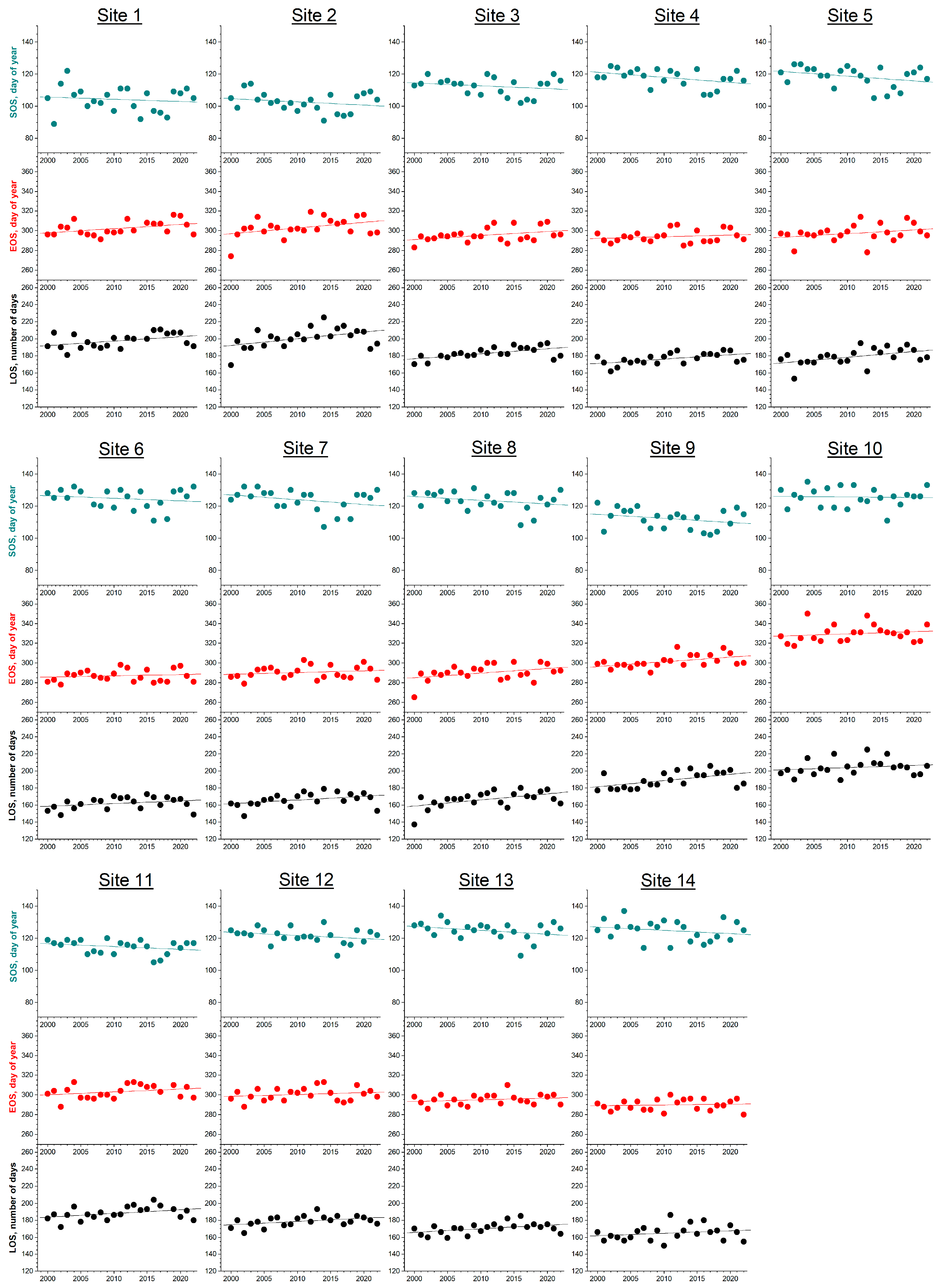
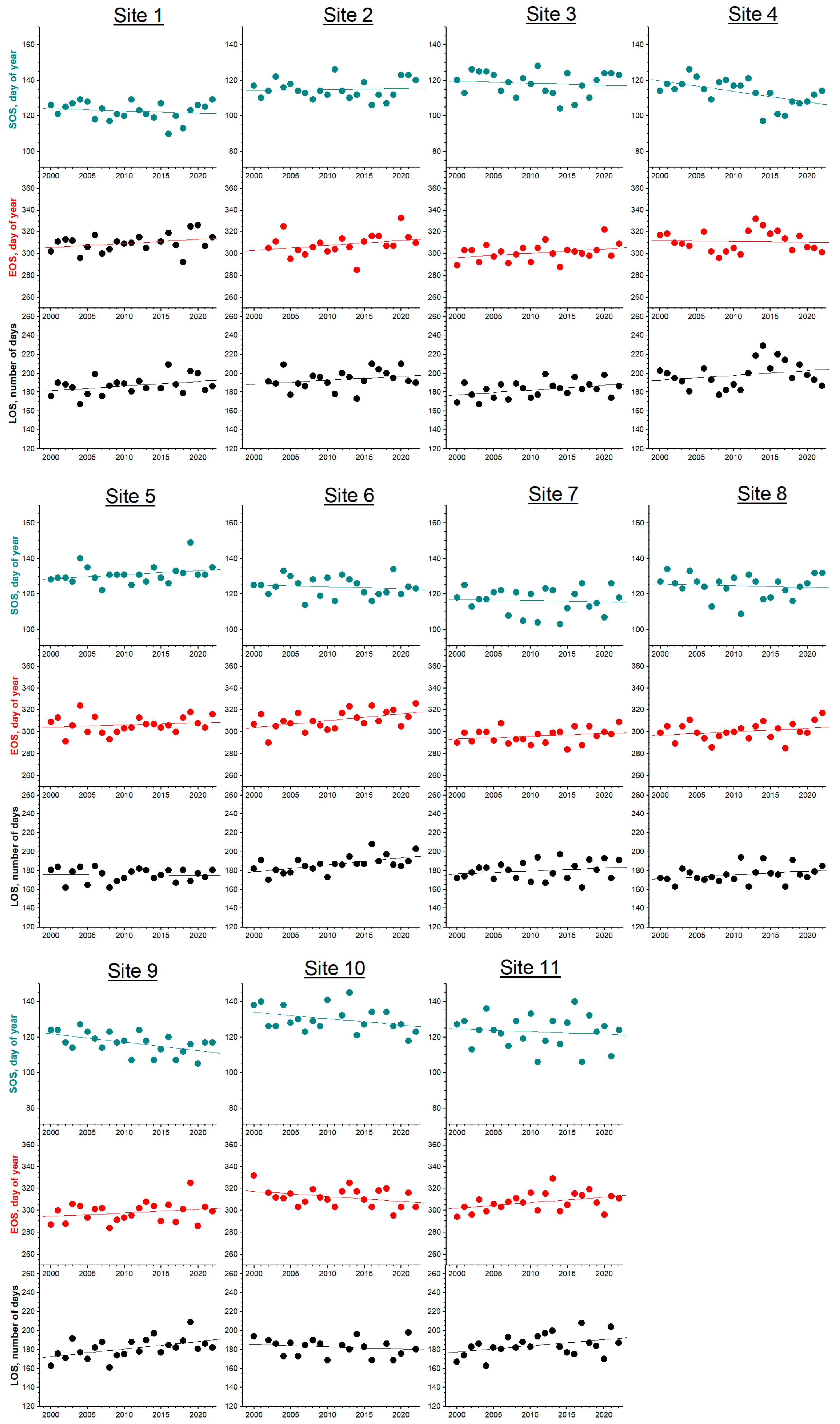
3.1. Phenology
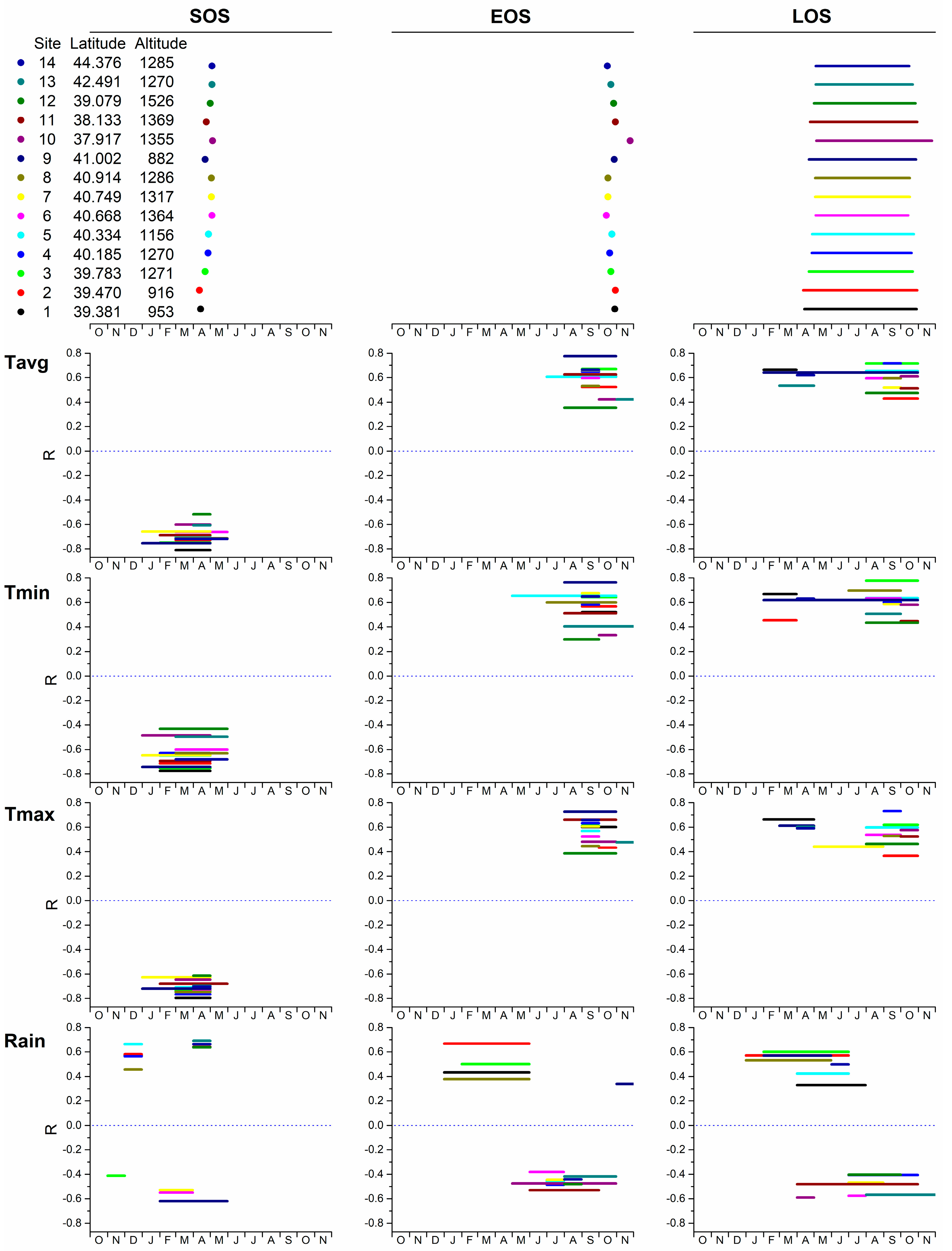
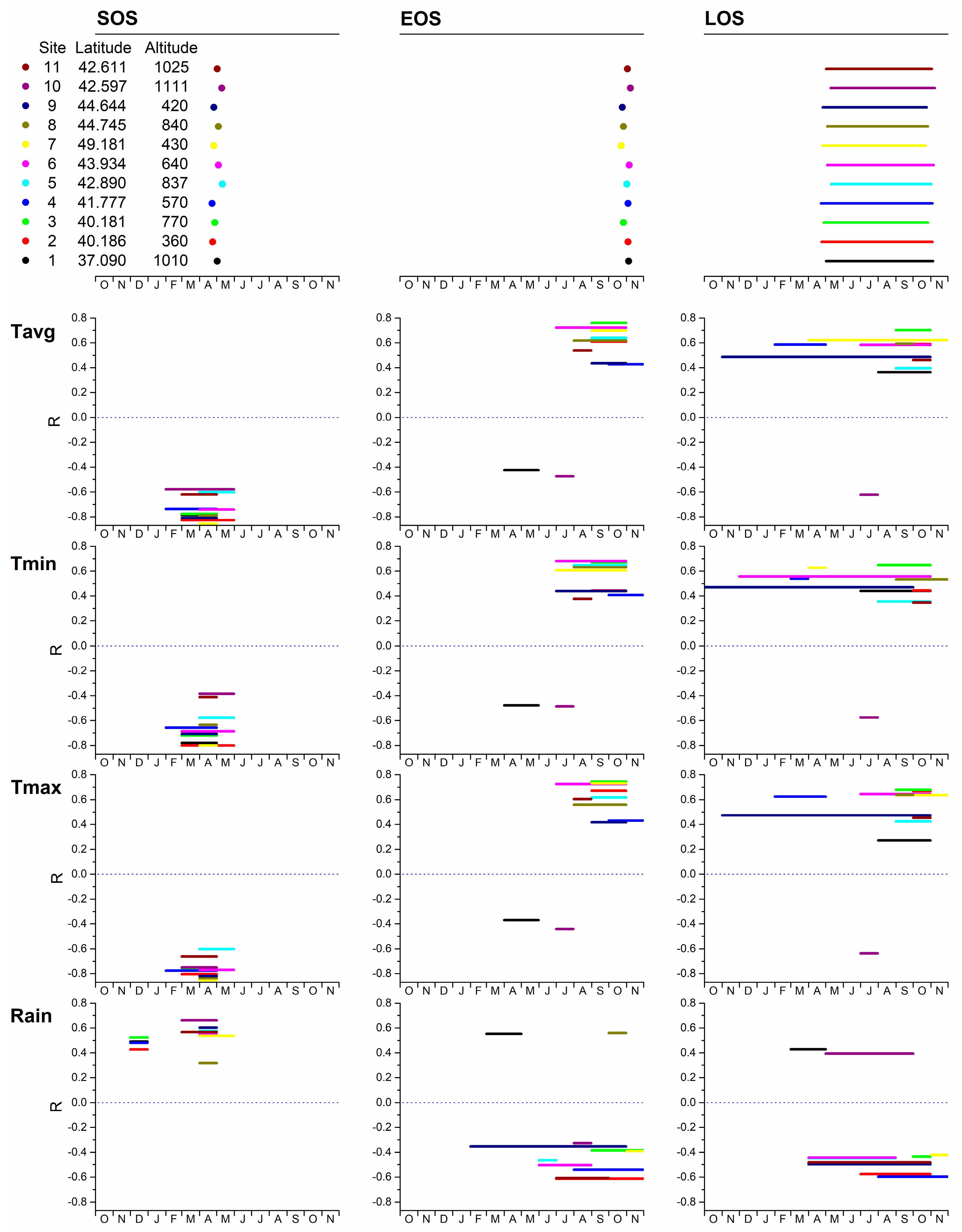
3.2. Phenology and Climate
4. Discussion
4.1. Phenology
4.2. Climate Effects
5. Conclusions
Author Contributions
Funding
Data Availability Statement
Acknowledgments
Conflicts of Interest
References
- Phenology and Seasonality Modeling; Lieth, H., Ed.; Ecological Studies; Springer: Berlin/Heidelberg, Germany, 1974; Volume 8, ISBN 978-3-642-51865-2. [Google Scholar]
- Piao, S.; Liu, Q.; Chen, A.; Janssens, I.A.; Fu, Y.; Dai, J.; Liu, L.; Lian, X.; Shen, M.; Zhu, X. Plant Phenology and Global Climate Change: Current Progresses and Challenges. Glob. Change Biol. 2019, 25, 1922–1940. [Google Scholar] [CrossRef]
- Berra, E.F.; Gaulton, R. Remote Sensing of Temperate and Boreal Forest Phenology: A Review of Progress, Challenges and Opportunities in the Intercomparison of in-Situ and Satellite Phenological Metrics. For. Ecol. Manag. 2021, 480, 118663. [Google Scholar] [CrossRef]
- Bajocco, S.; Raparelli, E.; Teofili, T.; Bascietto, M.; Ricotta, C. Text Mining in Remotely Sensed Phenology Studies: A Review on Research Development, Main Topics, and Emerging Issues. Remote Sens. 2019, 11, 2751. [Google Scholar] [CrossRef]
- Vitasse, Y.; Porté, A.J.; Kremer, A.; Michalet, R.; Delzon, S. Responses of Canopy Duration to Temperature Changes in Four Temperate Tree Species: Relative Contributions of Spring and Autumn Leaf Phenology. Oecologia 2009, 161, 187–198. [Google Scholar] [CrossRef] [PubMed]
- Fu, Y.H.; Zhao, H.; Piao, S.; Peaucelle, M.; Peng, S.; Zhou, G.; Ciais, P.; Huang, M.; Menzel, A.; Peñuelas, J.; et al. Declining Global Warming Effects on the Phenology of Spring Leaf Unfolding. Nature 2015, 526, 104–107. [Google Scholar] [CrossRef]
- Pretzsch, H.; Biber, P.; Schütze, G.; Uhl, E.; Rötzer, T. Forest Stand Growth Dynamics in Central Europe Have Accelerated since 1870. Nat. Commun. 2014, 5, 4967. [Google Scholar] [CrossRef]
- Gill, A.L.; Gallinat, A.S.; Sanders-DeMott, R.; Rigden, A.J.; Short Gianotti, D.J.; Mantooth, J.A.; Templer, P.H. Changes in Autumn Senescence in Northern Hemisphere Deciduous Trees: A Meta-Analysis of Autumn Phenology Studies. Ann. Bot. 2015, 116, 875–888. [Google Scholar] [CrossRef]
- Peñuelas, J.; Rutishauser, T.; Filella, I. Phenology Feedbacks on Climate Change. Science 2009, 324, 887–888. [Google Scholar] [CrossRef]
- Richardson, A.D.; Keenan, T.F.; Migliavacca, M.; Ryu, Y.; Sonnentag, O.; Toomey, M. Climate Change, Phenology, and Phenological Control of Vegetation Feedbacks to the Climate System. Agric. For. Meteorol. 2013, 169, 156–173. [Google Scholar] [CrossRef]
- Chuine, I.; Cour, P. Climatic Determinants of Budburst Seasonality in Four Temperate-Zone Tree Species. New Phytol. 1999, 143, 339–349. [Google Scholar] [CrossRef]
- Vitasse, Y.; François, C.; Delpierre, N.; Dufrêne, E.; Kremer, A.; Chuine, I.; Delzon, S. Assessing the Effects of Climate Change on the Phenology of European Temperate Trees. Agric. For. Meteorol. 2011, 151, 969–980. [Google Scholar] [CrossRef]
- IPCC. Climate Change 2023: Synthesis Report. Contribution of Working Groups I, II and III to the Sixth Assessment Report of IPCC; IPCC: Geneve, Switzerland, 2023. [Google Scholar]
- Gu, H.; Qiao, Y.; Xi, Z.; Rossi, S.; Smith, N.G.; Liu, J.; Chen, L. Warming-Induced Increase in Carbon Uptake Is Linked to Earlier Spring Phenology in Temperate and Boreal Forests. Nat. Commun. 2022, 13, 3698. [Google Scholar] [CrossRef]
- Haverd, V.; Smith, B.; Canadell, J.G.; Cuntz, M.; Mikaloff-Fletcher, S.; Farquhar, G.; Woodgate, W.; Briggs, P.R.; Trudinger, C.M. Higher than Expected CO2 Fertilization Inferred from Leaf to Global Observations. Glob. Change Biol. 2020, 26, 2390–2402. [Google Scholar] [CrossRef]
- Kharouba, H.M.; Ehrlén, J.; Gelman, A.; Bolmgren, K.; Allen, J.M.; Travers, S.E.; Wolkovich, E.M. Global Shifts in the Phenological Synchrony of Species Interactions over Recent Decades. Proc. Natl. Acad. Sci. USA 2018, 115, 5211–5216. [Google Scholar] [CrossRef] [PubMed]
- Fitter, A.H.; Fitter, R.S.R.; Harris, I.T.B.; Williamson, M.H. Relationships Between First Flowering Date and Temperature in the Flora of a Locality in Central England. Funct. Ecol. 1995, 9, 55. [Google Scholar] [CrossRef]
- Gonsamo, A.; Chen, J.M.; Wu, C. Citizen Science: Linking the Recent Rapid Advances of Plant Flowering in Canada with Climate Variability. Sci. Rep. 2013, 3, 2239. [Google Scholar] [CrossRef]
- Liang, L.; Schwartz, M.D.; Fei, S. Validating Satellite Phenology through Intensive Ground Observation and Landscape Scaling in a Mixed Seasonal Forest. Remote Sens. Environ. 2011, 115, 143–157. [Google Scholar] [CrossRef]
- Morellato, L.P.C.; Alberton, B.; Alvarado, S.T.; Borges, B.; Buisson, E.; Camargo, M.G.G.; Cancian, L.F.; Carstensen, D.W.; Escobar, D.F.E.; Leite, P.T.P.; et al. Linking Plant Phenology to Conservation Biology. Biol. Conserv. 2016, 195, 60–72. [Google Scholar] [CrossRef]
- Polgar, C.A.; Primack, R.B. Leaf out Phenology in Temperate Forests. Biodivers. Sci. 2013, 21, 111–116. [Google Scholar] [CrossRef]
- Zeng, L.; Wardlow, B.D.; Xiang, D.; Hu, S.; Li, D. A Review of Vegetation Phenological Metrics Extraction Using Time-Series, Multispectral Satellite Data. Remote Sens. Environ. 2020, 237, 111511. [Google Scholar] [CrossRef]
- De Beurs, K.M.; Henebry, G.M. Land Surface Phenology and Temperature Variation in the International Geosphere–Biosphere Program High-latitude Transects. Glob. Change Biol. 2005, 11, 779–790. [Google Scholar] [CrossRef]
- Friedl, M.; Henebry, G.; Reed, B.; Huete, A.; White, M.; Morisette, J.; Nemani, R.; Zhang, X.; Myneni, R. Land Surface Phenology. In NASA Whitepapers; NASA: Washington, DC, USA, 2006. [Google Scholar]
- Şenel, T.; Kanmaz, O.; Bektas Balcik, F.; Avcı, M.; Dalfes, H.N. Assessing Phenological Shifts of Deciduous Forests in Turkey under Climate Change: An Assessment for Fagus Orientalis with Daily MODIS Data for 19 Years. Forests 2023, 14, 413. [Google Scholar] [CrossRef]
- Uphus, L.; Lüpke, M.; Yuan, Y.; Benjamin, C.; Englmeier, J.; Fricke, U.; Ganuza, C.; Schwindl, M.; Uhler, J.; Menzel, A. Climate Effects on Vertical Forest Phenology of Fagus Sylvatica l., Sensed by Sentinel-2, Time Lapse Camera, and Visual Ground Observations. Remote Sens. 2021, 13, 3982. [Google Scholar] [CrossRef]
- Lukasová, V.; Bucha, T.; Škvareninová, J.; Škvarenina, J. Validation and Application of European Beech Phenological Metrics Derived from MODIS Data along an Altitudinal Gradient. Forests 2019, 10, 60. [Google Scholar] [CrossRef]
- Helman, D. Land Surface Phenology: What Do We Really ‘See’ from Space? Sci. Total Environ. 2018, 618, 665–673. [Google Scholar] [CrossRef]
- Rouse, R.W.H.; Haas, J.A.W.; Deering, D.W. Monitoring Vegetation Systems in the Great Plains with Erts. In Proceedings of the Goddard Space Flight Center 3rd ERTS-1 Symposium, Washington, DC, USA, 10–14 December 1973; pp. 309–317. [Google Scholar]
- Huete, A.; Didan, K.; Miura, T.; Rodriguez, X.; Gao, X.; Ferreira, L. Overview of the Radiometric and Biophysical Performance of the MODIS Vegetation Indices. Remote Sens. Environ. 2002, 83, 195–213. [Google Scholar] [CrossRef]
- Delbart, N.; Beaubien, E.; Kergoat, L.; Le Toan, T. Comparing Land Surface Phenology with Leafing and Flowering Observations from the PlantWatch Citizen Network. Remote Sens. Environ. 2015, 160, 273–280. [Google Scholar] [CrossRef]
- Schwartz, M.D.; Reed, B.C.; White, M.A. Assessing Satellite-derived Start-of-season Measures in the Conterminous USA. Int. J. Climatol. 2002, 22, 1793–1805. [Google Scholar] [CrossRef]
- Klosterman, S.; Melaas, E.; Wang, J.; Martinez, A.; Frederick, S.; O’Keefe, J.; Orwig, D.A.; Wang, Z.; Sun, Q.; Schaaf, C.; et al. Fine-Scale Perspectives on Landscape Phenology from Unmanned Aerial Vehicle (UAV) Photography. Agric. For. Meteorol. 2018, 248, 397–407. [Google Scholar] [CrossRef]
- Fisher, J.I.; Mustard, J.F.; Vadeboncoeur, M.A. Green Leaf Phenology at Landsat Resolution: Scaling from the Field to the Satellite. Remote Sens. Environ. 2006, 100, 265–279. [Google Scholar] [CrossRef]
- Alberton, B.; da Silva Torres, R.; Sanna Freire Silva, T.; Rocha, H.; S. B. Moura, M.; Morellato, L. Leafing Patterns and Drivers across Seasonally Dry Tropical Communities. Remote Sens. 2019, 11, 2267. [Google Scholar] [CrossRef]
- Belda, S.; Pipia, L.; Morcillo-Pallarés, P.; Rivera-Caicedo, J.P.; Amin, E.; De Grave, C.; Verrelst, J. DATimeS: A Machine Learning Time Series GUI Toolbox for Gap-Filling and Vegetation Phenology Trends Detection. Environ. Model. Softw. 2020, 127, 104666. [Google Scholar] [CrossRef]
- Jeong, S.J.; Ho, C.H.; Gim, H.J.; Brown, M.E. Phenology Shifts at Start vs. End of Growing Season in Temperate Vegetation over the Northern Hemisphere for the Period 1982–2008. Glob. Change Biol. 2011, 17, 2385–2399. [Google Scholar] [CrossRef]
- Wang, X.; Piao, S.; Xu, X.; Ciais, P.; Macbean, N.; Myneni, R.B.; Li, L. Has the Advancing Onset of Spring Vegetation Green-up Slowed down or Changed Abruptly over the Last Three Decades? Glob. Ecol. Biogeogr. 2015, 24, 621–631. [Google Scholar] [CrossRef]
- Garonna, I.; De Jong, R.; Stöckli, R.; Schmid, B.; Schenkel, D.; Schimel, D.; Schaepman, M.E. Shifting Relative Importance of Climatic Constraints on Land Surface Phenology. Environ. Res. Lett. 2018, 13, aaa17b. [Google Scholar] [CrossRef]
- Ibáñez, I.; Primack, R.B.; Miller-Rushing, A.J.; Ellwood, E.; Higuchi, H.; Lee, S.D.; Kobori, H.; Silander, J.A. Forecasting Phenology under Global Warming. Philos. Trans. R. Soc. B Biol. Sci. 2010, 365, 3247–3260. [Google Scholar] [CrossRef]
- Martinez del Castillo, E.; Zang, C.S.; Buras, A.; Hacket-Pain, A.; Esper, J.; Serrano-Notivoli, R.; Hartl, C.; Weigel, R.; Klesse, S.; Resco de Dios, V.; et al. Climate-Change-Driven Growth Decline of European Beech Forests. Commun. Biol. 2022, 5, 163. [Google Scholar] [CrossRef]
- Guo, L.; Dai, J.; Ranjitkar, S.; Xu, J.; Luedeling, E. Response of Chestnut Phenology in China to Climate Variation and Change. Agric. For. Meteorol. 2013, 180, 164–172. [Google Scholar] [CrossRef]
- Forzieri, G.; Girardello, M.; Ceccherini, G.; Spinoni, J.; Feyen, L.; Hartmann, H.; Beck, P.S.A.; Camps-Valls, G.; Chirici, G.; Mauri, A.; et al. Emergent Vulnerability to Climate-Driven Disturbances in European Forests. Nat. Commun. 2021, 12, 1081. [Google Scholar] [CrossRef]
- White, M.A.; Nemani, R.R. Real-Time Monitoring and Short-Term Forecasting of Land Surface Phenology. Remote Sens. Environ. 2006, 104, 43–49. [Google Scholar] [CrossRef]
- Abatzoglou, J.T.; Dobrowski, S.Z.; Parks, S.A.; Hegewisch, K.C. TerraClimate, a High-Resolution Global Dataset of Monthly Climate and Climatic Water Balance from 1958–2015. Sci. Data 2018, 5, 1–12. [Google Scholar] [CrossRef]
- Panchen, Z.A.; Primack, R.B.; Gallinat, A.S.; Nordt, B.; Stevens, A.D.; Du, Y.; Fahey, R. Substantial Variation in Leaf Senescence Times among 1360 Temperate Woody Plant Species: Implications for Phenology and Ecosystem Processes. Ann. Bot. 2015, 116, 865–873. [Google Scholar] [CrossRef]
- Čufar, K.; de Luis, M.; Saz, M.A.; Črepinšek, Z.; Kajfež-Bogataj, L. Temporal Shifts in Leaf Phenology of Beech (Fagus Sylvatica) Depend on Elevation. Trees—Struct. Funct. 2012, 26, 1091–1100. [Google Scholar] [CrossRef]
- Hwang, T.; Song, C.; Vose, J.M.; Band, L.E. Topography-Mediated Controls on Local Vegetation Phenology Estimated from MODIS Vegetation Index. Landsc. Ecol. 2011, 26, 541–556. [Google Scholar] [CrossRef]
- Dragoni, D.; Rahman, A.F. Trends in Fall Phenology across the Deciduous Forests of the Eastern USA. Agric. For. Meteorol. 2012, 157, 96–105. [Google Scholar] [CrossRef]
- Vitasse, Y.; Hoch, G.; Randin, C.F.; Lenz, A.; Kollas, C.; Scheepens, J.F.; Körner, C. Elevational Adaptation and Plasticity in Seedling Phenology of Temperate Deciduous Tree Species. Oecologia 2013, 171, 663–678. [Google Scholar] [CrossRef]
- Xia, H.; Qin, Y.; Feng, G.; Meng, Q.; Cui, Y.; Song, H.; Ouyang, Y.; Liu, G. Forest Phenology Dynamics to Climate Change and Topography in a Geographic and Climate Transition Zone: The Qinling Mountains in Central China. Forests 2019, 10, 1007. [Google Scholar] [CrossRef]
- Jiang, S.; Chen, X.; Huang, R.; Wang, T.; Smettem, K. Effect of the Altitudinal Climate Change on Growing Season Length for Deciduous Broadleaved Forest in Southwest China. Sci. Total Environ. 2022, 828, 154306. [Google Scholar] [CrossRef]
- Han, Q.; Luo, G.; Li, C. Remote Sensing-Based Quantification of Spatial Variation in Canopy Phenology of Four Dominant Tree Species in Europe. J. Appl. Remote Sens. 2013, 7, 073485. [Google Scholar] [CrossRef]
- Zhao, J.; Zhang, H.; Zhang, Z.; Guo, X.; Li, X.; Chen, C. Spatial and Temporal Changes in Vegetation Phenology at Middle and High Latitudes of the Northern Hemisphere over the Past Three Decades. Remote Sens. 2015, 7, 10973–10995. [Google Scholar] [CrossRef]
- Schwartz, M.D. Monitoring Global Change with Phenology: The Case of the Spring Green Wave. Int. J. Biometeorol. 1994, 38, 18–22. [Google Scholar] [CrossRef]
- Schwartz, M.D.; Ahas, R.; Aasa, A. Onset of Spring Starting Earlier across the Northern Hemisphere. Glob. Change Biol. 2006, 12, 343–351. [Google Scholar] [CrossRef]
- Fitchett, J.M.; Grab, S.W.; Thompson, D.I. Plant Phenology and Climate Change: Progress in Methodological Approaches and Application. Prog. Phys. Geogr. 2015, 39, 460–482. [Google Scholar] [CrossRef]
- Gonsamo, A.; Chen, J.M. Circumpolar Vegetation Dynamics Product for Global Change Study. Remote Sens. Environ. 2016, 182, 13–26. [Google Scholar] [CrossRef]
- Menzel, A.; Fabian, P. Growing Season Extended in Europe. Nature 1999, 397, 659. [Google Scholar] [CrossRef]
- Skvareninova, J.; Sitko, R.; Vido, J.; Snopková, Z.; Skvarenina, J. Phenological Response of European Beech (Fagus sylvatica L.) to Climate Change in the Western Carpathian Climatic-Geographical Zones. Front. Plant Sci. 2024, 15, 1242695. [Google Scholar] [CrossRef]
- Piao, S.; Tan, J.; Chen, A.; Fu, Y.H.; Ciais, P.; Liu, Q.; Janssens, I.A.; Vicca, S.; Zeng, Z.; Jeong, S.J.; et al. Leaf Onset in the Northern Hemisphere Triggered by Daytime Temperature. Nat. Commun. 2015, 6, 6911. [Google Scholar] [CrossRef]
- Liu, Q.; Fu, Y.H.; Zeng, Z.; Huang, M.; Li, X.; Piao, S. Temperature, Precipitation, and Insolation Effects on Autumn Vegetation Phenology in Temperate China. Glob. Change Biol. 2016, 22, 644–655. [Google Scholar] [CrossRef]
- Ge, Q.; Wang, H.; Rutishauser, T.; Dai, J. Phenological Response to Climate Change in China: A Meta-Analysis. Glob. Change Biol. 2015, 21, 265–274. [Google Scholar] [CrossRef]
- Myneni, R.B.; Keeling, C.D.; Tucker, C.J.; Asrar, G.; Nemani, R.R. Increased Plant Growth in the Northern High Latitudes from 1981 to 1991. Nature 1997, 386, 698–702. [Google Scholar] [CrossRef]
- Guo, J.; Hu, Y. Spatiotemporal Variations in Satellite-Derived Vegetation Phenological Parameters in Northeast China. Remote Sens. 2022, 14, 705. [Google Scholar] [CrossRef]
- Garonna, I.; de Jong, R.; Schaepman, M.E. Variability and Evolution of Global Land Surface Phenology over the Past Three Decades (1982–2012). Glob. Change Biol. 2016, 22, 1456–1468. [Google Scholar] [CrossRef]
- Vitasse, Y.; Signarbieux, C.; Fu, Y.H. Global Warming Leads to More Uniform Spring Phenology across Elevations. Proc. Natl. Acad. Sci. USA 2018, 115, 1004–1008. [Google Scholar] [CrossRef] [PubMed]
- Jaworski, T.; Hilszczański, J. The Effect of Temperature and Humidity Changes on Insects Development Their Impact on Forest Ecosystems in the Expected Climate Change. For. Res. Pap. 2013, 74, 345–355. [Google Scholar] [CrossRef]
- Chuine, I. Why Does Phenology Drive Species Distribution? Philos. Trans. R. Soc. B Biol. Sci. 2010, 365, 3149–3160. [Google Scholar] [CrossRef] [PubMed]
- Peñuelas, J.; Filella, I. Phenology—Responses to a Warming World. Science 2001, 294, 793–795. [Google Scholar] [CrossRef]
- Grossiord, C.; Bachofen, C.; Gisler, J.; Mas, E.; Vitasse, Y.; Didion-Gency, M. Warming May Extend Tree Growing Seasons and Compensate for Reduced Carbon Uptake during Dry Periods. J. Ecol. 2022, 110, 1575–1589. [Google Scholar] [CrossRef]
- Gordo, O.; Sanz, J.J. Impact of Climate Change on Plant Phenology in Mediterranean Ecosystems. Glob. Change Biol. 2010, 16, 1082–1106. [Google Scholar] [CrossRef]
- Xu, L.; Chen, X.Q. Spatial Modeling of the Ulmus Pumila Growing Season in China’s Temperate Zone. Sci. China Earth Sci. 2012, 55, 656–664. [Google Scholar] [CrossRef]
- Chen, X.; Luo, X.; Xu, L. Comparison of Spatial Patterns of Satellite-Derived and Ground-Based Phenology for the Deciduous Broadleaf Forest of China. Remote Sens. Lett. 2013, 4, 532–541. [Google Scholar] [CrossRef]
- Chmielewski, F.M.; Rotzer, T. Response of Tree Phenology to Climate Change across Europe. Agric. For. Meteorol. 2001, 108, 101–112. [Google Scholar] [CrossRef]
- Buermann, W.; Bikash, P.R.; Jung, M.; Burn, D.H.; Reichstein, M. Earlier Springs Decrease Peak Summer Productivity in North American Boreal Forests. Environ. Res. Lett. 2013, 8, 024027. [Google Scholar] [CrossRef]
- Fu, Y.H.; Piao, S.; Zhao, H.; Jeong, S.J.; Wang, X.; Vitasse, Y.; Ciais, P.; Janssens, I.A. Unexpected Role of Winter Precipitation in Determining Heat Requirement for Spring Vegetation Green-up at Northern Middle and High Latitudes. Glob. Change Biol. 2014, 20, 3743–3755. [Google Scholar] [CrossRef]
- Keenan, T.F.; Richardson, A.D. The Timing of Autumn Senescence Is Affected by the Timing of Spring Phenology: Implications for Predictive Models. Glob. Change Biol. 2015, 21, 2634–2641. [Google Scholar] [CrossRef]
- Xian, Z.; Yu, Z.; Agathokleous, E.; Han, W.; You, W.; Zhou, G. Trends and Climate-Sensitivity of Phenology in China’s Natural and Planted Forests. J. Geophys. Res. Biogeosci. 2024, 129, e2023JG007955. [Google Scholar] [CrossRef]
- Xie, Y.; Wang, X.; Silander, J.A. Deciduous Forest Responses to Temperature, Precipitation, and Drought Imply Complex Climate Change Impacts. Proc. Natl. Acad. Sci. USA 2015, 112, 13585–13590. [Google Scholar] [CrossRef]
- Fu, Y.H.; Piao, S.; Op de Beeck, M.; Cong, N.; Zhao, H.; Zhang, Y.; Menzel, A.; Janssens, I.A. Recent Spring Phenology Shifts in Western Central Europe Based on Multiscale Observations. Glob. Ecol. Biogeogr. 2014, 23, 1255–1263. [Google Scholar] [CrossRef]


| Species | Site | Longitude, ° | Latitude, ° | Elevation, m a.s.l. | Annual Tavg, °C | Annual Precipitation, mm |
|---|---|---|---|---|---|---|
| Fagus sylvatica | 1 | 23.139 | 39.381 | 953 | 14.1 ± 0.3 | 589 ± 118 |
| 2 | 23.041 | 39.470 | 916 | 12.2 ± 0.3 | 642 ± 127 | |
| 3 | 22.747 | 39.783 | 1271 | 10.3 ± 0.4 | 688 ± 148 | |
| 4 | 22.167 | 40.185 | 1270 | 9.8 ± 0.4 | 648 ± 125 | |
| 5 | 22.229 | 40.334 | 1156 | 12.1 ± 0.4 | 527 ± 104 | |
| 6 | 21.399 | 40.668 | 1364 | 9.1 ± 0.5 | 790 ± 144 | |
| 7 | 21.328 | 40.749 | 1317 | 8.3 ± 0.5 | 837 ± 151 | |
| 8 | 21.876 | 40.914 | 1286 | 8.3 ± 0.5 | 701 ± 131 | |
| 9 | 21.934 | 41.002 | 882 | 9.3 ± 0.4 | 641 ± 119 | |
| 10 | 14.864 | 37.917 | 1355 | 10.8 ± 0.3 | 677 ± 120 | |
| 11 | 15.836 | 38.133 | 1369 | 9.3 ± 0.3 | 805 ± 139 | |
| 12 | 16.673 | 39.079 | 1526 | 9.9 ± 0.3 | 881 ± 145 | |
| 13 | 13.415 | 42.491 | 1270 | 7.5 ± 0.4 | 798 ± 133 | |
| 14 | 10.097 | 44.376 | 1285 | 9.4 ± 0.5 | 1502 ± 289 | |
| Castanea sativa | 1 | 22.750 | 37.090 | 1010 | 13.6 ± 0.3 | 769 ± 135 |
| 2 | 24.345 | 40.186 | 360 | 14.6 ± 0.4 | 596 ± 107 | |
| 3 | 24.329 | 40.181 | 770 | 13.5 ± 0.4 | 623 ± 113 | |
| 4 | 12.725 | 41.777 | 570 | 13.8 ± 0.4 | 601 ± 108 | |
| 5 | 11.564 | 42.890 | 837 | 12.6 ± 0.5 | 575 ± 106 | |
| 6 | 10.670 | 43.934 | 640 | 13.9 ± 0.5 | 1197 ± 231 | |
| 7 | 7.996 | 49.181 | 430 | 10.2 ± 0.6 | 827 ± 114 | |
| 8 | 4.329 | 44.745 | 840 | 10.3 ± 0.6 | 920 ± 154 | |
| 9 | 2.379 | 44.644 | 420 | 12.2 ± 0.6 | 673 ± 82 | |
| 10 | −7.079 | 42.597 | 1111 | 9.4 ± 0.3 | 1369 ± 251 | |
| 11 | −7.119 | 42.611 | 1025 | 9.0 ± 0.3 | 1413 ± 259 |
| Site | Latitude, ° | Elevation, m | SOS, DOY | R | p | Slope, NOD Year−1 | EOS, DOY | R | p | Slope, NOD Year−1 | LOS, DOY | R | p | Slope, NOD Year−1 |
|---|---|---|---|---|---|---|---|---|---|---|---|---|---|---|
| 1 | 39.381 | 953 | 104 ± 8 | −0.118 | 0.590 | −0.137 | 302 ± 7 | 0.413 | 0.056 | 0.422 | 198 ± 8 | 0.429 | 0.047 | 0.523 |
| 2 | 39.470 | 916 | 103 ± 6 | −0.230 | 0.290 | −0.201 | 303 ± 10 | 0.398 | 0.060 | 0.577 | 201 ± 12 | 0.448 | 0.032 | 0.778 |
| 3 | 39.783 | 1271 | 112 ± 6 | −0.214 | 0.338 | −0.176 | 295 ± 7 | 0.398 | 0.060 | 0.413 | 183 ± 7 | 0.589 | 0.004 | 0.588 |
| 4 | 40.185 | 1270 | 118 ± 5 | −0.405 | 0.062 | −0.318 | 294 ± 6 | 0.187 | 0.392 | 0.169 | 177 ± 7 | 0.539 | 0.010 | 0.510 |
| 5 | 40.334 | 1156 | 118 ± 6 | −0.320 | 0.137 | −0.295 | 297 ± 9 | 0.289 | 0.181 | 0.373 | 179 ± 10 | 0.465 | 0.025 | 0.668 |
| 6 | 40.668 | 1364 | 125 ± 6 | −0.180 | 0.423 | −0.160 | 287 ± 6 | 0.144 | 0.513 | 0.125 | 162 ± 7 | 0.308 | 0.163 | 0.315 |
| 7 | 40.749 | 1317 | 124 ± 7 | −0.306 | 0.165 | −0.297 | 290 ± 6 | 0.188 | 0.389 | 0.176 | 166 ± 8 | 0.394 | 0.070 | 0.444 |
| 8 | 40.914 | 1286 | 123 ± 6 | −0.274 | 0.206 | −0.237 | 290 ± 8 | 0.393 | 0.064 | 0.473 | 167 ± 9 | 0.514 | 0.012 | 0.710 |
| 9 | 41.002 | 882 | 112 ± 6 | −0.274 | 0.205 | −0.247 | 302 ± 6 | 0.499 | 0.015 | 0.478 | 189 ± 9 | 0.523 | 0.010 | 0.725 |
| 10 | 37.917 | 1355 | 126 ± 6 | −0.046 | 0.835 | −0.041 | 330 ± 9 | 0.173 | 0.431 | 0.221 | 204 ± 9 | 0.192 | 0.380 | 0.262 |
| 11 | 38.133 | 1369 | 115 ± 4 | −0.278 | 0.198 | −0.174 | 303 ± 7 | 0.287 | 0.195 | 0.288 | 188 ± 8 | 0.389 | 0.074 | 0.435 |
| 12 | 39.079 | 1526 | 122 ± 5 | −0.283 | 0.191 | −0.195 | 301 ± 7 | 0.194 | 0.374 | 0.188 | 179 ± 6 | 0.427 | 0.042 | 0.382 |
| 13 | 42.491 | 1270 | 125 ± 5 | −0.310 | 0.149 | −0.243 | 295 ± 5 | 0.212 | 0.331 | 0.169 | 170 ± 6 | 0.437 | 0.037 | 0.412 |
| 14 | 44.376 | 1285 | 125 ± 6 | −0.221 | 0.310 | −0.206 | 290 ± 5 | 0.102 | 0.645 | 0.081 | 165 ± 9 | 0.221 | 0.311 | 0.287 |
| All sites | 118 ± 8 | −0.209 ± 0.073 | 299 ± 11 | 0.297 ± 0.157 | 181 ± 14 | 0.503 ± 0.170 | ||||||||
| Site | Latitude, ° | Elevation, m | SOS, DOY | R | p | Slope, NOD Year−1 | EOS, DOY | R | p | Slope, NOD Year−1 | LOS, DOY | R | p | Slope, NOD Year−1 |
|---|---|---|---|---|---|---|---|---|---|---|---|---|---|---|
| 1 | 37.090 | 1010 | 123 ± 5 | −0.171 | 0.437 | −0.127 | 310 ± 8 | 0.309 | 0.161 | 0.372 | 187 ± 10 | 0.352 | 0.108 | 0.489 |
| 2 | 40.186 | 360 | 115 ± 5 | 0.065 | 0.767 | 0.051 | 309 ± 10 | 0.284 | 0.213 | 0.460 | 194 ± 10 | 0.262 | 0.251 | 0.430 |
| 3 | 40.181 | 770 | 118 ± 7 | −0.114 | 0.604 | −0.113 | 301 ± 8 | 0.343 | 0.109 | 0.398 | 183 ± 9 | 0.393 | 0.064 | 0.511 |
| 4 | 41.777 | 570 | 113 ± 7 | −0.552 | 0.006 | −0.592 | 308 ± 17 | 0.135 | 0.541 | 0.331 | 195 ± 21 | 0.303 | 0.161 | 0.923 |
| 5 | 42.890 | 837 | 131 ± 5 | 0.294 | 0.173 | 0.237 | 307 ± 8 | 0.175 | 0.425 | 0.203 | 175 ± 7 | −0.033 | 0.881 | −0.035 |
| 6 | 43.934 | 640 | 124 ± 5 | −0.128 | 0.561 | −0.103 | 311 ± 9 | 0.497 | 0.016 | 0.633 | 187 ± 9 | 0.573 | 0.004 | 0.736 |
| 7 | 49.181 | 430 | 116 ± 7 | −0.065 | 0.767 | −0.068 | 296 ± 7 | 0.256 | 0.239 | 0.256 | 180 ± 10 | 0.226 | 0.300 | 0.324 |
| 8 | 44.745 | 840 | 125 ± 6 | −0.094 | 0.670 | −0.090 | 301 ± 8 | 0.271 | 0.212 | 0.321 | 176 ± 9 | 0.321 | 0.136 | 0.411 |
| 9 | 44.644 | 420 | 117 ± 6 | −0.521 | 0.011 | −0.473 | 298 ± 9 | 0.235 | 0.281 | 0.322 | 181 ± 11 | 0.502 | 0.015 | 0.795 |
| 10 | 42.597 | 1111 | 130 ± 7 | −0.352 | 0.118 | −0.360 | 312 ± 9 | −0.355 | 0.105 | −0.460 | 183 ± 9 | −0.177 | 0.455 | −0.233 |
| 11 | 42.611 | 1025 | 123 ± 9 | −0.112 | 0.612 | −0.150 | 308 ± 8 | 0.400 | 0.058 | 0.500 | 185 ± 11 | 0.392 | 0.064 | 0.650 |
| All sites | 121 ± 6 | −0.163 ± 0.234 | 306 ± 6 | 0.303 ± 0.28 | 184 ± 6 | 0.455 ± 0.345 |
| Fagus | Castanea | |||||||||||
|---|---|---|---|---|---|---|---|---|---|---|---|---|
| Variable | t | p | VIF | Variable Change | Phenology Change | Variable | t | p | VIF | Variable Change | Phenology Change | |
| SOS | Tmax_APR | −6.572 | <0.001 | 1.836 | 1 °C | −1.103 days | Tmax_APR | −11.114 | <0.001 | 2.588 | 1 °C | −3.309 days |
| Elevation | 8.994 | <0.001 | 1.664 | Tmin_APR | 4.972 | <0.001 | 2.696 | 1 °C | 1.431 days | |||
| Tmin_FEB | −4.887 | <0.001 | 1.215 | 1 °C | −0.816 days | Rain_MAR | 3.733 | <0.001 | 1.143 | |||
| Latitude | 4.522 | <0.001 | 1.18 | |||||||||
| EOS | Tmin_SEP | 12.169 | <0.001 | 1.500 | 1 °C | 3.133 days | Latitude | −2.427 | 0.016 | 1.483 | ||
| Latitude | −11.898 | <0.001 | 1.376 | Rain_APR | 4.8 | <0.001 | 1.365 | |||||
| Tmax_MAY | −9.905 | <0.001 | 1.996 | 1 °C | −2.15 days | Tmin_OCT | 6.536 | <0.001 | 2.534 | 1 °C | 2.220 days | |
| Elevation | −7.482 | <0.001 | 1.767 | Tmin_MAY | −6.01 | <0.001 | 2.794 | 1 °C | −1.859 days | |||
| Tmax_FEB | −3.522 | <0.001 | 1.634 | 1 °C | −0.765 days | Tmax_SEP | 3.982 | <0.001 | 2.152 | 1 °C | 1.366 days | |
| LOS | Tmin_SEP | 13.299 | <0.001 | 1.329 | 1 °C | 3.326 days | Tmax_OCT | 3.648 | <0.001 | 2.005 | 1 °C | 1.597 days |
| Latitude | −15.522 | <0.001 | 1.365 | Tmax_SEP | 3.679 | <0.001 | 2.287 | 1 °C | 1.637 days | |||
| Elevation | −15.11 | <0.001 | 1.746 | Tmin_MAY | −3.822 | <0.001 | 2.073 | 1 °C | −1.286 days | |||
| Tmax_MAY | −9.309 | <0.001 | 1.858 | 1 °C | −2.010 days | Tmax_FEB | 2.23 | 0.027 | 1.146 | 1 °C | 0.698 days | |
| Tmax_APR | 1.973 | 0.05 | 1.79 | 1 °C | 0.766 days |
Disclaimer/Publisher’s Note: The statements, opinions and data contained in all publications are solely those of the individual author(s) and contributor(s) and not of MDPI and/or the editor(s). MDPI and/or the editor(s) disclaim responsibility for any injury to people or property resulting from any ideas, methods, instructions or products referred to in the content. |
© 2025 by the authors. Licensee MDPI, Basel, Switzerland. This article is an open access article distributed under the terms and conditions of the Creative Commons Attribution (CC BY) license (https://creativecommons.org/licenses/by/4.0/).
Share and Cite
Doumkou, O.; Markaki, M.; Vanikiotis, T.; Kyparissis, A. Climate Effects on Phenology of Two Deciduous Forest Species Across Southern Europe. Forests 2025, 16, 608. https://doi.org/10.3390/f16040608
Doumkou O, Markaki M, Vanikiotis T, Kyparissis A. Climate Effects on Phenology of Two Deciduous Forest Species Across Southern Europe. Forests. 2025; 16(4):608. https://doi.org/10.3390/f16040608
Chicago/Turabian StyleDoumkou, Olga, Maria Markaki, Theofilos Vanikiotis, and Aris Kyparissis. 2025. "Climate Effects on Phenology of Two Deciduous Forest Species Across Southern Europe" Forests 16, no. 4: 608. https://doi.org/10.3390/f16040608
APA StyleDoumkou, O., Markaki, M., Vanikiotis, T., & Kyparissis, A. (2025). Climate Effects on Phenology of Two Deciduous Forest Species Across Southern Europe. Forests, 16(4), 608. https://doi.org/10.3390/f16040608