Article

Algorithm for Detecting Trees Affected by Pine Wilt Disease in Complex Scenes Based on CNN-Transformer

1
College of Information Engineering, Northwest A&F University, Yangling 712100, China
2
Intelligent Equipment Research Center, Beijing Academy of Agriculture and Forestry Sciences, Beijing 100097, China
*
Authors to whom correspondence should be addressed.
Forests 2025, 16(4), 596; https://doi.org/10.3390/f16040596
Submission received: 17 February 2025 / Revised: 19 March 2025 / Accepted: 26 March 2025 / Published: 28 March 2025
(This article belongs to the Section Forest Inventory, Modeling and Remote Sensing)

Abstract

:
Pine wilt disease, a highly destructive forest disease with rapid spread, currently has no effective treatments. Infected pine trees usually die within a few months, causing severe damage to forest ecosystems. A rapid and accurate detection algorithm for diseased trees is crucial for curbing the spread of this disease. In recent years, the combination of drone remote sensing and deep learning has become the main methods of detecting and locating diseased trees. Previous studies have shown that increasing network depth cannot improve accuracy in this task. Therefore, a lightweight semantic segmentation model based on a CNN-Transformer hybrid architecture was designed in this study, named EVitNet. This segmentation model reduces network parameters while improving recognition accuracy, outperforming mainstream models. The segmentation IoU for discolored trees reached 0.713, with only 1.195 M parameters. Furthermore, considering the diverse and complex terrain where diseased trees are distributed, a fine-tuning model approach was adopted. After a small amount of training, the IoU on new samples increased from 0.321 to 0.735, greatly enhancing the practicality of the algorithm. The model’s segmentation speed in the task of discolored trees identification meets the requirements of real-time performance, and its accuracy exceeds that of mainstream semantic segmentation models. In the future, it is expected to be deployed on drones for real-time recognition, accelerating the entire process of discovering and locating infected trees.

1. Introduction

Currently, nearly 10 pine tree diseases are prevalent, among which pine wilt disease (PWD), caused by the pine wood nematode (PWN), is the major one and is highly contagious and extremely destructive [1]. It was first discovered in North America [2] and is now prevalent in countries such as China, Japan, South Korea, the United States, Canada, Portugal, and Mexico. This disease has caused widespread death of pine trees in multiple countries, resulting in significant ecological damage [3]. In Japan, the first case of PWD was discovered in the early twentieth century, and by 2019, the disease had spread in all prefectures except Hokkaido. In China, the first infected pine tree was found in Nanjing in 1982, with a spread rate of 7000~10,000 hectares per year [4], and by 2023, the disease had spread to 19 provinces (encompassing 701 counties and cities) [5]. When the PWN invades pine trees, it first destroys the xylem tissue cells, hindering water transport and causing the needles to gradually turn reddish-brown [6]. Once infected, pine trees usually die within a few months [7]. Since there are no effective treatment measures for this disease, the most effective control measure is to locate and fell the infected trees for clearance [8]. A more pressing issue is that the PWN is now spreading to areas with previously unsuitable climates, moving northward and to higher altitudes [9]. To effectively prevent the further spread of pine wilt disease and avoid greater ecological damage, there is an urgent need to accelerate the process of locating infected trees for felling and crushing, with the goal of harmless treatment [10].
Artificial intelligence (AI) has shown transformative potential across multiple fields. For instance, Koy et al. [11] shows AI optimizing high-frequency trading strategies; Purohit et al. [12] highlights deep learning’s significance in medical image segmentation; and Chiphiko et al. [13] underscores AI’s role in enhancing IoT security protocols. These examples show AI’s broad applicability. Similarly, in pest and disease identification, AI significantly boosts efficiency [14,15]. Traditional monitoring of pine wilt disease mainly relies on manual surveys, which are time-consuming and labor-intensive. Moreover, most pine trees are located in areas with steep mountains and dense forests, making it difficult for survey personnel to reach [16]. Monitoring using drone and satellite remote sensing technologies can greatly improve efficiency. However, satellite remote sensing is still limited by its low spatial resolution and long revisit cycle, resulting in low accuracy and long monitoring intervals [17]. Drone remote sensing has the advantages of high flexibility, high spatial resolution, and low cost. Using drone remote sensing technology to monitor PWD-affected discolored trees (hereinafter referred to as “discolored trees”) has become the main method for detecting and locating discolored trees [18]. There have been many studies using object detection methods to identify discolored pine trees [19], but object detection methods often struggle with detection in scenes with overlap [20] and small targets [21]. In comparison, semantic segmentation is more suitable for remote sensing classification and recognition tasks. Remote sensing images are usually much larger than natural images, and semantic segmentation has a natural advantage in processing large-sized images. Additionally, semantic segmentation networks can extract delicate texture features of discolored trees at the pixel level, obtaining precise segmentation boundaries, which facilitates rapid estimation of the affected area.
Semantic segmentation was initially transformed to classification tasks through a sliding window approach, but this method was computationally redundant and inefficient. The advent of Fully Convolutional Networks (FCNs) [22] established the indelible status of encoder–decoder architecture-based networks in the domain of semantic segmentation. In the subsequent years, a plethora of segmentation networks grounded in the encoder–decoder structure emerged. For instance, UNet [23], which achieved state-of-the-art (SOTA) performance in the medical field when it was proposed, is a classic U-shaped symmetric network of the encoder–decoder architecture. It is typically suitable for datasets with low contrast, imbalance, and requirements for preserving fine details, such as medical datasets. In the general domain, Google introduced the prominent Deeplab series, which have now evolved to Deeplabv3+ [24]. Its excellent performance stems from the larger receptive field obtained through atrous convolution and the feature maps of different atrous rates fused via ASPP (Atrous Spatial Pyramid Pooling). In recent years, with the research on Transformers [25], technologies such as large models and multimodality have been better implemented. In the field of semantic segmentation, Meta introduced SAM [26]. This algorithm performs interactive segmentation and can “segment anything” without the need for retraining. As deep learning continues to evolve, current research trends are increasingly focused on combining a Transformer with a CNN to fully leverage the unique advantages of both.
Current research on semantic segmentation for discolored tree recognition mainly falls into two categories. One applies a single segmentation algorithm for identification, while the other evaluates the performance of multiple algorithms. There is a lack of specialized segmentation algorithms designed specifically for discolored tree recognition. As a result, mainstream segmentation algorithms often fall short in terms of accuracy and speed, and their robustness in complex environments leaves much to be desired. There is a notable absence of segmentation models specifically tailored for this task. In this study, we employed a lightweight Vision Transformer (ViT) as the encoder to capture the global features of discolored trees, thereby enhancing the network’s feature extraction capabilities. A Convolutional Neural Network (CNN) was utilized as the decoder, leveraging its inherent spatial inductive bias to ensure the precision of the decoding process. On the other hand, previous studies have overlooked the significant challenges to model generalizability posed by varying terrains, diverse tree species, and different sampling equipment. This task typically demands a high level of model generalizability. The optimal fine-tuning strategy will enable the model to maintain high accuracy with minimal new sample learning, thus enhancing its practicality. The main aims of this study are as follows:
(1)
To construct two high-quality semantic segmentation datasets from distinct terrain areas using different sampling equipment.
(2)
To develop an efficient and accurate discolored tree segmentation model (EVitNet) through the innovative integration of a lightweight ViT feature extraction network and a CNN upsampling method.
(3)
To identify the optimal fine-tuning strategy that improves the model’s practicality, allowing it to achieve high accuracy with only a small amount of new sample learning.

2. Materials and Methods

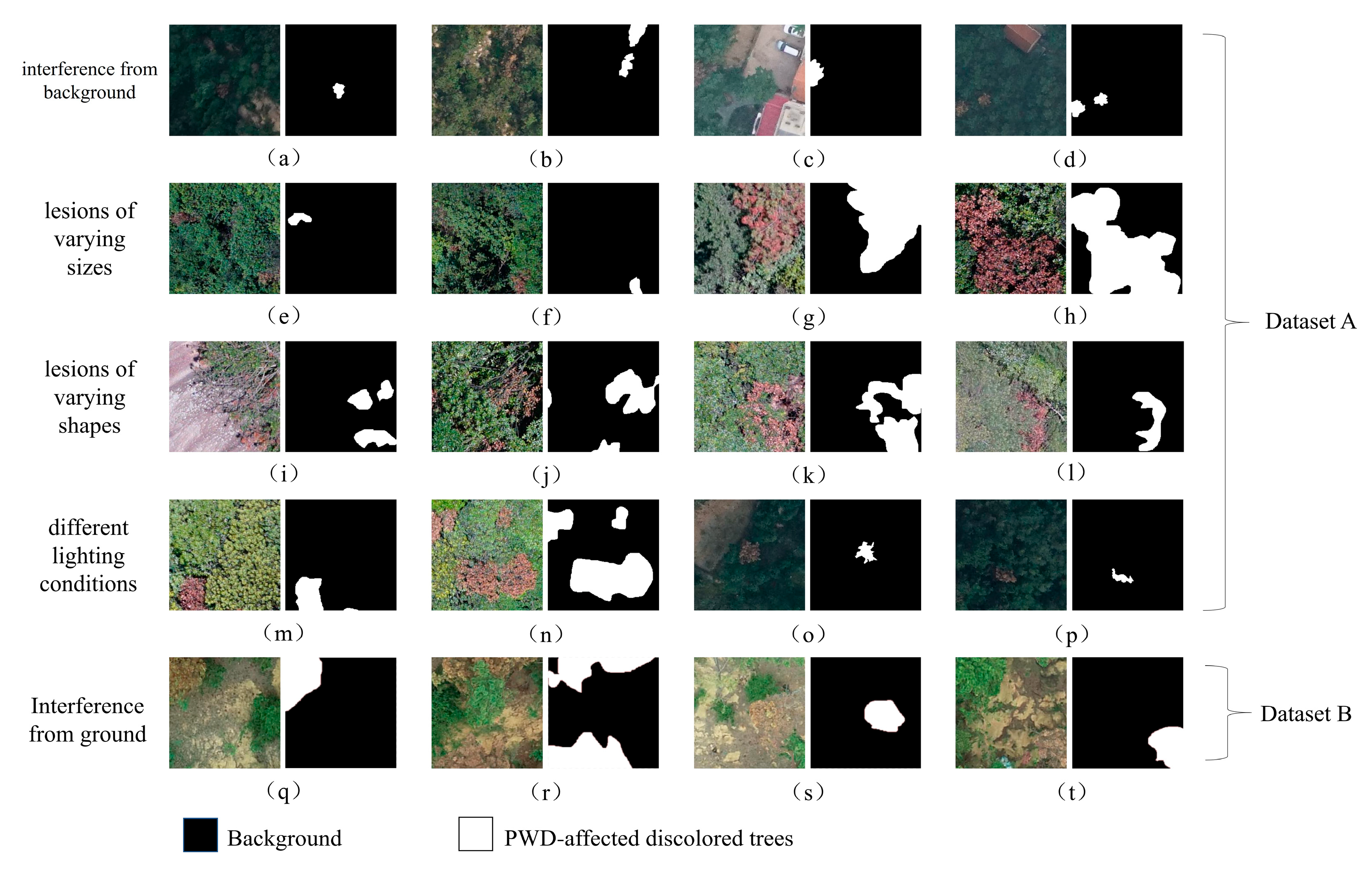
2.1. Data Collection
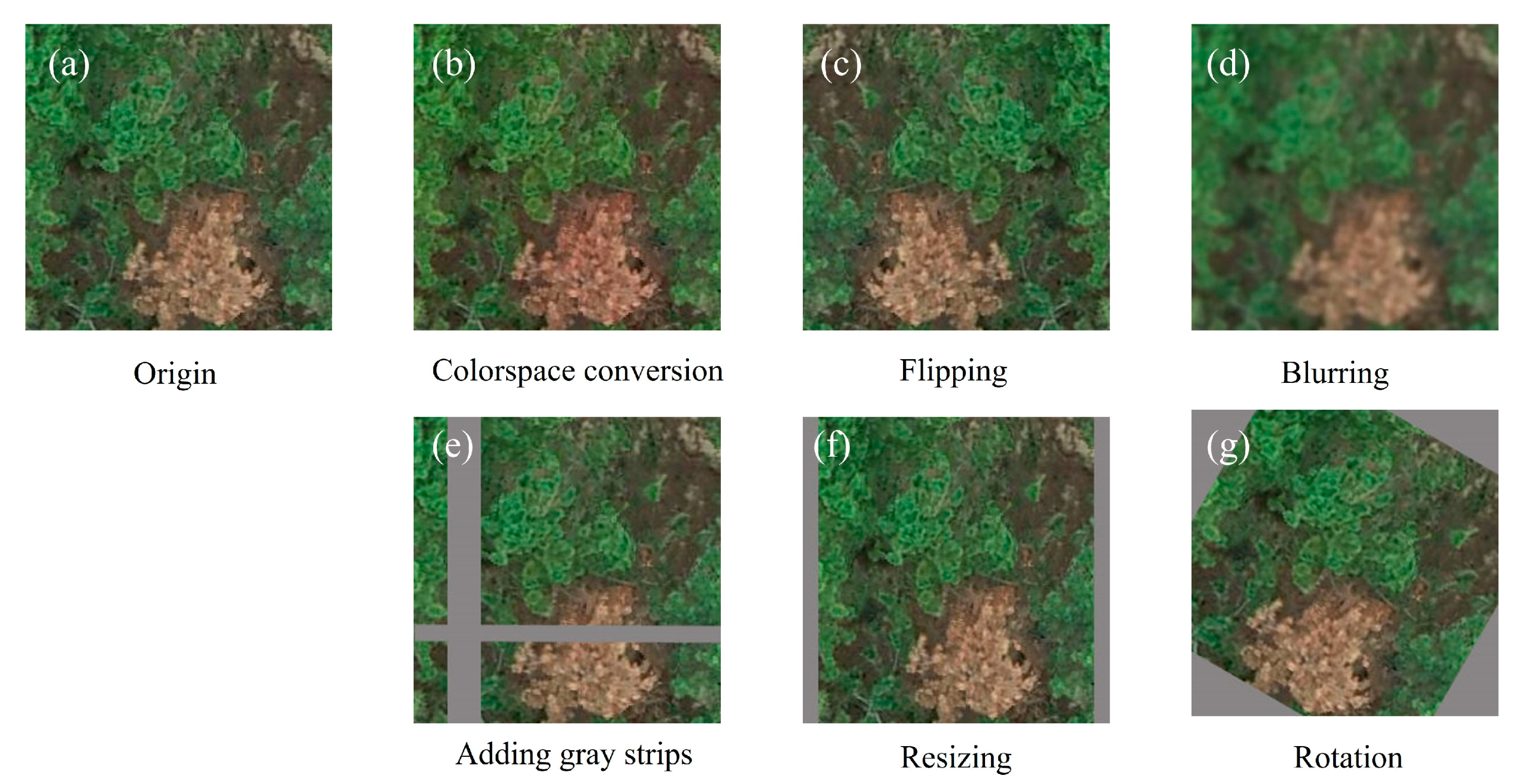
Two datasets of PWD-affected discolored trees were utilized in this study, with different sampling equipment being used in the two sampling areas (Figure 1). Dataset A was collected in Qingdao, Shandong (36°04′0.98″ N, 120°22′57.59″ E), using a DB-II fixed-wing drone equipped with a Sony Alpha 7R II camera, while Dataset B was collected in Yantai, Shandong (37°28′25.71″ N, 121°11′51.14″ E), using a DJI Phantom 4 Pro. The sampling area in Qingdao, Shandong, is mountainous terrain with an average elevation of 360 m and a maximum elevation of 1132.7 m. The main pine species are Pinus densiflora [27], and the photographed area covers 200 km². The sampling area in Yantai, Shandong, is flat coastal terrain with an average elevation of 9 m. The area of this sampling site is 0.7 km², and the main pine species are Pinus densiflora and Pinus thunbergii [28]. During sampling in both areas, images were captured at equal distances, with a flight direction overlap of no less than 75% and a lateral overlap of no less than 75%. Ultimately, more than 17,000 raw images with a resolution of 7952 × 5304 were obtained in Qingdao, Shandong, and a total of 1089 raw images with a resolution of 5472 × 3648 were obtained in Yantai, Shandong.
During sampling, equipment was selected based on the scene, with detailed dataset information (Table 1). In Qingdao, Shandong, given the large sampling area and high average elevation of discolored trees, a DB-II fixed-wing drone (Dabai Technology Co. Ltd.; China) equipped with a full-frame camera was used. Fixed-wing drones, with fast cruising speeds and long endurance, are suitable for large-scale data collection. They also have a high cruising altitude, fitting mountainous terrain. A high-pixel full-frame camera (Sony Alpha 7 R II, Sony Group Corporation, Japan) was used due to the high flight altitude. However, fixed-wing drones require a suitable runway for takeoff and landing. In contrast, quadcopters, though having lower sampling resolution, feature lower usage costs and fewer terrain restrictions, making them more appropriate for smaller scenes, such as those in Yantai, Shandong, so we chose the DJI Phantom 4 Pro (Da-Jiang Innovations Science and Technology Co., Ltd.; China) for sampling in Yantai.

2.2. Data Process

Raw aerial images contain a substantial amount of repetitive content. By utilizing Pix4DMapper software (version 4.5.6), the original aerial photographs were stitched together to create orthophotos (Figure 1), thereby achieving the goal of eliminating redundancy. Under the guidance of forest disease control experts, annotations were carried out based on the visual characteristics of discolored pine trees in remote sensing images. After pine trees are infected with PWN, their needles change from green to yellow or red, and resin secretion decreases [29]. These changes can be distinguished through spectral and texture feature analysis, which differentiates discolored trees from healthy pines and other similar-colored objects, enabling precise labeling. Subsequently, a script was employed to generate corresponding binary images based on the annotation information. Both the orthophotos and the binary images with annotation information were cropped to a size of 256 × 256. A total of 31,500 samples were obtained from the data collected in Qingdao, Shandong, with 2981 of them containing at least one discolored tree lesion. From the data gathered in Yantai, Shandong, 3753 samples were acquired, among which 524 had discolored tree lesions. Both datasets are characterized by extremely imbalanced sample distribution.
To facilitate the selection of samples containing discolored tree lesions, this study proposes an entirely new sample processing workflow, with the pseudocode presented in pseudocode 1. After processing with this code, samples containing lesions and their annotations can be stored in directory 1, while all samples can be stored in directory 2. This approach eliminates the need for manual screening of the dataset and also makes it easier to generate samples of different sizes in the future.
Pseudocode 1: Generate samples from xml annotation information
  • Open orthophoto to read image size and geographical transformation parameters
  • Create the whole annotated image
  • For annotations in xml file:
  •   Convert the UTM coordinate list to the pixel coordinate list
  •   Draw polygons according to pixel coordinates on the annotated image and fill them
  •   For blocks (256 × 256) in annotated image:
  •     If the block has annotation:
  •       Save the label and corresponding orthophoto block to Directory 1
  •     Save the label and corresponding orthophoto block to Directory 2
To facilitate subsequent experiments, samples containing lesions from the two sampling sites were used as two separate datasets, with each divided into a training set and a testing set at a 9:1 ratio. Some samples from the two datasets contain both typical discolored tree samples and various samples that may be difficult to identify (Figure 2). Dataset A includes situations such as similar color and texture of interfering objects and discolored trees, large-scale differences in discolored trees, various outlines, and different lighting conditions. In Dataset B, the sandy background poses strong interference to identification. Due to differences in terrain, tree species, and sampling equipment between the two sites, the two datasets differ significantly. The dataset from Qingdao, Shandong, is named Dataset A, and the dataset from Yantai, Shandong, is named Dataset B. Dataset A was used for model design and validation, while Dataset B was used to determine the fine-tuning learning strategy.
In the field of deep learning, the quality of data samples determines the final model performance and generalization ability. To ensure the model’s generalizability, data augmentation is commonly used to enhance the quality of data samples, generally by adding noise to the original images and performing random transformations [30]. Considering that the sample size is sufficient in this study, the efficient online augmentation method was adopted. During training, color space transformation and adjustment, random flipping, random blurring, random adding gray strips, random resizing, and random rotation were performed on the samples and labels to enhance the data, with the effects of augmentation (Figure 3).

2.3. Methods

2.3.1. The Semantic Segmentation Model for Discolored Trees, EVitNet

To enhance the accuracy and efficiency of discolored trees segmentation in complex scenes, this study constructed a lightweight discolored trees segmentation model, EVitNet (Easy Vision Transformer Net), based on Transformer and CNN as the basic network structures, featuring an encoder–decoder architecture. The algorithm is robust and capable of meeting the needs for precise and rapid segmentation of discolored trees in diverse scenarios. EVitNet combines the advantages of Transformer and CNN. The encoder section alternately employs CNN and Vision Transformer, enabling global feature encoding through Transformer while preserving spatial inductive bias via CNN. This effectively avoids the drawback of Transformer requiring massive data for training and reduces training costs [31]. The encoder with added Transformer blocks can better extract global features from the input, expanding the receptive field to the size of the entire image and enhancing the effectiveness of feature extraction. The decoder section draws on the upsampling structure of U-Net, imitating its skip connections to preserve shallow detail feature information, ensuring the precision of subsequent upsampling.
In the network structure diagram of EVitNet (Figure 4), for the input image, lightweight convolution based on depthwise separable convolution is employed. After the last three convolutional blocks, MobileVit Blocks are incorporated, enabling the network to perform global reorganization among sufficiently rich feature information. Before each downsampling, skip connections are used to retain all detail features. Each decoder in the network consists of a standard convolution and an expanded convolution. The expanded convolution enhances the upsampling accuracy without increasing the network parameters. After a series of upsampling operations, the final feature map is obtained, which is then mapped to two channels through a fully connected layer to complete the classification for each pixel.

2.3.2. EasyVit Backbone Network

In recent years, the Transformer architecture has revolutionized the fields of natural language processing and computer vision. In the realm of computer vision, ViT has achieved SOTA results in some tasks. However, ViT has a large number of parameters. Experiments have shown that using ViT with a large number of parameters does not lead to higher segmentation accuracy but significantly increases the computational burden. In this study, a lightweight ViT structure was adopted based on the design of MobileViT [32]. EasyViT was constructed using MobileViT Block and MobileNetv2 Block [33], and EasyViT was used as the feature extraction backbone network.
The MobileVit block commences with a standard convolutional layer, which is tasked with capturing the local feature information of the input tensor X. Subsequently, the feature information is projected into a higher-dimensional space through a convolutional operation, thereby enhancing the expressive power of the features and facilitating their subsequent flattening and input into the Transformer for global feature encoding. After obtaining the encoded results, they are restored to the original shape, and then the feature information is projected back to the input size through a convolutional operation and concatenated with the skip connection of the input X. Through a standard convolutional layer, the feature map with 2C channels is converted back to C channels, thus completing the global feature encoding in the spatial domain.
The MobileNetv2 block, a core component of MobileNetv2, shares a similar concept with the MobileViT block. Initially, project the feature information into a higher-dimensional space before further refining the features. For an input X, the MobileNetv2 block first expands the number of channels in the feature map through convolution. It then applies depthwise separable convolution and pointwise convolution separately. Replacing standard convolution with two separate convolutions reduces the number of parameters and computations. Finally, when the input and output feature maps have the same size, a residual connection is used to concatenate the two feature maps.

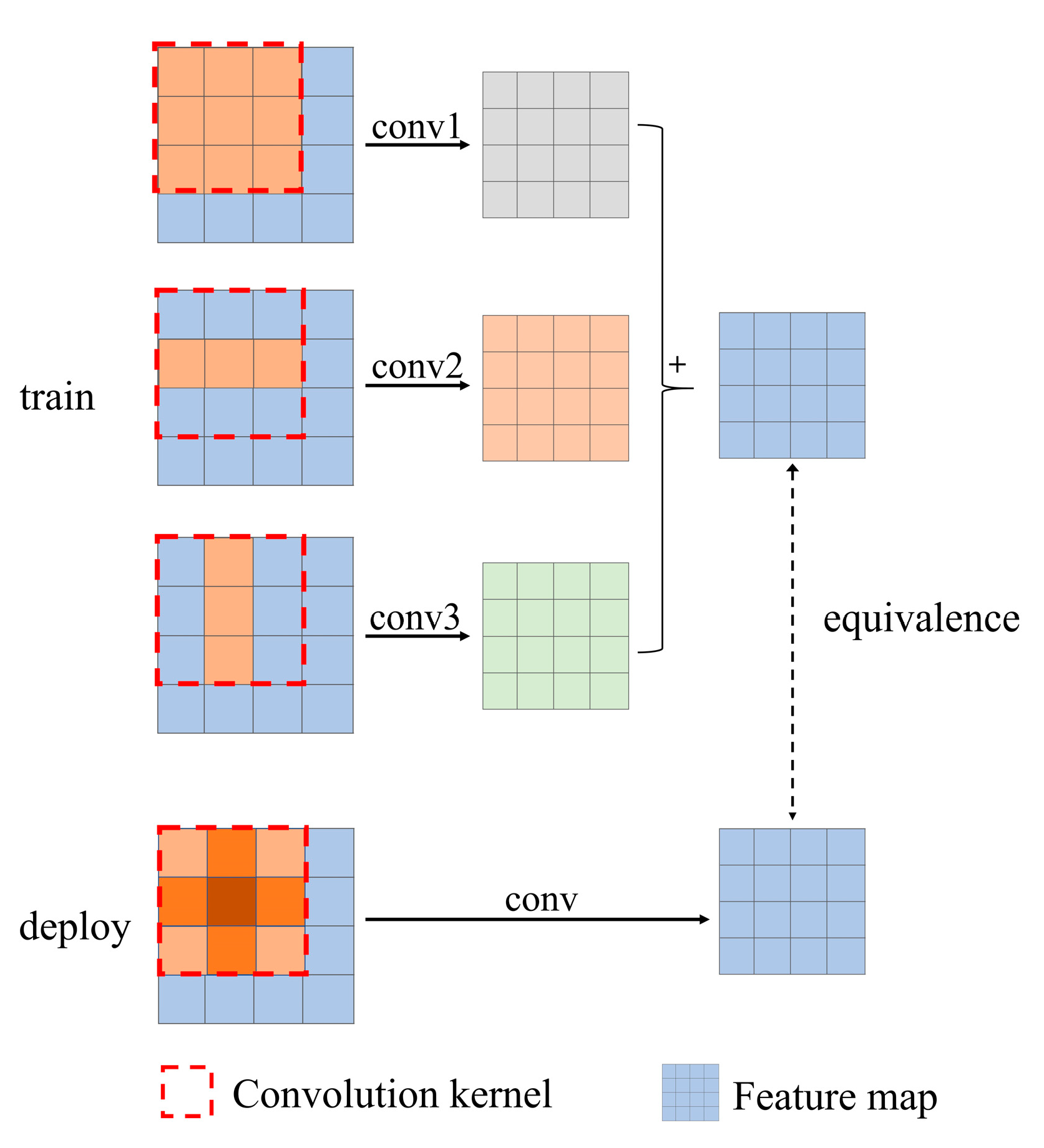
2.3.3. Decoder with Expanded Convolution

Controlling the number of network parameters is crucial for segmentation speed. Therefore, this study does not increase the parameters. Instead, it follows the design of MMDM [34] and replaces the traditional 3 × 3 standard convolutional blocks with three convolutions of 3 × 3, 1 × 3, and 3 × 1, effectively improving the accuracy of network upsampling. During training, the 9 parameters of the standard convolutional kernel expand to 15 parameters and then revert to 9 parameters during subsequent deployment, without increasing the number of parameters. This process is referred to as expanded convolution.
The expanded convolution block is illustrated (Figure 5). Since convolution has additivity, the outputs of several expanded convolutions are summed, which is equivalent to the outputs obtained by summing these convolution kernels. Therefore, expanded convolutions can be used to replace traditional convolutions. During training, the original convolution is decomposed into three convolutions, allowing for more parameters to refine the learning of feature processing methods. When deploying the model, the expanded convolution is merged into a standard convolution without adding extra parameters.

2.3.4. Model Fine-Tuning Method

After years of clearance and control, PWD is currently sporadic in multiple regions. The tree species affected by PWD are numerous and span many countries, making it difficult to achieve complete sampling coverage for the large number of tree species. Moreover, the economic viability of large-scale sampling and annotation is low. In response to this challenge, this study proposes fine-tuning the weights obtained through training, enabling the model to learn from a small amount of new data and maintain a high accuracy on the new dataset.
Fine-tuning the model is implemented through transfer learning, the main idea of which is to transfer labeled data or knowledge structures from related domains to enhance learning efficiency in the target domain. The premise of using transfer learning is that the source and target domains share some degree of similarity. The prior knowledge learned in the source domain is helpful for learning in the target domain. If the two domains are too different, using transfer learning may lead to negative transfer. In this study, both datasets are about PWD-affected discolored trees, which are highly similar and thus suitable for transfer learning. Dataset A, introduced in Section 2, is used as the base dataset because of its large scale, which allows for sufficient model training. Dataset B is used as the transfer learning validation dataset. The process of the two datasets and model fine-tuning is shown in Figure 6. The model is first trained conventionally on Dataset A. After training, based on the weights obtained from the previous training, a portion of samples from Dataset B is selected as incremental data for learning. A series of comparative experiments are designed to determine the optimal transfer learning strategy, focusing on whether to freeze the backbone network weights and what proportion of data to use for incremental learning.

2.4. Evaluation Metrics

In this study, four accuracy evaluation metrics were primarily used for the single category of discolored trees: IoU (Intersection over Union), F1 score, precision, and recall. Due to the presence of a large number of easily recognizable background negative samples in the samples, the mIoU (mean Intersection over Union) or mp (mean precision) would be artificially high, which is not conducive to comparing model performance. The identification accuracy of PWD-affected discolored trees by the model is the main focus, hence the primary use of single-category evaluation metrics for discolored trees. Initially used in object detection, IoU is employed to determine the difference between the predicted bounding box area and the true area, calculated by dividing the intersection area of the two regions by their union area. The value of IoU ranges from 0 to 1, with a value closer to 1 indicating a more accurate predicted box location. In semantic segmentation, the situation is similar, except that the shape of the detection and annotation areas changes from rectangles to irregular shapes. In a task with k categories, the calculation method for the IoU of the ith category is shown in Formula (1):
I o U = A r e a   o f   O v e r l a p A r e a   o f   U n i o n = p i i j = 0 k p i j + j = 0 k p j i p i i
In this context, p i j represents the number of pixels where the true label is class i and the predicted result is class j . When i = j , p i j indicates the number of correctly predicted pixels, and when i j , it indicates the number of incorrectly predicted pixels. Similarly, the calculation methods for precision and recall of class i are shown in Equation (2) and Equation (3), respectively.
P r e c i s i o n = T P T P + F P = p i i j = 0 k p j i
R e c a l l = T P T P + F N = p i i j = 0 k p i j
In this context, TP represents the number of correctly detected positive samples, while FP and FN denote the number of incorrectly detected positive samples and the number of incorrectly detected negative samples, respectively.
The F1 score is the harmonic mean of precision and recall, providing a more comprehensive representation of the model’s segmentation accuracy. The calculation method is presented in Formula (4):
F 1 s c o r e = 2 T P 2 T P + F P + F N
The model complexity is primarily determined by the number of parameters. The evaluation indicators for model complexity are the number of model parameters and the amount of inference computation. The unit for the number of parameters is M (minions), which represents the size of the total number of learnable parameters in the entire model. The unit for the amount of inference computation is GFLOPs (Giga floating point operations), which indicates the number of floating point operations required for model inference. The model segmentation speed is measured by FPS (frames per second), which represents the number of images the model can segment per second.

2.5. Experimental Setting

The experiments involved in this study were conducted on a Windows-based computing platform. The deep learning framework employed was PyTorch 1.13, with CUDA version 11.7, and the Python version was 3.8. The platform was equipped with a GeForce RTX 3090 GPU (NVIDIA Corporation, USA) and an Intel(R) Core (TM) i9–10940X CPU (Intel Corporation, USA) running at 3.30 GHz.

3. Results

3.1. The Problem of Unbalanced Positive and Negative Samples

The task of identifying PWD-affected discolored trees is quite unique. After epidemic prevention and clearance, the distribution of discolored trees is currently sparse. Most of the samples obtained through sampling contain only background and no target of discolored trees, which is a case of extreme sample imbalance. We tried using the focal loss function, which can greatly improve network performance. Considering that most of the information in the background has no positive impact on model training, we conducted experiments on the training set of Dataset A. Following the data processing method mentioned before, we selected samples containing discolored tree lesions for training and then validated them on the same validation set. The model accuracy obtained was higher than that of training on all original training sets, and it greatly saved training time.
Training with the filtered training set not only resulted in higher accuracy but also reduced the training time by 76.19% (Table 2). When there is a severe imbalance between positive and negative samples, focal loss can bring about substantial performance improvements. After data filtering, the sample imbalance issue was largely resolved, the precision of the background did not reduce, and the precision of the discolored tree rose. Based on these experimental results, the new sample processing workflow mentioned before was proposed.

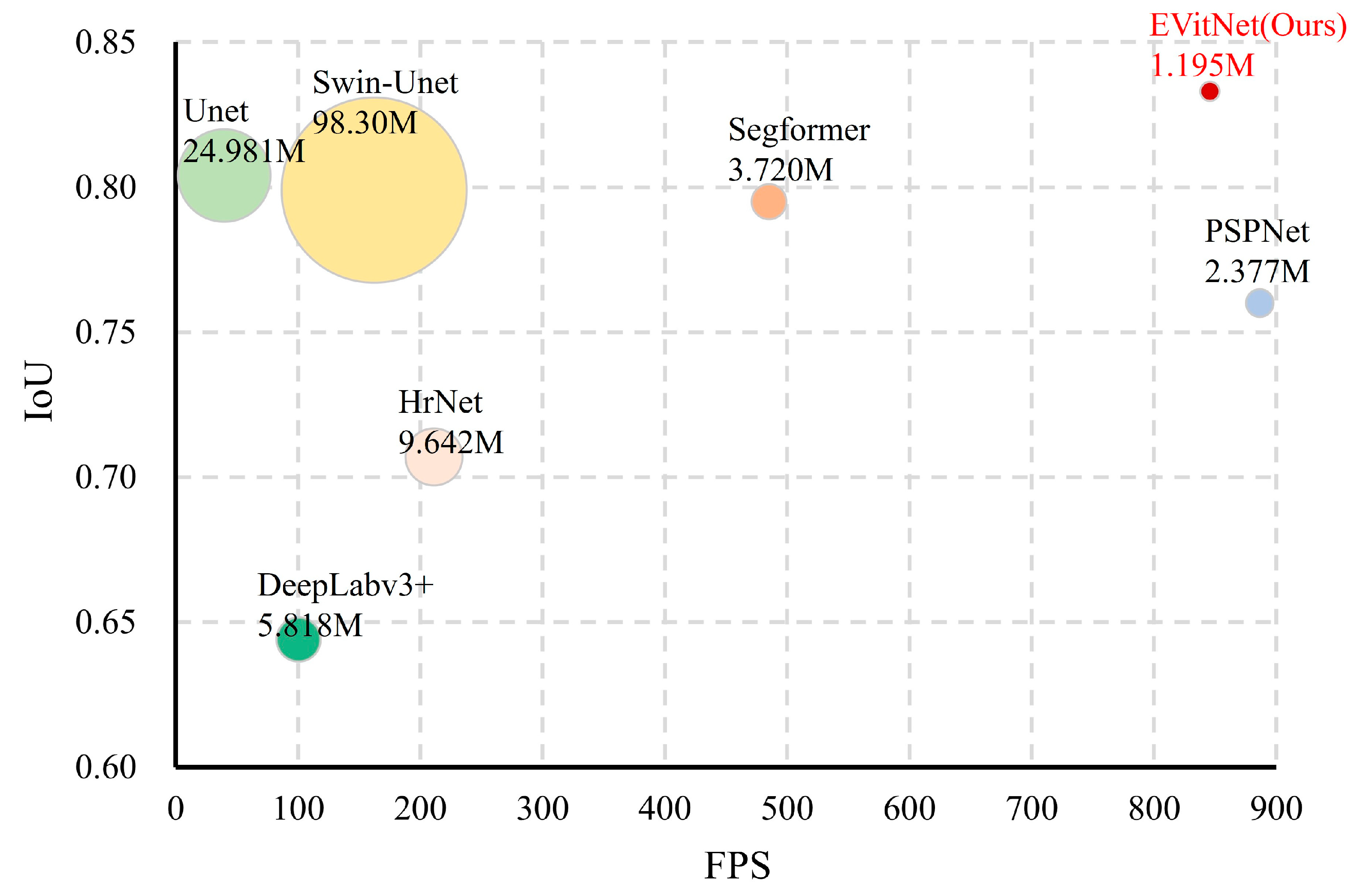
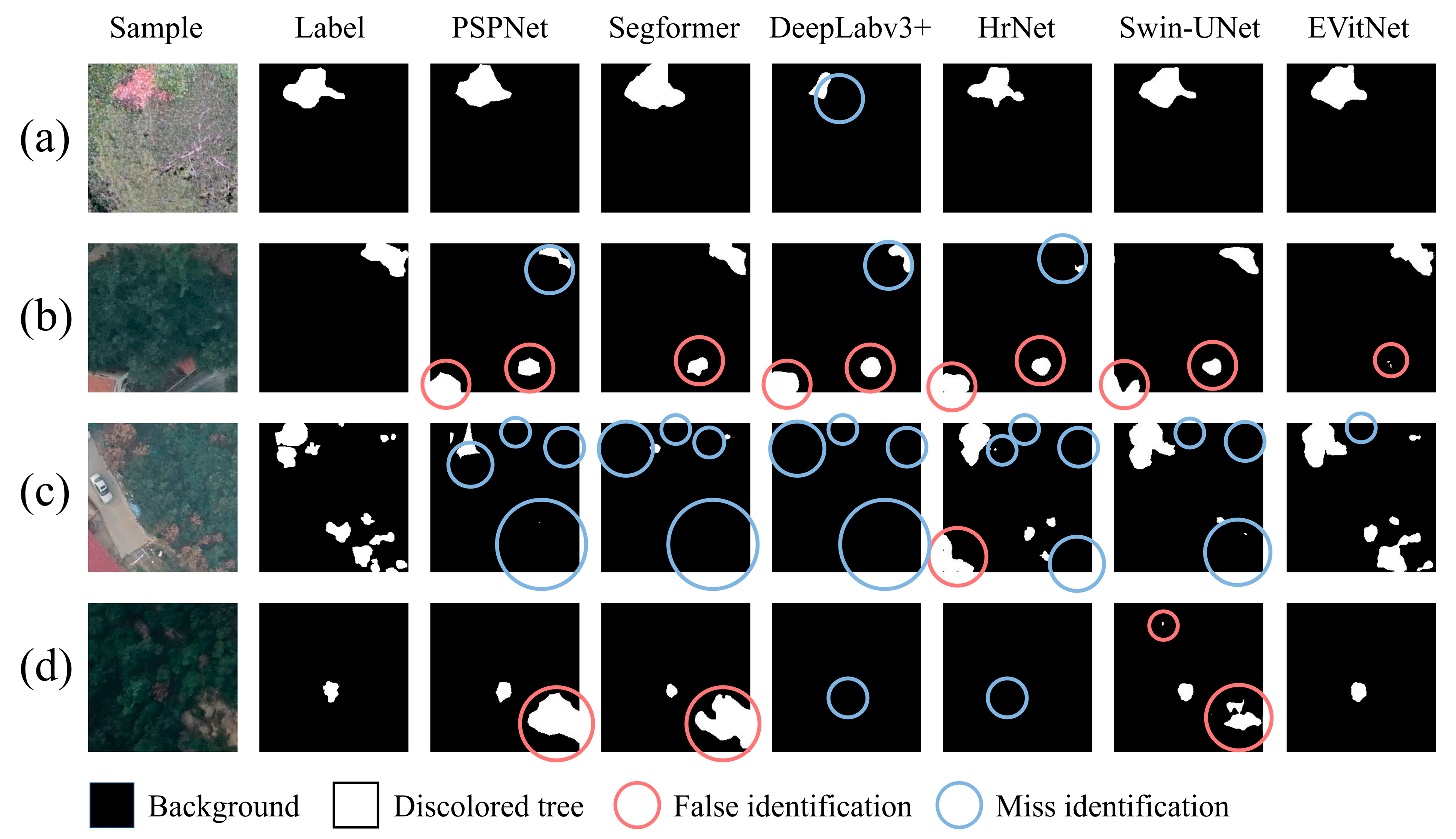
3.2. Comparison of Mainstream Models

A comparison was made between mainstream semantic segmentation models and the proposed EVitNet on the PWD-affected discolored tree Dataset A. The models included U-Net, DeepLabv3+, PSPNet [35], Segformer [36], HrNet [37], and Swin-UNet [38]. It is worth noting that SAM is an interactive model that requires inputting each target’s position for segmentation and is unable to perform automatic segmentation tasks. Therefore, it was not included in our comparison. The input size for all networks was standardized to 256 × 256. Additionally, all hyperparameters were kept consistent: batch size = 16, epochs = 100, and the Adam optimizer was used with a cosine annealing learning rate adjustment strategy. After training, the performance metrics mentioned before were calculated.
Based on the performance of each model on the discolored tree dataset, a scatter bubble chart was created (Figure 7). From the figure, it is evident that EVitNet exhibits significant advantages in terms of segmentation accuracy, parameter count, and speed.
The training loss and validation loss curves for each model are presented in Figure 8. The curves for the HrNet and DeepLabv3+ models exhibit a distinctive pattern, showing a noticeable secondary decline. This indicates that the complexity of the HrNet and DeepLabv3+ models is relatively high, which may not align well with the complexity of the discolored tree dataset, potentially leading them to become trapped in local optima during training. It illustrates that the implemented models have completed extensive training on this dataset, with all models reaching convergence criteria (Figure 8).
In the identification task of PWD-affected discolored trees, EVitNet achieved the highest IOU, F1 score, and pixel recall. Compared to the second-highest performing model, Unet, they were 4.4%, 3.3%, and 0.6% higher, respectively (Table 3). This may be because discolored tree lesions have many similarities with targets in the medical field. Therefore, Unet, which performs well in the medical field, also has good performance in this task. In this study, Unet was used as the baseline model. The worst-performing model was DeepLabv3+. Judging from the train loss and val loss curves, it may have fallen into a local optimum and ultimately performed worse than Unet. Among mainstream segmentation networks, PSPNet has the fastest segmentation speed and the highest pixel accuracy. This is because the input feature map of PSPNet is divided into branches of different sizes through the pyramid pooling layer. Compared with obtaining branches of different sizes through cascaded convolution, this simplifies the computation and greatly reduces the number of parameters. Unet uses a relatively complex VGG as the backbone network, resulting in a larger number of parameters and computational load. Through comparison, it can be found that the segmentation accuracy of the proposed EVitNet in this study outperforms the other networks and has achieved SOTA on the PWD-affected discolored tree dataset.

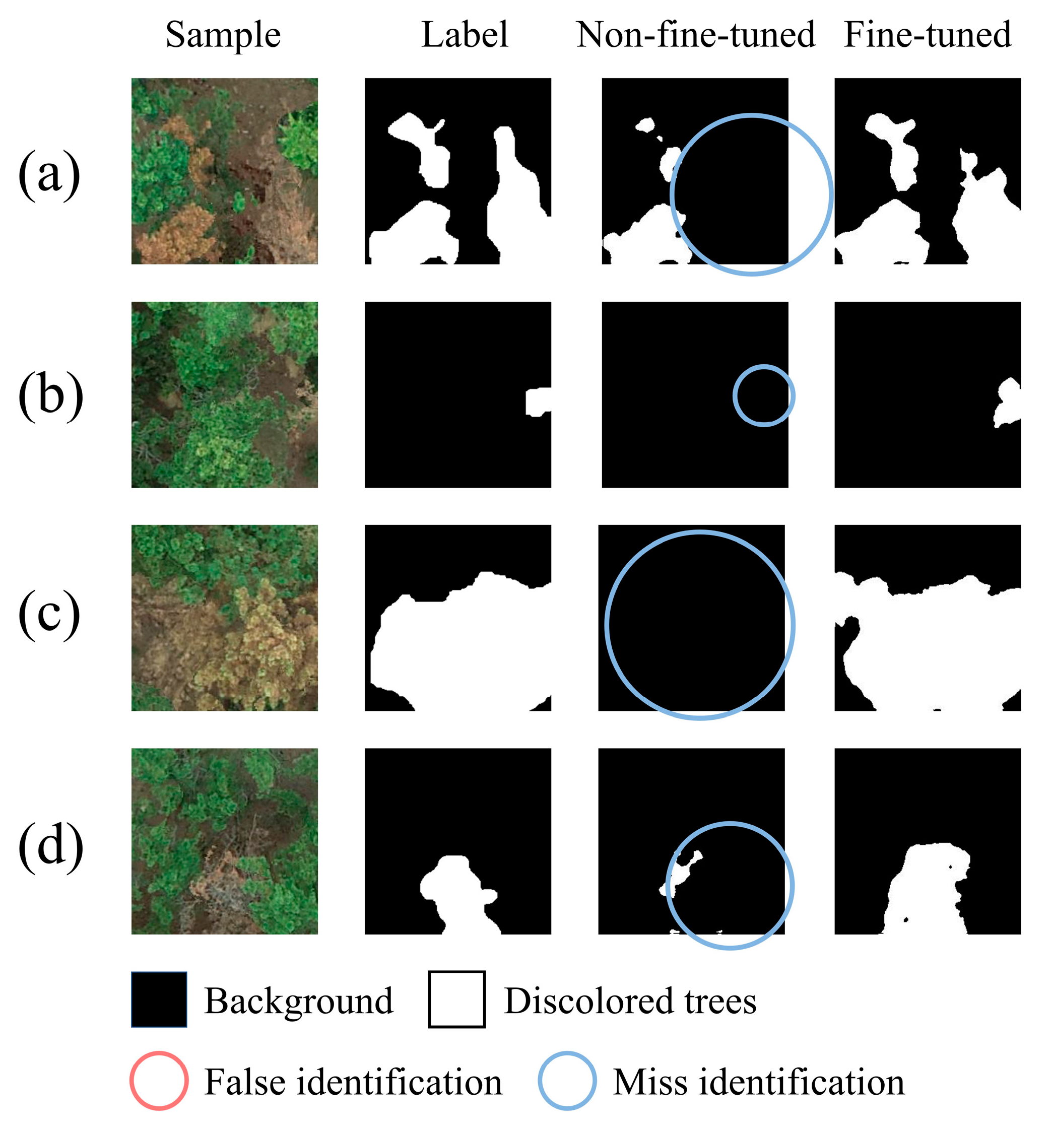
3.3. Model Fine-Tuning Study

In previous experiments, EVitNet was sufficiently trained on Dataset A, but its direct application for prediction on Dataset B yielded poor accuracy. On Dataset A, the single-category IoU for discolored trees segmentation was as high as 0.7134, while on Dataset B, the IoU dropped to 0.321. All models used for comparison in this study exhibited this phenomenon. On the one hand, this is due to the insufficient generalization ability of the models. On the other hand, it is because there are significant differences in sampling sensors, height, and terrain between the two datasets, leading to substantial differences in the distribution of feature information. In this study, an experiment for model fine-tuning was designed, with a series of training sample sizes set according to gradients and three different model fine-tuning strategies, yielding the corresponding experimental results (Figure 9).
The experimental results indicated that, due to the significant differences between the two datasets, the final model achieved the highest accuracy when fine-tuning without freezing the backbone network. For global fine-tuning, when the number of new samples used for training was more than 30%, the accuracy generally reached a relatively high level, which is higher than the IoU of the baseline model UNet (0.669).

3.4. Ablation Study

To assess the contribution of each component to the network accurately, ablation experiments were conducted. The MobileVit Block, MobileNetv2 block, ExpConv decoder, and fine-tuning learning were taken as the four basic factors. All training was carried out with the hyperparameter settings consistent with those in Section 3.3. IoU, F1 score, precision, and recall were used as the performance evaluation metrics for the models, where IoU_B refers to the IoU obtained when testing on Dataset B. The following ablation experiments were performed, and the experimental results are shown in Table 4.
Ablation of MobileViT Block: To lighten the model, the bottleneck part of the network was removed to reduce redundant channels in feature maps. This prevented the number of parameters from increasing exponentially with network depth, significantly reducing the network’s parameter count and computational load. To enhance the network’s ability to fuse global features, a lightweight ViT structure was introduced starting from the fourth encoder in the backbone network. This effectively improved segmentation accuracy while keeping the parameter size small. As shown in Table 3, compared to Unet, Unet + MobileViT has 23.65 M fewer parameters and a 1.8% increase in segmentation IoU. This indicates that redesigning the number of channels and incorporating a lightweight ViT can not only reduce the model’s parameter count but also improve the accuracy of identifying PWD-affected discolored trees.
Ablation of MobileNetv2 Block: To further improve the efficiency of feature extraction in the backbone network, the more efficient convolution module, MobileNetv2 Block, was used to replace standard convolutions. This slightly reduced the number of parameters and further enhanced the network’s segmentation accuracy. As shown in Table 3, the segmentation IoU increased by 2.2%, and the number of parameters decreased by 0.126 M. This suggests that, compared to standard convolutions, the MobileNetv2 Block is more suitable for the task of identifying PWD-affected discolored trees.
Ablation of Expanded Convolution in Decoder: Expanded convolutions were used to improve the accuracy of the model during the upsampling phase without increasing the number of network parameters. The standard convolution blocks after each decoder were replaced with expanded convolution blocks. As shown in Table 3, compared to Unet + MobileViT + Mv2, EVitNet achieved a slight improvement in segmentation accuracy. The idea behind expanded convolutions is similar to that of the MobileViT Block: Both expand the features, perform computations, and then compress them back to their original dimensions. This approach is very effective for the task of discolored trees identification.
Ablation of Model Fine-tuning: Among the various ablation experiments, the IoU_B on Dataset B was relatively low, indicating that the model trained on Dataset A could not be directly used to predict Dataset B. As shown in Table 3, after fine-tuning with a small portion of samples, EVitNet was able to achieve high accuracy on Dataset B.

4. Discussions

4.1. Network Performance Analysis

Currently, research on semantic segmentation methods for the identification of discolored trees is gradually increasing. Zhang et al. [39] were the first to attempt using segmentation methods for the recognition of discolored trees, comparing the Random Forest and U-Net algorithms. The latter, based on a CNN, can extract features more effectively and showed an absolute advantage in recognition accuracy. Li et al. [40] proposed an improved Mask R-CNN instance segmentation method for identifying discolored trees at various infection stages, achieving an overall accuracy of 71%. Zhi et al. [41] compared several algorithms, including U-Net, DeepLabv3+, FPN, and SAM, and found that UNet achieved the highest accuracy on discolored tree datasets in RGB, HSV, and mixed modes. Their research mainly compared and evaluated mainstream networks on their self-built discolored tree dataset. In contrast, our study not only assessed mainstream network performance on our self-built dataset but also proposed a new lightweight algorithm and used fine-tuning to address generalization issues. Due to dataset differences, direct comparison is not feasible. So, we reproduced their methods on our dataset for comparison, with the results presented in the earlier Results Section. These results echoed their findings, with UNet showing the highest accuracy among mainstream networks. In the task of identifying PWD-affected discolored trees, EVitNet significantly outperforms mainstream segmentation networks. The challenge of this task lies in distinguishing discolored tree lesions from similar ground objects. The uniqueness of EVitNet lies in its lightweight EasyVit backbone network, which combines a CNN and a Transformer. A CNN is responsible for extracting and processing local features to ensure precise segmentation boundaries, while a Transformer processes features from a global perspective to ensure accurate classification of pixel categories. Additionally, the idea of flattening the feature map, performing operations, and then contracting it is adopted in multiple parts of the network, saving parameter overhead and improving accuracy. In EVitNet, in addition to the residual connections between the encoder and decoder, residual connections are also used in the MV2 Block and MobileVit Block, preserving rich local detail features and ultimately achieving accurate semantic segmentation of discolored tree lesions.
Using the same hyperparameter settings as in Section 3.3 and the same training and testing samples, each model was trained for prediction, yielding the segmentation results for PWD-affected discolored trees. Figure 10 shows the segmentation results of representative samples under different lighting conditions and complexities. Five semantic segmentation models, PSPNet, Segformer, DeepLabv3+, HrNet, and Swin-Unet, were used for comparison.
In Figure 10, for sample (a), the contrast is clear, and there is little environmental interference, so all models are able to identify the discolored trees. However, DeepLabv3+ missed some pixels of the discolored trees. In samples (b), (c), and (d), due to strong environmental interference, poor lighting, and other reasons, many models had a large number of missed and false detections. The EVitNet proposed in this study has the best robustness, with only a small number of pixels missed or falsely detected. It can be seen that there are still some discrepancies between the EVitNet results and the label. These discrepancies correspond to the misclassified pixels. In addition to the pixels near the discolored tree lesions, there are also a few misclassified pixels in the background. For example, in sample (b), EVitNet misclassified some pixels on the roof as discolored trees. In the sample in sample (c), there is also a small portion of missed detections. However, these types of errors occur in all models, and there is currently no way to optimize them. Further research in the future is needed.
In this study, fine-tuning the model had a significant impact on the network’s segmentation performance. The comparison of the segmentation results before and after fine-tuning can be seen in Figure 11. The non-fine-tuned model refers to using EVitNet trained on Dataset A directly to identify samples in Dataset B, while the fine-tuned model refers to using EVitNet after fine-tuning with 40% of the training set to identify samples in Dataset B.
It can be seen from Figure 11 that the non-fine-tuned model has a serious problem of missed detection, but there are almost no false positives. This is because in the task of discolored trees recognition, most areas of the samples are negative samples. When the model encounters pixels it cannot recognize during the identification process, it is more likely to classify them into the background category. Additionally, some knowledge learned by the model on Dataset A is also applicable to Dataset B, so there are almost no false positives. After fine-tuning, the model’s missed detection rate dropped significantly, and the recognition accuracy reached a high level. Fine-tuning the model has greatly enhanced the practicality of EVitNet in different scenarios.

4.2. Advantages and Disadvantages

The quality of training samples has a significant impact on the model’s accuracy. The task of this study is to segment the discolored tree lesions. Training excessively on negative samples can adversely affect the model’s precision. Experiments have shown that training solely with samples containing discolored tree lesions yields a higher accuracy than using all samples. The datasets used in this study were annotated under the guidance of forestry disease experts, which, to some extent, excluded interference from discolored pine trees caused by non-PWD and other broad-leaved discolored trees. This allowed the model to learn from the experts’ judgment and experience. Currently, research on remote sensing monitoring of PWD-affected discolored trees mainly focuses on object detection algorithms. However, object detection algorithms represented by YOLO often miss small targets [42] and cannot precisely identify partially diseased branches and leaves of a single pine tree. Semantic segmentation models have lower requirements for image spatial resolution and are more suitable for large-scale monitoring of discolored trees. They can detect discolored trees earlier and more comprehensively. Moreover, the EVitNet proposed in this study has fewer parameters than the YOLO series of object detection algorithms. The research results of Xia et al. [43] indicate that an excessive number of network layers does not enhance the accuracy of segmentation but merely increases the computational load, so this study used a lightweight ViT to enhance the network’s ability to process global features, and the segmentation network was lightened, making the network complexity match the sample complexity. The images of PWD infected trees have low contrast and limited local spatial information. Traditional CNNs can only capture local features and ignore long-range pixel relationships, lacking global perception. This makes it hard to classify pixels based on the entire image context, especially when lesions are scattered. Global feature fusion can highlight key areas, and combining with local features improves segmentation accuracy. Using a Transformer for feature extraction solves the global perception issue but increases parameters, hindering widespread deployment. EVitNet combines the strengths of CNNs and Transformers, uses fewer channels, introduces a Transformer in deeper layers, shortens the self-attention sequence length, and significantly reduces parameters and computational complexity, achieving a balance between speed and accuracy. Additionally, we deployed EVitNet on the NVIDIA Jetson XAVIER NX developer kit. On this platform, the unquantized algorithm achieved a segmentation speed of 74.88 fps, with a peak instantaneous power consumption of 14.3 W and an average power consumption of 10.2 W. Using real-time semantic segmentation algorithms can improve the workflow of discovering and locating discolored trees and can timely curb the spread of PWD.
Although EVitNet performed well on the PWD-affected discolored trees dataset, the lightweight design reduced some parameters and lowered the model complexity, which may result in a gap between this model and SOTA algorithms in other fields. The EVitNet model was designed for discolored tree datasets and excels at segmenting similar lesion-type images. However, its performance in other real-world scenarios may be suboptimal. This study focused on identifying only one type of target with relatively simple and low-resolution image content. In contrast, real-world scenes often have more target varieties, complexity, and higher resolutions. The inconsistent feature distribution means the lightweight backbone network EasyVit used in this study may fail to extract sufficient features, leading to potential poor segmentation accuracy in other scenarios, which might restrict the algorithm’s applicability. It may only be suitable for tasks with similar complexity to PWD-affected discolored trees identification, such as cotton root rot, bacterial blight of rice, and powdery mildew in wheat [44,45]. In addition, the PWN can infect 57 species of pine plants and 13 non-pine species [46]. Annotating data for training semantic segmentation models has always been difficult. The fine-tuning learning method used in this study greatly improved the model’s segmentation performance on new datasets, but the new data still needs to be annotated, which is very time-consuming in the workflow of identifying discolored trees and is not conducive to accelerating the process. Further research is needed to find new methods to improve the model’s performance on new datasets.

5. Conclusions

The aims of this study were to overcome the limitations of current semantic segmentation technologies in recognizing discolored trees, such as the lack of specialized algorithms and sub-par performance of mainstream methods in accuracy, speed, and robustness in complex environments. We believe that precise annotation and more efficient segmentation networks can boost recognition accuracy. Thus, we propose creating a high-quality dataset, developing the EVitNet model with a lightweight ViT encoder and CNN decoder, and determining the optimal fine-tuning strategy. The EasyVit backbone has low parameter overhead and improves feature extraction in complex environments. The decoder, using expended convolutions, slightly improves segmentation accuracy without adding parameters. The fine-tuning learning method effectively tackles generalization challenges from different environments and sensors. The model can achieve high accuracy on new datasets with only a few new samples. It has an IoU of 0.713, an F1 score of 0.833, a segmentation speed of 850.43 fps, and 1.195 M parameters. EVitNet excels in recognizing discolored trees and can semantically segment PWD-affected trees accurately and efficiently. As PWD is sporadic in many regions, monitoring is crucial for control. This study offers technical support for faster and more accurate remote sensing monitoring. However, as mentioned in the limitations, the EvitNet may only achieve high accuracy on feature-similar datasets. Future work could explore its application to other data types, such as multispectral and hyperspectral samples. Additionally, semi-supervised or unsupervised learning could be considered to address the difficulty of dataset annotation.

Author Contributions

Q.W.: Methodology, Software, Formal analysis, Writing—original draft, Writing—review and editing. M.C.: Validation, Resources, Funding acquisition. H.S.: Validation, Investigation. T.Y.: Validation, Investigation. G.X.: Validation, Investigation. W.W.: Validation, Investigation. C.Z.: Validation, Resources, Funding acquisition. R.Z.: Conceptualization, Validation, Investigation, Resources, Project administration, Funding acquisition. All authors have read and agreed to the published version of the manuscript.

Funding

This work was supported by the Promotion and Innovation Project of Beijing Academy of Agriculture and Forestry Sciences (KJCX20230205), the Major Scientific and Technological Achievements Cultivation Project of BAAFS, the National Natural Science Foundation of China (32071907) and the National Key R & D Program of China (2021YFD1400900).

Data Availability Statement

The code can be accessed on GitHub via https://github.com/ib00r/EVitNet (accessed on 25 March 2025), and the datasets used in the current study are available from the corresponding author upon reasonable request.

Acknowledgments

We would like to thank all contributors to this article and all reviewers who provided very constructive and helpful comments to improve the manuscript.

Conflicts of Interest

The authors declare no conflicts of interest.

Abbreviations

The following abbreviations are used in this manuscript:
DOAJDirectory of open access journals
TLAThree-letter acronym
LDLinear dichroism

References

  1. Fonseca, L.; Silva, H.; Cardoso, J.M.S.; Esteves, I.; Maleita, C.; Lopes, S.; Abrantes, I. Bursaphelenchus xylophilus in Pinus sylvestris—The First Report in Europe. Forests 2024, 15, 1556. [Google Scholar] [CrossRef]
  2. Hu, G.; Wang, T.; Wan, M.; Bao, W.; Zeng, W. UAV remote sensing monitoring of pine forest diseases based on improved Mask R-CNN. Int. J. Remote Sens. 2022, 43, 1274–1305. [Google Scholar] [CrossRef]
  3. Wang, Y.; Chen, H.; Wang, J.; Li, D.; Wang, H.; Jiang, Y.; Fei, X.; Sun, L.; Li, F. Research progress on the resistance mechanism of host pine to pine wilt disease. Plant Pathol. 2024, 73, 469–477. [Google Scholar] [CrossRef]
  4. Zhang, K.; Liang, J.; Yan, D.; Zhang, X. Research Advances of Pine Wood Nematode Disease in China. World For. Res. 2010, 23, 59–63. [Google Scholar]
  5. Announcement of the National Forestry and Grassland Administration (No. 7 of 2023) (Pine Wood nematode Disease Epidemic Area in 2023). Available online: https://www.forestry.gov.cn/c/www/gkzfwj/380005.jhtml (accessed on 4 November 2024).
  6. Xie, W.; Wang, H.; Liu, W.; Zang, H. Early-Stage Pine Wilt Disease Detection via Multi-Feature Fusion in UAV Imagery. Forests 2024, 15, 171. [Google Scholar] [CrossRef]
  7. Li, M.; Li, H.; Ding, X.; Wang, L.; Wang, X.; Chen, F. The Detection of Pine Wilt Disease: A Literature Review. Int. J. Mol. Sci. 2022, 23, 10797. [Google Scholar] [CrossRef]
  8. Ye, J. Epidemic Status of Pine Wilt Disease in China and Its Prevention and Control Techniques and Counter Measures. Sci. Silvae Sin. 2019, 55, 1–10. [Google Scholar]
  9. Zhao, J.; Huang, J.; Yan, J.; Fang, G. Economic Loss of Pine Wood Nematode Disease in Mainland China from 1998 to 2017. Forests 2020, 11, 1042. [Google Scholar] [CrossRef]
  10. Chen, Z.; Lin, H.; Bai, D.; Qian, J.; Zhou, H.; Gao, Y. PWDViTNet: A lightweight early pine wilt disease detection model based on the fusion of ViT and CNN. Comput. Electron. Agric. 2025, 230, 109910. [Google Scholar] [CrossRef]
  11. Koy, A.; Çolak, A.B. The Intraday High-Frequency Trading with Different Data Ranges: A Comparative Study with Artificial Neural Network and Vector Autoregressive Models. AAES 2023, 2, 123–133. [Google Scholar] [CrossRef]
  12. Purohit, J.; Dave, R. Leveraging Deep Learning Techniques to Obtain Efficacious Segmentation Results. AAES 2023, 1, 11–26. [Google Scholar] [CrossRef]
  13. Chiphiko, B.A.; Kim, H.; Ali, P.; Eneya, L. Forward Secrecy Attack on Privacy-Preserving Machine Authenticated Key Agreement for Internet of Things. AAES 2025, 3, 29–34. [Google Scholar] [CrossRef]
  14. Andreychev, A.V.; Lapshin, A.S.; Kuznetcov, V.A. Techniques for recording the Eagle Owl (Bubo bubo) based on vocal activity. Zool. Zhurnal 2017, 96, 601–605. [Google Scholar] [CrossRef]
  15. Zhang, M.; Yuan, C.; Liu, Q.; Liu, H.; Qiu, X.; Zhao, M. Detection of mulberry leaf diseases in natural environments based on improved YOLOv8. Forests 2024, 15, 1188. [Google Scholar] [CrossRef]
  16. Stone, C.; Mohammed, C. Application of Remote Sensing Technologies for Assessing Planted Forests Damaged by Insect Pests and Fungal Pathogens: A Review. Curr. For. Rep. 2017, 3, 75–92. [Google Scholar] [CrossRef]
  17. Dash, J.P.; Watt, M.S.; Pearse, G.D.; Heaphy, M.; Dungey, H.S. Assessing very high resolution UAV imagery for monitoring forest health during a simulated disease outbreak. ISPRS J. Photogramm. Remote Sens. 2017, 131, 1–14. [Google Scholar] [CrossRef]
  18. Tao, H.; Li, C.; Zhao, D.; Deng, S.; Hu, H.; Xu, X.; Jing, W. Deep learning-based dead pine tree detection from unmanned aerial vehicle images. Int. J. Remote Sens. 2020, 41, 8238–8255. [Google Scholar] [CrossRef]
  19. Wang, W.; You, Z.; Shao, L.; Li, X.; Wu, S.; Zhang, Z.; Huang, S.; Zhang, F. Recognition of dead pine trees using YOLOv5 by super-resolution reconstruction. Nongye Gongcheng XuebaoTransactions Chin. Soc. Agric. Eng. 2023, 39, 137–145. [Google Scholar] [CrossRef]
  20. Ye, X.; Pan, J.; Shao, F.; Liu, G.; Lin, J.; Xu, D.; Liu, J. Exploring the potential of visual tracking and counting for trees infected with pine wilt disease based on improved YOLOv5 and StrongSORT algorithm. Comput. Electron. Agric. 2024, 218, 108671. [Google Scholar] [CrossRef]
  21. Zhang, P.; Wang, Z.; Rao, Y.; Zheng, J.; Zhang, N.; Wang, D.; Zhu, J.; Fang, Y.; Gao, X. Identification of Pine Wilt Disease Infected Wood Using UAV RGB Imagery and Improved YOLOv5 Models Integrated with Attention Mechanisms. Forests 2023, 14, 588. [Google Scholar] [CrossRef]
  22. Long, J.; Shelhamer, E.; Darrell, T. Fully Convolutional Networks for Semantic Segmentation. arXiv 2018, arXiv:1411.4038. [Google Scholar]
  23. Ronneberger, O.; Fischer, P.; Brox, T. U-Net: Convolutional Networks for Biomedical Image Segmentation. arXiv 2015, arXiv:1505.04597. [Google Scholar]
  24. Chen, L.-C.; Zhu, Y.; Papandreou, G.; Schroff, F.; Adam, H. Encoder-Decoder with Atrous Separable Convolution for Semantic Image Segmentation. arXiv 2018, arXiv:1802.02611. [Google Scholar]
  25. Vaswani, A.; Shazeer, N.; Parmar, N.; Uszkoreit, J.; Jones, L.; Gomez, A.N.; Kaiser, L.; Polosukhin, I. Attention Is All You Need. arXiv 2023, arXiv:1706.03762. [Google Scholar]
  26. Kirillov, A.; Mintun, E.; Ravi, N.; Mao, H.; Rolland, C.; Gustafson, L.; Xiao, T.; Whitehead, S.; Berg, A.C.; Lo, W.-Y.; et al. Segment Anything. In Proceedings of the 2023 IEEE/CVF International Conference on Computer Vision (ICCV), Paris, France, 1–6 October 2023; pp. 3992–4003. [Google Scholar] [CrossRef]
  27. Zhu, C.; Xu, Y.; Zhang, M.; Chen, J.; Li, S. Structure Characteristics of Pinus thunbergii Stand in Laoshan Mountain of Qingdao City. For. Inventory Plan. 2019, 44, 33–39. [Google Scholar] [CrossRef]
  28. Zhou, J.; Xing, S.; Han, C.; Zhang, F.; Zhao, M.; Liu, X. Analysis on Storm Surge Resistant Ability of Different Pine Tree Species. J. Southwest. For. Univ. 2009, 4, 26–28. [Google Scholar] [CrossRef]
  29. Hao, Z.; Huang, J.; Li, X.; Sun, H.; Fang, G. A multi-point aggregation trend of the outbreak of pine wilt disease in China over the past 20 years. For. Ecol. Manag. 2022, 505, 119890. [Google Scholar] [CrossRef]
  30. Shorten, C.; Khoshgoftaar, T.M. A survey on Image Data Augmentation for Deep Learning. J. Big Data 2019, 6, 60. [Google Scholar] [CrossRef]
  31. Liu, H.; Li, W.; Jia, W.; Sun, H.; Zhang, M.; Song, L.; Gui, Y. Clusterformer for Pine Tree Disease Identification Based on UAV Remote Sensing Image Segmentation. IEEE Trans. Geosci. Remote Sens. 2024, 62, 1–15. [Google Scholar] [CrossRef]
  32. Mehta, S.; Rastegari, M. MobileViT: Light-weight, General-purpose, and Mobile-friendly Vision Transformer. arXiv 2022, arXiv:2110.02178. [Google Scholar]
  33. Sandler, M.; Howard, A.; Zhu, M.; Zhmoginov, A.; Chen, L.-C. MobileNetV2: Inverted Residuals and Linear Bottlenecks. arXiv 2019, arXiv:1801.04381. [Google Scholar]
  34. Liu, S.; Li, C.; Nan, N.; Zong, Z.; Song, R. MMDM: Multi-Frame and Multi-Scale for Image Demoireing. arXiv 2020, arXiv:1909.11947. [Google Scholar]
  35. Zhao, H.; Shi, J.; Qi, X.; Wang, X.; Jia, J. Pyramid Scene Parsing Network, in: 2017 IEEE Conference on Computer Vision and Pattern Recognition (CVPR). In Proceedings of the 2017 IEEE Conference on Computer Vision and Pattern Recognition (CVPR), Honolulu, HI, USA, 21–26 July 2017; pp. 6230–6239. [Google Scholar] [CrossRef]
  36. Xie, E.; Wang, W.; Yu, Z.; Anandkumar, A.; Alvarez, J.M.; Luo, P. SegFormer: Simple and Efficient Design for Semantic Segmentation with Transformers. arXiv 2021, arXiv:2105.15203. [Google Scholar]
  37. Wang, J.; Sun, K.; Cheng, T.; Jiang, B.; Deng, C.; Zhao, Y.; Liu, D.; Mu, Y.; Tan, M.; Wang, X.; et al. Deep High-Resolution Representation Learning for Visual Recognition. IEEE Trans. Pattern Anal. Mach. Intell. 2021, 43, 3349–3364. [Google Scholar] [CrossRef]
  38. Cao, H.; Wang, Y.; Chen, J.; Jiang, D.; Zhang, X.; Tian, Q.; Wang, M. Swin-Unet: Unet-like Pure Transformer for Medical Image Segmentation. arXiv 2021, arXiv:2105.05537. [Google Scholar]
  39. Zhang, R.; Xia, L.; Chen, L.; Xie, C.; Chen, M.; Wang, W. Recognition of wilt wood caused by pine wilt nematode based on U-Net network and unmanned aerial vehicle images. Trans. CSAE 2020, 36, 61–68. [Google Scholar] [CrossRef]
  40. Li, H.; Chen, L.; Yao, Z.; Li, N.; Long, L.; Zhang, X. Intelligent Identification of Pine Wilt Disease Infected Individual Trees Using UAV-Based Hyperspectral Imagery. Remote Sens. 2023, 15, 3295. [Google Scholar] [CrossRef]
  41. Zhi, J.; Li, L.; Zhu, H.; Li, Z.; Wu, M.; Dong, R.; Cao, X.; Liu, W.; Qu, L.; Song, X.; et al. Comparison of Deep Learning Models and Feature Schemes for Detecting Pine Wilt Diseased Trees. Forests 2024, 15, 1706. [Google Scholar] [CrossRef]
  42. Yu, R.; Luo, Y.; Zhou, Q.; Zhang, X.; Wu, D.; Ren, L. Early detection of pine wilt disease using deep learning algorithms and UAV-based multispectral imagery. For. Ecol. Manag. 2021, 497, 119493. [Google Scholar] [CrossRef]
  43. Xia, L.; Zhang, R.; Chen, L.; Li, L.; Yi, T.; Wen, Y.; Ding, C.; Xie, C. Evaluation of Deep Learning Segmentation Models for Detection of Pine Wilt Disease in Unmanned Aerial Vehicle Images. Remote Sens. 2021, 13, 3594. [Google Scholar] [CrossRef]
  44. Zhang, J.; Huang, Y.; Pu, R.; Gonzalez-Moreno, P.; Yuan, L.; Wu, K.; Huang, W. Monitoring plant diseases and pests through remote sensing technology: A review. Comput. Electron. Agric. 2019, 165, 104943. [Google Scholar] [CrossRef]
  45. Yang, C. Remote Sensing and Precision Agriculture Technologies for Crop Disease Detection and Management with a Practical Application Example. Engineering 2020, 6, 528–532. [Google Scholar] [CrossRef]
  46. Jiang, M.; Huang, B.; Yu, X.; Zheng, W.; Jin, Y.; Liao, M.; Ni, J. Distribution, Damage and Control of Pine Wilt Disease. J. Zhejiang Sci. Technol. 2018, 6, 83–91. [Google Scholar] [CrossRef]
Figure 1. The study area, which is in Shandong province, China, and some orthophotos created from the collected data. (a) Partial orthophoto images sampled in Qingdao, Shandong Province; (b) Map of the study area.
Forests 16 00596 g001
Figure 2. A subset of affected tree samples, including a few samples from Dataset A and Dataset B. (ad) show samples with severe interference; (eh) show samples with different lesion size; (il) show samples with different shapes; (mp) show samples in different lighting conditions; (qt) show samples from dataset B.
Forests 16 00596 g002
Figure 3. Illustration of data augmentation effects on PWD-affected tree sample. (a) The original image. (b) The original image was transformed from RGB color space to the HSV (Hue, Saturation, and Value) color space, followed by random adjustments (0.9~1.1 times of original). (c) The original image was subjected to random horizontal and vertical flips (50% probability). (d) The original image was subjected to random blurring (20% probability of Gaussian blur). (e) Randomly add gray strips to the original image (width 0–50 pixels). (f) The aspect ratio of the original image was randomly adjusted, followed by gray padding at the edges (height and width resize to 0.7–1.3 times of original, and rescale to 256 × 256). (g) The original image was subjected to random rotation, followed by gray padding at the edges (0–90 degrees, 50% probability).
Forests 16 00596 g003
Figure 4. The architecture of the lightweight algorithm, EViTNet, which is based on CNN-Transformer.
Forests 16 00596 g004
Figure 5. Contrast diagram between expanded convolution and ordinary convolution. Although the convolution process is different, the resulting feature map can be equivalent.
Forests 16 00596 g005
Figure 6. Model fine-tuning flow diagram, which shows the entire training process. There are three kinds of fine-tuning tactics in the experiment, involving freeze backbone, partial freeze, and global fine-tuning.
Forests 16 00596 g006
Figure 7. Scatter bubble diagram for comparison of performance of mainstream models, which shows that EVitNet reaches the highest accuracy and maintains a fast speed.
Forests 16 00596 g007
Figure 8. (a) Training loss and (b) validation loss curves of each model, indicating that all models have converged.
Forests 16 00596 g008
Figure 9. Comparison of three model fine-tuning strategies, which shows that global fine-tuning is the best strategy, and the accuracy reaches the highest when the learning quantity is around 30%.
Forests 16 00596 g009
Figure 10. The visualization segmentation results of mainstream models, which shows that misses and false identifications occur least in EVitNet. (a) shows the visual result of a sample in sufficient light; (b) shows the visual result of a sample with interference form background with similar color and texture; (c) shows the visual result of a sample with multiple lesions of different shapes; (d) shows the visual result of a sample in insufficient light.
Forests 16 00596 g010
Figure 11. The visualization segmentation results of the non-fine-tuned model and the fine-tuned model, showing that fine-tuning can greatly improve the accuracy of the model on a new dataset. (a) Visual results of a sample with multiple lesions; (b) Visual results of a sample with small target; (c) Visual results of a sample with large target; (d) Visual results of a sample with target of medium size.
Forests 16 00596 g011
Table 1. Details of Dataset A and Dataset B.
Dataset ADataset B
Collection systemForests 16 00596 i001
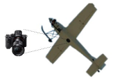
DB-II + Snoy alpha 7 R II
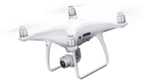
Forests 16 00596 i002
DJI Phantom 4 Pro
Resolution of raw data7952 × 53045472 × 3648
Amount of raw data17,0001096
Area200 km20.7 km2
LocationQingdao, ShandongYantai, Shandong
Principal speciesPinus densifloraPinus densiflora
and Pinus thunbergii
Table 2. Comparison of different training sets and loss functions.
Training SchemeIoUdiscoloredtreeIoUbackgroundF1 ScorePrecisionRecallTime
original training set0.5100.9970.6760.8460.5638.4 h
original training set + focal loss0.6170.9970.7630.8080.7227.4 h
filtered training set0.6470.9960.8040.7150.8712.1 h
filtered training set + focal loss0.6680.9970.8020.7970.8072.0 h
The bold data in the table represents the optimal value in its respective column.
Table 3. Performance comparison of mainstream models.
ModelBackboneIoUF1 ScorePrecisionRecallParams (M)GFLOPsFPS
UNet (Baseline)vgg0.6690.8000.7930.80824.981112.91839.81
DeepLabv3+mobilenet0.4720.6450.5880.7155.81853.026100.45
HrNethrnetv2_w180.5610.7110.7830.6519.64232.948211.19
PSPNetmobilenet0.6170.7600.8190.7082.3776.034886.50
SegformerSegformer_b00.6550.7860.8120.7683.72013.696485.17
Swin-UnetSwin-Unet0.6650.7990.8170.78198.3026.33162.43
EVitNet (Ours)EasyVit0.7130.8330.8530.8141.1951.636850.43
In the table, the bold data in the table represents the optimal value in its respective column.
Table 4. The result of ablation study.
AblationMobileVitMv2ExpCovFine-TurningIoUIoU_BF1 ScorePrecisionRecallParams
(M)
GFLOPsFPS
Unet(baseline) 0.6690.1090.8000.7930.80824.981112.91839.81
Unet+MobileVit 0.6870.2110.8160.8190.8121.3311.937771.76
Unet+MobileVit+Mv2 0.7090.2970.8300.8350.8251.1951.636839.28
Unet+MobileVit+Mv2+ExpConv(EVitNet) 0.7130.3210.8330.8530.8141.1951.636850.43
Unet+MobileVit+Mv2+ExpConv+fine-turning0.2950.7350. 4700.3140.8311.1951.636845.69
In the table, the checks from the 2nd to the 5th columns show whether a module is used. In the following columns, bold numbers indicate the optimal value in that column.
Disclaimer/Publisher’s Note: The statements, opinions and data contained in all publications are solely those of the individual author(s) and contributor(s) and not of MDPI and/or the editor(s). MDPI and/or the editor(s) disclaim responsibility for any injury to people or property resulting from any ideas, methods, instructions or products referred to in the content.

