Hyperspectral Remote Sensing Estimation and Spatial Scale Effect of Leaf Area Index in Moso Bamboo (Phyllostachys pubescens) Forests Under the Stress of Pantana phyllostachysae Chao

Abstract

Leaf area index (LAI) serves as a crucial indicator for assessing vegetation growth status, and unmanned aerial vehicle (UAV) optical remote sensing technology provides an effective approach for forest pest-related research. This study investigated the feasibility of LAI estimation in Moso bamboo (Phyllostachys pubescens) forests with different damage levels using UAV data while simultaneously exploring the scale effects of various spatial resolutions. Through image resampling using 10 distinct spatial resolutions and field data classification based on Pantana phyllostachysae Chao pest severity (healthy and mild damaged as Scheme 1, moderate damaged and severe damaged as Scheme 2, and all as Scheme 3), three machine learning algorithms (SVM, RF, and XGBoost) were employed to establish LAI estimation models for both single and mixed damage levels. Comparative analysis was conducted across different schemes, algorithms, and spatial resolutions to identify optimal estimation models. The results showed that (1) XGBoost-based regression models achieved superior performance across all schemes, with optimal model accuracy consistently observed at 3 m spatial resolutions; (2) minimal scale effects occurred at a 3 m resolution for Schemes 1 and 2, while Scheme 3 showed lowest scale effects at 1.5 m followed by 3 m resolutions; (3) Scheme 3 exhibited significant advantages in mixed damaged bamboo forest inversion with robust performance across all damage levels, whereas Schemes 1 and 2 demonstrated higher accuracy for single damaged scenarios compared to mixed damaged. This research validates the feasibility of incorporating pest stress factors into LAI estimation through different pest damage models, offering novel perspectives and technical support for parameter inversion in Moso bamboo forests.

1. Introduction

As a native herbaceous species in forest ecosystems, bamboo constitutes a globally significant forest type characterized by its aggressive expansion through extensive rhizome networks, leading to continuous bamboo forest expansion. These expansions are predominantly distributed across Asian and subtropical regions. In China, Moso bamboo (Phyllostachys pubescens Mazel ex Houzeau de Lehaie) stands as the most economically vital bamboo species, distinguished by its vast cultivation area, wide geographical distribution, and exceptional socioeconomic value. This species demonstrates remarkable production potential through versatile applications in construction, manufacturing, and ecological services, generating substantial economic returns. However, the health of Moso bamboo forests faces severe threats from biotic stressors, particularly the folivorous pest Pantana phyllostachysae Chao (P. phyllostachysae). The larval feeding activity causes progressive defoliation, triggering a critical decline in leaf biomass that directly reduces the leaf area index (LAI). This defoliation process not only compromises bamboo photosynthetic capacity and ecosystem stability but also results in measurable economic losses across upstream cultivation and downstream processing industries.

The LAI, originally conceptualized by British agroecologist Watson [1], serves as a critical biophysical parameter for investigating plant canopy functional processes and vegetation growth dynamics [2]. Established measurement methodologies encompass direct approaches (e.g., destructive sampling) and indirect techniques utilizing optical instruments such as the LAI-2200 Plant Canopy Analyzer (American Li-Cor, Lincoln, NE, USA) [3,4]. As an important structural parameter of plants, LAI has been extensively applied in forestry and agriculture studies, proving instrumental in stand quality assessment, crop yield prediction, and pest impact evaluation [5,6,7,8,9,10,11]. In the study of Moso bamboo diseases and pests, the LAI exhibits a decreasing trend with elevated P. phyllostachysae damage severity levels, effectively quantifying the impact of this specific pest on Moso bamboo forest [12]. The rapid advancement of drone technology has enabled remote sensing to break free from its traditional reliance on satellite imagery, with low-altitude, high-resolution remote sensing emerging as a mainstream approach in the field [6,13,14,15]. Recent advancements integrating pest stress factors into LAI inversion and biochemical component retrieval have shown significant accuracy improvements over conventional PROSAIL model approaches [16,17]. Satellite-based inversion extrapolates, such discrete values to estimate pixel-scale LAI, are applicable solely to homogeneous crop areas with uniform growth [18,19,20]. While these methods demonstrate high accuracy levels, they fail to address the spatial scale discrepancies inherent in instrument-based indirect LAI measurement scenarios. In UAV-based LAI inversion studies [21,22,23], while accurate plant-level LAI values can be obtained, these measurements only represent individual plants or plot averages. Similarly, forest LAI measurements (targeting tall species like arbor and fir) approximate stand-level LAI within specific ranges [11,24,25,26], yet this approach becomes ecologically invalid due to intra-stand heterogeneity, as single plots cannot represent pixel-scale variations. Due to the high resolution of UAV data, the pixels corresponding to LAI measurement points fail to fully encompass the entire plant canopy and may be projected onto surface features beneath forest canopy gaps, resulting in a reduction in the predictive capability of regression models. To address these limitations, Kamal et al. [27] identified 10 * 10 m as the optimal scale for mangrove LAI estimation; Revill et al. [28] addressed the spatial scale mismatch between ground-measured LAI and satellite imagery by utilizing UAV multi-spectral data as intermediate observations to reduce scale discrepancies, achieving over 50% improvement in both the coefficient of determination (R²) and error reduction.

Growing scholarly attention has focused on the impacts of spatial scale mismatches in research [29,30,31]. Within the context of Moso bamboo forest LAI studies, does spatial scale remain a non-negligible factor? This study employs high-spatial-resolution UAV imagery resampled into multiple lower-resolution tiers to develop algorithm-specific LAI estimation models using three machine learning approaches—support vector machine (SVM), random forest (RF), and extreme gradient boosting (XGBoost)—based on 332 predictive variables encompassing raw spectral bands, spectral indices, and texture features. The study concurrently examines pest infestation severity impacts on LAI retrieval accuracy while determining the optimal spatial scale for Moso bamboo forest LAI inversion. This research will examine the impacts of pest damage on Moso bamboo forest LAI, establishing a scientifically robust theoretical framework and technical reference system for LAI retrieval in subsequent studies.

2. Materials and Methods

2.1. Study Area

We took Shunchang County, Nanping City, Fujian Province, China, as the study area, located in the northwest of Fujian Province, featuring a subtropical monsoon climate with abundant sunlight and rainfall. With a bamboo forest area exceeding 44,000 hectares, Shunchang County is recognized as a national demonstration county for precise forest quality improvement, a strategic timber reserve base, and one of the first “Hometowns of Bamboo”. However, over the past decade, the bamboo forests in Shunchang County have been significantly impacted by pest infestations, primarily caused by the P. phyllostachysae. The affected area has shown a consistent upward trend, posing substantial threats to both the economic and ecological value of the bamboo forests.

In previous studies, research has been conducted on the remote sensing response capabilities, spread patterns, and pest impacts of bamboo forests under P. phyllostachysae infestation [32]. Among these, Li et al. [33] developed a model for extracting bamboo forest information. Building upon this research foundation, He et al. [34] proposed an innovative approach that integrated machine learning with a recursive feature elimination (RFE) algorithm to detect P. phyllostachysae bamboo pest infestations. The pest infestation levels are illustrated in Figure 1. Specifically, Area 1 is primarily characterized by moderate damage, while Area 2 is dominated by severe damage. In contrast, Area 3 is mainly characterized by healthy and mild damage.

2.2. Datasets and Preprocessing

2.2.1. Field Measured Point Data

During the terminal phase of the first generation, mid-phase of the second generation, and initial phase of the overwintering generation of Pantana phyllostachysae Chao, field measurements were conducted in the damaged Moso bamboo forest areas of Shunchang County. We measured the leaf area index (LAI) in survey plots by selecting areas with over 65% bamboo coverage using an LAI-2200 Plant Canopy Analyzer via indirect measurement. Since the LAI-2200 Plant Canopy Analyzer requires a measuring point (A) in an open area and point B under a forest area, the collected 66 points only satisfy two scheme combinations (healthy and mild, moderate, and severe). The operational procedure consisted of (1) installing a 45° view cap on the fisheye lens to prevent operator presence in the captured images; (2) measuring reference A-values in an open area within the instrument’s field of view; (3) obtaining four directional B-value measurements under the bamboo canopy. The instrument subsequently calculated the LAI value for each central measurement point. Centimeter-level precision GNSS positioning equipment was simultaneously employed to acquire geospatial coordinates, enabling precise correlation between LAI measurements and Moso bamboo forest in subsequent image analysis. Bamboo damage assessment followed established protocols from the “General Rules for Investigation of Major Forest Pests” (LY/T 2011-2012 [35]) and related industry standards. During the field sampling process, in addition to the aforementioned information, data were also collected on various bamboo forest parameters, including diameter at breast height, bamboo height, canopy density, age class distribution, and stand density. Furthermore, biochemical components such as leaf chlorophyll content and water content, as well as spectral information from leaves and soil, were also gathered.

2.2.2. Hyperspectral Image Acquisition and Processing of Moso Bamboo Forest Information

The utilized imagery data were collected by our research team during a field investigation in Dagan Town, Shunchang County on 23 October 2021. The main equipment used was a Ruisen unmanned aerial vehicle equipped with an HS-RPL hyperspectral sensor (

Table 1. HS-RPL main parameters of the airborne hyperspectral instrument.

Parameter Name	Parameter Value
Spectral region	400–1000 nm
Spectral resolution	2.1 nm
Spectral sampling rate	1.07 nm/5 nm
Carrying platform	RT650/DJI M600 Pro
Camera lens	18.5 mm, 23 mm
Spectral channel number	300
Spatial resolution	30 cm

). Flight surveys and ground data collection were conducted at an altitude of 90 m. After acquiring the images, the built-in SPECTRONON software of the Pika-L system was used to perform preprocessing steps such as radiometric correction, geometric correction, smoothing to reduce noise, and image clipping. The imagery encompasses two severely damaged bamboo sample plots and one healthy bamboo sample plot, covering a total area of 106,955.04 m².

In addition to the original spectra, other hyperspectral data-derived indicators are also the focus of this study for LAI inversion. These indicators primarily involve utilizing original spectra, spectral indices, and texture features to extract bamboo forest information characteristics from UAV hyperspectral data, thereby establishing LAI inversion models at various spatial resolutions.

The main acquisition and processing methods are as follows (Figure 2):

(1)

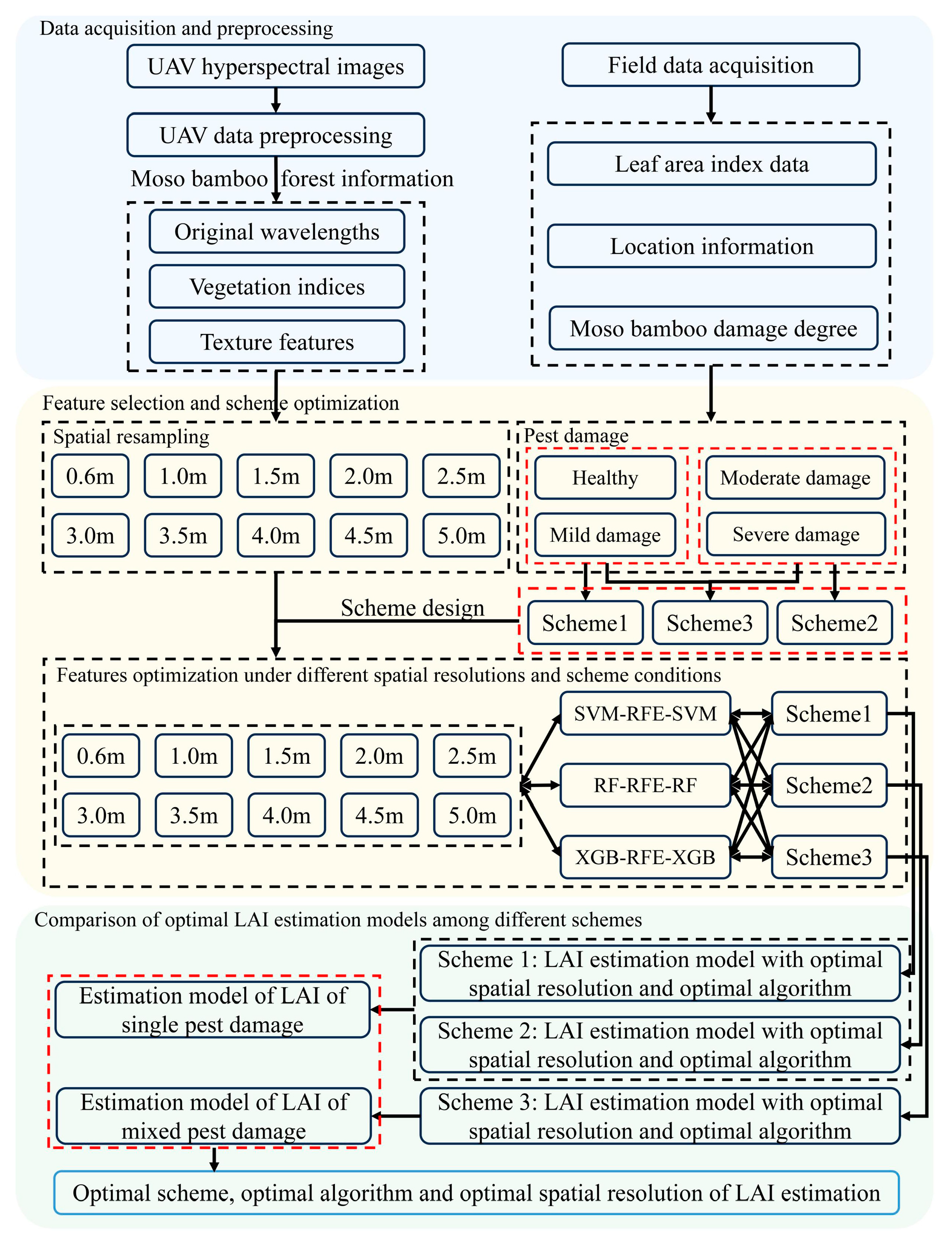
Multi-resolution remote sensing images: Considering the size of the bamboo canopy, a spatial scale that is too small may not cover the entire canopy, whereas one that is too large may include other objects. Therefore, a spatial scale interval of 0.5 m was chosen for resampling the hyperspectral data. The range of 0.6 to 5.0 m effectively addresses these concerns. Thus, in this study, the acquired 0.3 × 0.3 m UAV hyperspectral images were resampled into ten low spatial resolution images with resolutions of 0.6 m, 1 m, 1.5 m, 2 m, 2.5 m, 3 m, 3.5 m, 4 m, 4.5 m, and 5 m to investigate the effects of images with different spatial resolutions on LAI inversion. The resampling process utilized bilinear interpolation, calculating the value of each pixel by averaging the values of surrounding pixels.

(2)

Red edge parameter: This parameter serves as an indicator of plant health and is commonly used for detecting diseases and insect infestations in forests. The red edge index calculation formula selected for this study is provided in the following table (

Table 2. Calculation formula of red edge parameters and vegetation index.

Spectral Indices	Calculation Formula
Carotenoid Reflectance Index, CRI	$\mathrm{C}\mathrm{R}\mathrm{I}=1/{\rho }_{510}-1/{\rho }_{550}$
Enhanced Vegetation Index, EVI2	$\mathrm{E}\mathrm{V}\mathrm{I}2=2.5\times ({\rho }_{800}-{\rho }_{680})/({\rho }_{800}+2.4{\rho }_{680}+1)$
Gitelson-Merzlyak Index, GMI	$\mathrm{G}\mathrm{M}\mathrm{I}={\rho }_{750}/{\rho }_{700}$
Modified Red Edge Normalized Vegetation Index 705, mNDVI705	${\mathrm{mNDVI}}_{705}=({\rho }_{750}-{\rho }_{705})/({\rho }_{750}+{\rho }_{705}-2{\rho }_{445})$
Modified Red Edge Simple Ratio Index 705, mSR705	${\mathrm{mSR}}_{705}=({\rho }_{750}-{\rho }_{445})/({\rho }_{705}-{\rho }_{445})$
Normalized Difference Vegetation Index, NDVI	$\mathrm{N}\mathrm{D}\mathrm{V}\mathrm{I}=({\rho }_{800}-{\rho }_{680})/({\rho }_{800}+{\rho }_{680})$
Normalized Difference Vegetation Index 831, NDVI831	$\mathrm{N}\mathrm{D}\mathrm{V}{\mathrm{I}}_{831}=({\rho }_{831}-{\rho }_{667})/({\rho }_{831}+{\rho }_{667})$
Red Edge Normalized Difference Vegetation Index 705, NDVI705	$\mathrm{N}\mathrm{DV}{\mathrm{I}}_{705}=({\rho }_{750}-{\rho }_{705})/({\rho }_{750}+{\rho }_{705})$
Normalized Pigment Chlorophyll Index, NPCI	$\mathrm{N}\mathrm{P}\mathrm{C}\mathrm{I}=({\rho }_{680}-{\rho }_{430})/({\rho }_{680}+{\rho }_{430})$
Photochemical Reflectance Index, PRI	$\mathrm{P}\mathrm{R}\mathrm{I}=({\rho }_{680}-{\rho }_{430})/({\rho }_{680}+{\rho }_{430})$
Red Edge Difference Vegetation Index, REDVI	$\mathrm{R}\mathrm{E}\mathrm{D}\mathrm{V}\mathrm{I}={\rho }_{780}-{\rho }_{680}$
Red Edge Normalized Difference Vegetation Index, RENDVI	$\mathrm{R}\mathrm{E}\mathrm{N}\mathrm{D}\mathrm{V}\mathrm{I}=({\rho }_{780}-{\rho }_{680})/({\rho }_{780}+{\rho }_{680})$
Red Edge Ratio Index, RERVI	$\mathrm{R}\mathrm{E}\mathrm{R}\mathrm{V}\mathrm{I}={\rho }_{780}/{\rho }_{680}$
Ratio Vegetation Index, RVI	$\mathrm{R}\mathrm{V}\mathrm{I}={\rho }_{800}/{\rho }_{680}$
Soil-Adjusted Vegetation Index, SAVI	$\mathrm{S}\mathrm{A}\mathrm{V}\mathrm{I}=1.5\times ({\rho }_{800}-{\rho }_{680})/({\rho }_{800}-{\rho }_{680}+0.5)$
Structure Insensitive Pigment Index, SIPI	$\mathrm{S}\mathrm{I}\mathrm{P}\mathrm{I}=({\rho }_{800}-{\rho }_{445})/({\rho }_{800}-{\rho }_{680})$
Simple Ratio Pigment Index, SRPI	$\mathrm{S}\mathrm{R}\mathrm{P}\mathrm{I}={\rho }_{430}/{\rho }_{680}$
Transformed Chlorophyll Uptake Rate Index, TCARI	$\mathrm{T}\mathrm{C}\mathrm{A}\mathrm{R}\mathrm{I}=3\left[\left({\rho }_{700}-{\rho }_{670}\right)-0.2\left({\rho }_{700}-{\rho }_{550}\right)\left({\rho }_{700}/{\rho }_{550}\right)\right]$
Vogelmann Red Edge Index 1, VOG1	$\mathrm{V}\mathrm{O}{\mathrm{G}}_1={\rho }_{740}/{\rho }_{720}$
Vogelmann Red Edge Index 2, VOG2	$\mathrm{V}\mathrm{OG}2=({\rho }_{734}-{\rho }_{747})/({\rho }_{715}+{\rho }_{726})$
Vogelmann Red Edge Index 3, VOG3	$\mathrm{V}\mathrm{OG}3=({\rho }_{724}-{\rho }_{747})/({\rho }_{715}+{\rho }_{720})$
Water Band Index, WBI	$\mathrm{W}\mathrm{B}\mathrm{I}={\rho }_{900}/{\rho }_{970}$
Chlorophyll Absorption Ratio Index, CARI	$\begin{array}{l}\mathrm{C}\mathrm{A}\mathrm{R}\mathrm{I}=\left({\rho }_{700}/{\rho }_{670}\right)\left(\mathrm{a}{\rho }_{670}+{\rho }_{670}+\mathrm{b}\right)/\left(\sqrt{{\mathrm{a}}^2+1}\right),\\ \mathrm{a}={\displaystyle \frac{{\rho }_{700}-{\rho }_{550}}{150}},\mathrm{b}={\rho }_{550}-550\mathrm{a}\end{array}$
RE Band Chlorophyll Index, CIrededge	$\mathrm{C}\mathrm{I}\mathrm{r}\mathrm{e}\mathrm{d}\mathrm{e}\mathrm{d}\mathrm{g}=({\rho }_{750}-{\rho }_{800})/({\rho }_{695}-{\rho }_{740})-1$

${\rho }_{\mathrm{X}}$ is the original reflectance of band number X.

).

(3)

Spectral indices: There are numerous types of vegetation indices, and the infestation of P. phyllostachysae in bamboo stands exhibits a strong correlation with leaf water content and chlorophyll levels. Based on a review of previous studies, we selected the following vegetation indices to characterize the infestation (Table 2).

(4)

Texture features: Texture features are another category of indicators considered in remote sensing models, as they can reveal the spatial relationships between pixels and between individual pixels and the entire image. However, due to the large number of spectral bands in hyperspectral imagery, extracting texture features directly from the original hyperspectral bands is impractical and requires a significant amount of work. Therefore, dimensionality reduction is necessary. In this study, principal component analysis (PCA) was performed on raw hyperspectral images using ENVI 5.3 software to achieve dimensionality reduction. Following PCA processing, texture feature was extracted by calculating eight GLCM (Gray-Level Co-occurrence Matrix) parameters from the first principal component through the analytical modules of ENVI. The extracted texture features included mean, variance, homogeneity, contrast, dissimilarity, entropy, second moment, and correlation. The calculation formulas for the texture features selected are presented in

Table 3. Calculation formulas of texture features.

Texture Features	Calculation Formula
Mean	${\displaystyle \sum _{i=1}^n{\displaystyle \sum _{j=1}^{n}iP(i,j)}}$
Variance	${\displaystyle \sum _{i=1}^n{\displaystyle \sum _{j=1}^n{(i-\mu )}^{2}P}}(i,j)$
Homogeneity	${\displaystyle \sum _{i=1}^n{\displaystyle \sum _{j=1}^{n}P(i,j)/[1+{(i-j)}^2]}}$
Contrast	${\displaystyle \sum _{i=1}^n{\displaystyle \sum _{j=1}^{n}P(i,j)\times {(i-j)}^2}}$
Dissimilarity	${\displaystyle \sum _{i=1}^n{\displaystyle \sum _{j=1}^n\left|i-j\right|P(i,j)}}$
Entropy	${\displaystyle \sum _{i=1}^n{\displaystyle \sum _{j=1}^{n}P(i,j)\times \ln P(i-j)}}$
Second Moment	${\displaystyle \sum _{i=1}^n{\displaystyle \sum _{j=1}^{n}P{(i,j)}^2}}$
Correlation	$[{\displaystyle \sum _{i=1}^n{\displaystyle \sum _{j=1}^{n}P(i,j)\times (i-n)}}\times (j-n)]/({\sqrt{(i-n)}}^2\times {\sqrt{(j-n)}}^2)$

n is the maximum value of the pixel value, P(i,j) is the element of row i and column j in the joint grayscale matrix, and μ is the mean value of P(i,j).

.

(5)

Feature and model selection and optimization: Using SVM, RF, and XGBoost combined with the RFE algorithm, corresponding features were selected, and LAI estimation models were established for each scheme.

(6)

Model comparison across different schemes: By comparing the performance of the three schemes under different algorithms and spatial resolutions, the optimal estimation model for each scheme was selected. Additionally, the differences between the single pest level LAI estimation models (built from Scheme 1 and Scheme 2) and the mixed pest level LAI estimation model (built from Scheme 3) were analyzed.

2.3. Methods

2.3.1. Support Vector Machine

SVM, which constructs an optimal separating hyperplane as its fundamental concept, is a machine learning algorithm grounded in statistical theory [36]. Its core idea involves using kernel functions to nonlinearly map data into a high-dimensional feature space, constructing an optimal classification hyperplane with low VC dimensions (penalty parameter C; polynomial kernel parameter V) while comprehensively considering empirical risk and confidence intervals, following the principle of structural risk minimization (SRM) to determine the decision function.

2.3.2. Random Forest

RF is a machine learning algorithm that consists of multiple decision trees [37]. It begins by selecting training samples using a random bootstrap sampling strategy and then constructs a classification tree for each training sample set using the CART algorithm. At each node of the tree, the optimal feature is determined based on the Gini coefficient from a random subset of Mtry features selected from all available features. This process of sampling and tree construction is repeated to ultimately establish a random forest composed of multiple decision trees. During the classification phase, each decision tree independently predicts the class of new samples, and the final result is determined by aggregating the predictions of all decision trees using a majority voting principle.

2.3.3. Extreme Gradient Boosting

XGBoost is an ensemble learning algorithm based on boosting trees, designed to study gradient boosting decision tree algorithms [38]. Built upon Gradient Boosting Decision Tree (GBDT), this algorithm represents an improved Boosting model with advantages such as high computational efficiency and strong scalability. At its core, XGBoost involves the continuous growth of trees, constructing prediction trees through feature learning. Each additional tree essentially learns a new function to fit the residuals, with the final prediction being the sum of the predictions from all trees. The algorithm is capable of addressing both classification and regression tasks, excelling at capturing complex interactions and nonlinear relationships between variables. It features built-in cross-validation for optimal parameter selection, enhancing model performance, and incorporates parallel and approximate computations to accelerate processing. Additionally, XGBoost introduces regularization terms to effectively control model complexity, improve generalization capability, and demonstrate robustness to outliers.

2.3.4. Recursive Feature Elimination

Hyperspectral data comprise a large number of spectral bands and a wealth of derived indices. This study proposes to adopt machine learning algorithms combined with RFE to select typical differential indices, with the aim of deeply analyzing the spectral information of bamboo forests from UAV hyperspectral data and effectively extracting spectral response features. RFE, as a greedy algorithm, operates by iteratively constructing models to select the optimal subset of features for regression [39]. The algorithm identifies the most or least significant features based on their coefficients, removes them, and repeats the process on the remaining features until all features have been evaluated. The order of feature elimination determines their ranking. To further determine the optimal number of features significantly related to the LAI, this study employs RFE combined with five-fold cross-validation to select the best feature set.

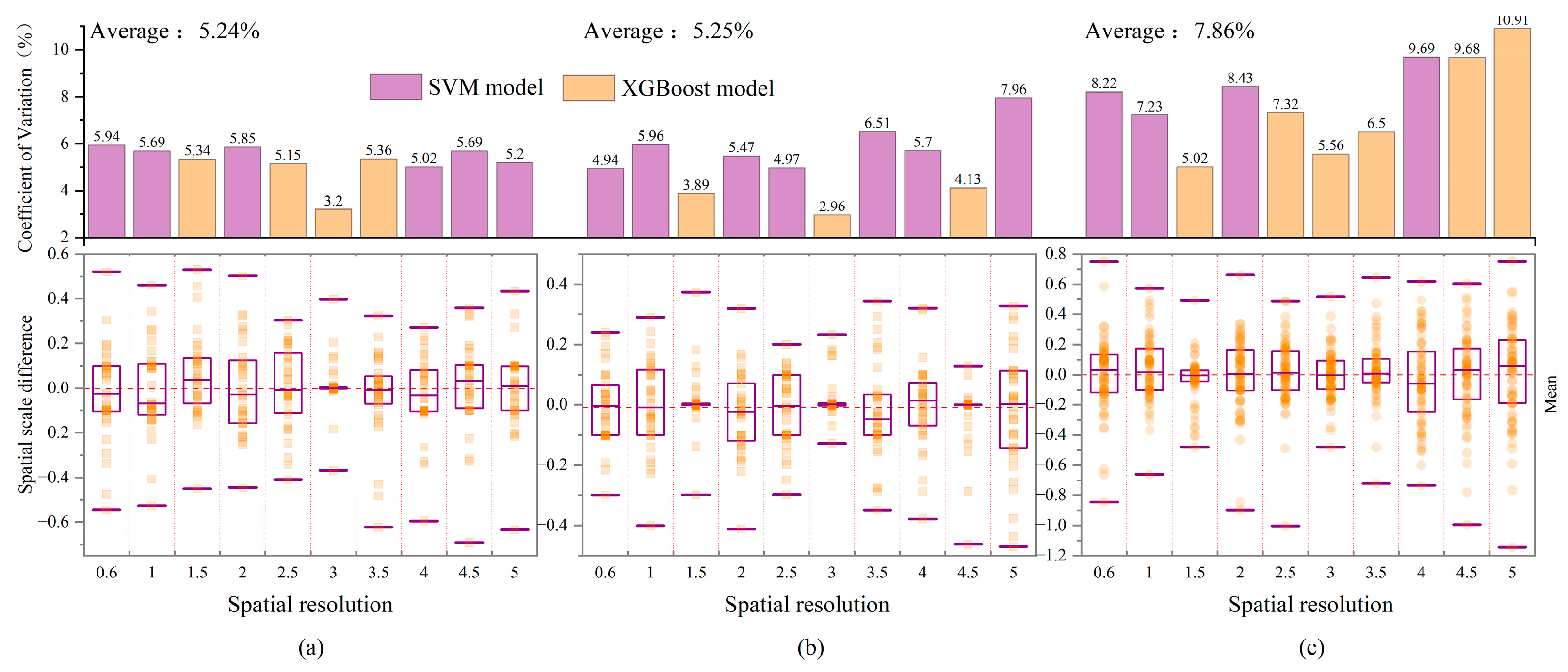
2.3.5. Coefficient of Variation

The coefficient of variation (CV) provides a metric to compare the variability across different datasets or variables [40]. A higher coefficient of variation indicates a greater relative variability between datasets or variables, while a lower value suggests less variability. This method is advantageous because it allows for the comparison of variability without being influenced by differences in the magnitude of the data. Therefore, when analyzing differences in LAI across different spatial scales, the coefficient of variation can be used to quantify the relative variability between LAI values derived from different spatial resolutions and ground-measured values. This enables the study of spatial scale effects. The coefficient of variation is calculated as follows:

$$\mathrm{cv}={\displaystyle \frac{\sqrt{\frac{1}{n}{\displaystyle \sum _{i=1}^{\mathrm{n}}{(x_{i,j}-x_i)}^2}}}{\overline{x_i}}}\times 100\%$$

(1)

where j represents the spatial resolution, X_i is the measured value, X_i,j is the model-predicted value corresponding to X_i at spatial resolution j, $x_{i,j}-x_i$ is the difference between the model-predicted value and the measured value, and $\overline{x_i}$ is the mean of the measured values.

3. Results

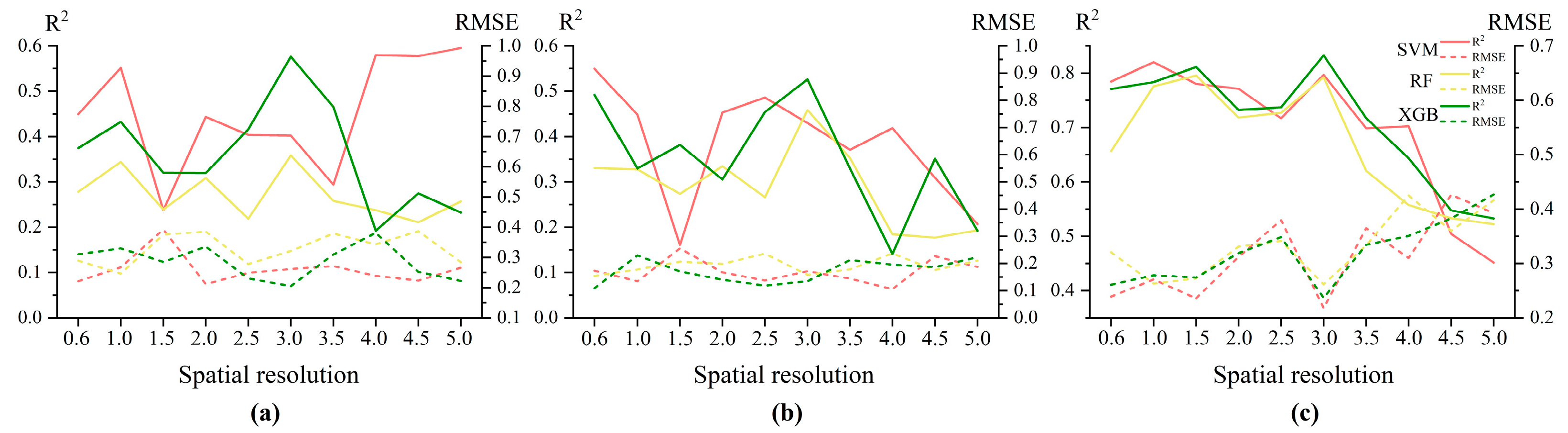
3.1. Comparison of Different Spatial Resolution Estimation Models

Given the large number of spectral features, this study employs the RFE algorithm in combination with RF, SVM, and XGBoost to select typical differential indices. In both the RFE feature selection and model-building processes, parameter tuning is essential for optimizing model performance. This typically involves using grid search and cross-validation for hyperparameter optimization. Combining grid search with cross-validation allows for the evaluation of each hyperparameter combination to find the best-suited configuration for the dataset. For dataset partitioning, a 7:3 strategy was employed, with 7 for the training set and 3 for the test set. During RFE feature selection, the feature quantity and corresponding factors at the highest OA were chosen for modeling, which can significantly enhance model accuracy.

For the three schemes, the study performs an importance ranking of 332 feature factors (including 300 original bands, 24 spectral indices, and 8 texture features) across 10 different spatial scales. This process aims to determine the number of feature parameters significantly correlated with the LAI and their corresponding feature factors, reducing data redundancy between different types of factors. We then constructed machine learning models, enhancing their predictive capability and accuracy. To identify the optimal models for estimating bamboo LAI under different spatial resolutions, the study evaluates key performance metrics, including the R² and the root mean square error (RMSE), for the LAI estimation models.

3.1.1. Comparison of Different Spatial Resolution Estimation Models Based on SVM Regression Algorithm

Based on the previous support vector machine-recursive feature elimination (SVM-RFE) feature selection results, the corresponding SVM LAI estimation model was established. The precision of the model, constructed using the support vector machine regression algorithm, is as follows:

According to the results shown in

Table 4. Accuracy of SVM regression model.

Spatial Resolution	Scheme 1		Scheme 2		Scheme 3
	R2	RMSE	R2	RMSE	R2	RMSE
0.6 m	0.4494	0.2211	0.5499	0.1731	0.7843	0.2391
1 m	0.5514	0.2671	0.4481	0.1347	0.8201	0.2706
1.5 m	0.2373	0.3926	0.1607	0.2553	0.7801	0.2359
2 m	0.4434	0.2116	0.4529	0.1671	0.7712	0.3119
2.5 m	0.4036	0.2487	0.4859	0.1373	0.7169	0.3797
3 m	0.4023	0.2619	0.4297	0.1712	0.7969	0.2178
3.5 m	0.2937	0.2711	0.3708	0.1439	0.6985	0.3648
4 m	0.5801	0.2388	0.4185	0.1056	0.7024	0.3098
4.5 m	0.5774	0.2231	0.3091	0.2268	0.5043	0.4263
5 m	0.5957	0.2656	0.2068	0.1873	0.4515	0.3925

The bold content is the optimal precision in the scheme.

, it can be observed that the three schemes exhibit varying performances in the support vector machine regression model, with each scheme having its optimal spatial resolution for LAI inversion. In terms of the overall performance of R², Scheme 1 outperforms Scheme 2, indicating that the LAI inversion for healthy and mildly damaged bamboo forests is more excellent than that for moderately and severely damaged forests. However, considering the overall performance of the RMSE, Scheme 2 surpasses Scheme 1, suggesting that the LAI inversion errors for moderately and severely damaged bamboo forests are lower than those for healthy and mildly damaged forests. This indicates that the support vector machine regression algorithm does not show a significant advantage in the LAI inversion effects across different pest damage levels of bamboo forests. Scheme 3 demonstrates good precision in LAI inversion for bamboo forests at spatial resolutions of 0.6 to 4 m, with R² consistently exceeding 0.69. However, at spatial resolutions of 4.5 to 5 m, the R² significantly decreases with increasing resolution, accompanied by a substantial rise in RMSE.

In Scheme 1, the spatial resolution with the highest R² is 5 m, followed by 4 m, 4.5 m, and 1 m. However, RMSE is optimal at a spatial resolution of 2 m. Therefore, a comprehensive consideration of both the R² and RMSE is necessary. The spatial resolution that achieves a relatively high R² while minimizing the RMSE is selected as the optimal spatial scale. Thus, 4.5 m was chosen as the optimal spatial resolution for Scheme 1 using the support vector machine regression algorithm. Similarly, in Scheme 2, the spatial resolution with the highest R² is 0.6 m, followed by 2.5 m, 2 m, and 1 m. The RMSE is lowest at a spatial resolution of 4 m, followed by 1 m and 2.5 m. Therefore, 2.5 m was selected as the optimal spatial resolution for Scheme 2 using the support vector machine regression algorithm. For Scheme 3, the spatial resolution with the highest R² is 1 m, followed by 3 m, 0.6 m, and 1.5 m. The RMSE is lowest at a spatial resolution of 3 m, followed by 1.5 m and 0.6 m. Therefore, 3 m was chosen as the optimal spatial resolution for Scheme 3 using the support vector machine regression algorithm.

3.1.2. Comparison of Different Spatial Resolution Estimation Models Based on RF Regression Algorithm

Based on the previous random forest-recursive feature elimination (RF-RFE) feature selection results, the corresponding RF LAI estimation model was established. The precision of the model, constructed using the random forest regression algorithm, is as follows:

According to the results shown in

Table 5. Accuracy of RF regression model.

Spatial Resolution	Scheme 1		Scheme 2		Scheme 3
	R2	RMSE	R2	RMSE	R2	RMSE
0.6 m	0.2781	0.2891	0.3306	0.1543	0.6564	0.3207
1 m	0.3441	0.2465	0.3277	0.1777	0.7756	0.2628
1.5 m	0.2391	0.3756	0.2736	0.2065	0.7954	0.2727
2 m	0.3085	0.3853	0.3345	0.1986	0.7183	0.3309
2.5 m	0.2188	0.2776	0.2662	0.2363	0.7269	0.3416
3 m	0.3585	0.3216	0.4586	0.1581	0.7923	0.2617
3.5 m	0.2579	0.3788	0.3525	0.1783	0.6203	0.3334
4 m	0.2375	0.3435	0.1842	0.2364	0.5574	0.4251
4.5 m	0.2109	0.3869	0.1769	0.1761	0.5331	0.3601
5 m	0.2569	0.2841	0.1933	0.2101	0.5221	0.4162

The bold content is the optimal precision in the scheme.

, it can be observed that the three schemes exhibit varying performances in the random forest regression model, with each scheme having its optimal spatial resolution for LAI inversion. From the overall perspective of R², Scheme 2 performs better than Scheme 1, indicating that the LAI inversion effects for moderately and severely damaged bamboo forests are superior to those for healthy and mildly damaged forests. Additionally, from the overall perspective of RMSE, Scheme 2 also outperforms Scheme 1, meaning that the inversion errors for the LAI of moderately and severely damaged bamboo forests are lower than those for healthy and mildly damaged forests. This demonstrates that the random forest regression algorithm significantly improves the LAI inversion performance for Scheme 2 compared to Scheme 1. Scheme 3 achieves good accuracy in LAI inversion for bamboo forests across spatial resolutions of 0.6–3.5 m, with the R² values all exceeding 0.62. However, at spatial resolutions of 4–5 m, the R² decreases to varying degrees as the spatial resolution increases, and the RMSE also increases accordingly.

In Scheme 1, the spatial resolution with the highest R² is 3 m, followed by 1 m and 2 m. However, the RMSE is best when the spatial resolution is 1 m. Therefore, it is necessary to consider both the R² and the RMSE comprehensively. While maintaining a relatively high R², the RMSE should be minimized. Thus, 1 m was selected as the optimal spatial resolution for Scheme 1 under the random forest regression algorithm. Similarly, in Scheme 2, the spatial resolution with the highest R² is 3 m, followed by 3.5 m, 2 m, and 0.6 m. The RMSE is lowest at 3 m, followed by 4.5 m, 1 m, and 3.5 m. Therefore, 3 m was chosen as the optimal spatial resolution for Scheme 2 under the random forest regression algorithm. For Scheme 3, the spatial resolution with the highest R² is 1.5 m, followed by 3 m, 1 m, and 2.5 m. The RMSE is lowest at 3 m, followed by 1 m and 1.5 m. Hence, 3 m was selected as the optimal spatial resolution for Scheme 3 under the random forest regression algorithm.

3.1.3. Comparison of Different Spatial Resolution Estimation Models Based on XGBoost Regression Algorithm

Based on the previous extreme gradient boosting-recursive feature elimination (XGB-RFE) feature selection results, the corresponding XGBoost LAI estimation model was established. The precision of the model, constructed using the extreme gradient boosting tree regression algorithm, is as follows:

According to the results shown in

Table 6. Accuracy of XGBoost regression model.

Spatial Resolution	Scheme 1		Scheme 2		Scheme 3
	R2	RMSE	R2	RMSE	R2	RMSE
0.6 m	0.3746	0.3104	0.4923	0.1086	0.7708	0.2608
1 m	0.4323	0.3297	0.3295	0.2297	0.7835	0.2782
1.5 m	0.3199	0.2851	0.3815	0.1702	0.8113	0.2741
2 m	0.3194	0.3358	0.3053	0.1404	0.7321	0.3189
2.5 m	0.4159	0.2302	0.4541	0.1186	0.7371	0.3484
3 m	0.5764	0.2048	0.5261	0.1346	0.8326	0.2366
3.5 m	0.4654	0.3097	0.3294	0.2125	0.7172	0.3344
4 m	0.1922	0.3811	0.1412	0.1957	0.6434	0.3506
4.5 m	0.2745	0.252	0.3512	0.1864	0.5476	0.3827
5 m	0.2324	0.2218	0.1918	0.2229	0.5328	0.4268

The bold content is the optimal precision in the scheme.

, it can be observed that the three schemes exhibit varying performances in the extreme gradient boosting tree regression model, with each scheme having its optimal spatial resolution for LAI inversion. From the overall perspective of R², Scheme 1 performs better than Scheme 2, indicating that the LAI inversion effects for healthy and mildly damaged bamboo forests are superior to those for moderately and severely damaged forests. However, from the overall perspective of RMSE, Scheme 2 outperforms Scheme 1, meaning that the inversion errors for the LAI of moderately and severely damaged bamboo forests are lower than those for healthy and mildly damaged forests. This suggests that the extreme gradient boosting tree regression algorithm does not show a significant advantage in improving the LAI inversion effects for bamboo forests with different pest damage levels. Scheme 3 achieves good precision in LAI inversion for bamboo forests across spatial resolutions of 0.6–3.5 m, with the R² values all exceeding 0.71. However, at spatial resolutions of 4–5 m, the R² decreases significantly as the spatial resolution increases, and the RMSE also increases substantially with rising spatial resolution.

In Scheme 1, the spatial resolution with the highest determination coefficient is 3 m, followed by 3.5 m and 1 m. The spatial resolution with the lowest RMSE is 3 m, followed by 5 m and 2.5 m. Therefore, 3 m was selected as the optimal spatial resolution for Scheme 1 under the extreme gradient boosting tree regression algorithm. Similarly, in Scheme 2, the spatial resolution with the highest determination coefficient is 3 m, followed by 0.6 m and 2.5 m. The spatial resolution with the lowest RMSE is 0.6 m, followed by 2.5 m, 3 m, and 2 m. Thus, considering comprehensively, 3 m was chosen as the optimal spatial resolution for Scheme 2 under the extreme gradient boosting tree regression algorithm. For Scheme 3, the spatial resolution with the highest determination coefficient is 3 m, followed by 1.5 m, 1 m, and 0.6 m. The spatial resolution with the lowest RMSE is 3 m, followed by 0.6 m, 1.5 m, and 1 m. Hence, 3 m was selected as the optimal spatial resolution for Scheme 3 under the extreme gradient boosting tree regression algorithm.

3.1.4. Comparison of Different Algorithms Under the Optimal Spatial Resolution Estimation Model

Through the comparison of LAI inversion model performance established by three machine learning algorithms, it can be observed that different machine learning algorithms exhibit varying effects on the inversion of bamboo forest LAI (Figure 3). In the study of LAI inversion for Scheme 1, 4.5 m, 1 m, and 3 m were selected as the optimal spatial resolutions for SVM, RF, and XGBoost, respectively. However, when comparing the inversion performance of different regression models, it was found that SVM > XGBoost > RF. The SVM algorithm demonstrated a superior inversion effect for Scheme 1, maintaining high R² and low RMSE across both low and high spatial resolutions. In contrast, the XGBoost algorithm only achieved high R² and low RMSE at moderate spatial resolutions (2.5–3.5 m), and the RF algorithm showed no significant advantages in Scheme 1’s LAI inversion. Considering the inversion performance of both SVM and XGBoost algorithms comprehensively, it was noted that although SVM slightly outperformed XGBoost in single pest-level models, its model stability was inferior to that of XGBoost. Therefore, the 3 m spatial resolution, which exhibited comparable R² values and the lowest RMSE in the XGBoost algorithm, was ultimately selected as the optimal LAI inversion scheme for Scheme 1.

In the study of LAI inversion for Scheme 2, the optimal spatial resolutions of 2.5 m, 3 m, and 3 m were selected for SVM, RF, and XGBoost, respectively. However, when comparing the inversion performance of different regression models, a similar pattern emerged: SVM > XGBoost > RF. The SVM algorithm also demonstrated a strong inversion performance for Scheme 2, maintaining high R² values across multiple spatial resolutions. In contrast, the XGBoost algorithm only achieved high R² values and low RMSE under specific spatial resolutions, while the RF algorithm showed no significant advantages in Scheme 2’s LAI inversion. When comprehensively evaluating the inversion performance of both the SVM and XGBoost algorithms, it was observed that although SVM slightly outperformed XGBoost in single pest-level models, the stability of SVM models remained inferior to that of XGBoost. Therefore, the 3 m spatial resolution, which exhibited the highest R² and the lowest RMSE in the XGBoost algorithm, was ultimately selected as the optimal LAI inversion scheme for Scheme 2.

In the study of LAI inversion for Scheme 3, the optimal spatial resolutions of 3 m, 3 m, and 3 m were selected for SVM, RF, and XGBoost, respectively. However, when comparing the inversion performance of different regression models, it was observed that XGBoost > SVM > RF. The XGBoost algorithm demonstrated a strong inversion performance for Scheme 3, maintaining high R² values across multiple spatial resolutions. In contrast, the SVM algorithm only achieved high R² values and low RMSE under specific spatial resolutions, while the RF algorithm, again, showed no significant advantages in Scheme 3’s LAI inversion. All three machine learning methods exhibited identical trends in inversion performance, achieving optimal results at the 3 m spatial resolution. When comprehensively evaluating the inversion performance of both the SVM and XGBoost algorithms, it was noted that in mixed pest-level models, XGBoost slightly outperformed SVM. Therefore, the 3 m spatial resolution, which exhibited the highest R² values in the XGBoost algorithm, was ultimately selected as the optimal LAI inversion scheme for Scheme 3.

3.2. Spatial Scale Effect Difference of Leaf Area Index Under Different Schemes

Through a comparative analysis of LAI estimation models at different spatial resolutions across the three schemes, it was observed that optimal algorithm and model performance vary under different spatial resolutions. To further compare the differences in LAI model inversion due to varying spatial resolutions, the coefficient of variation method was applied. This method compares the inversion results of optimal machine learning models at different spatial resolutions with measured data values, enabling a quantitative comparison and evaluation of the impact of spatial resolution on LAI. The impact of spatial resolution on LAI, as reflected in the magnitude of the coefficient of variation and differences in spatial scale across various resolutions (as shown in Figure 4), revealed that the average coefficient of variation for Scheme 1 and Scheme 2 was similar, the average coefficient of variation for Scheme 3 was lower than the sum of those for Scheme 1 and Scheme 2. Additionally, Scheme 3 exhibited slightly greater differences in spatial scale compared to Schemes 1 and 2.

The coefficient of variation in Scheme 1 remained below 6%, with a mean variation of 5.24%. Notably, the LAI exhibited only 3.2% variation at 3 m spatial resolution, while other resolutions showed variations in the range of 5–6%. Minimal scale discrepancies were observed specifically at 3 m resolution. Scheme 2 demonstrated greater variability, with coefficients in the range of 2.96–7.96%, though maintaining comparable mean variation (5.25%) to Scheme 1. The LAI variation reached its minimum (2.96%) at 3 m resolution, followed by 3.89% at 1.5 m resolution, with other resolutions showing 4–8% fluctuations. Relatively small-scale variations were identified at 3 m, 1.5 m, and 4.5 m resolutions. Scheme 3 displayed the widest variation range (5–11%) with a mean value of 7.86%. Specifically, the LAI changes by only 5.02% at a spatial resolution of 1.5 m, followed by a 5.56% change at 3 m. For other spatial resolutions, the LAI changes in the range between 6% and 11%. The smallest differences in spatial scale are observed at 1.5 m and 3 m. Further analysis of spatial scale effects demonstrates the feasibility of a 3 m resolution as the optimal spatial resolution for LAI estimation, as it exhibits the smaller spatial scale differences across all three schemes, thereby providing superior inversion capability in LAI studies.

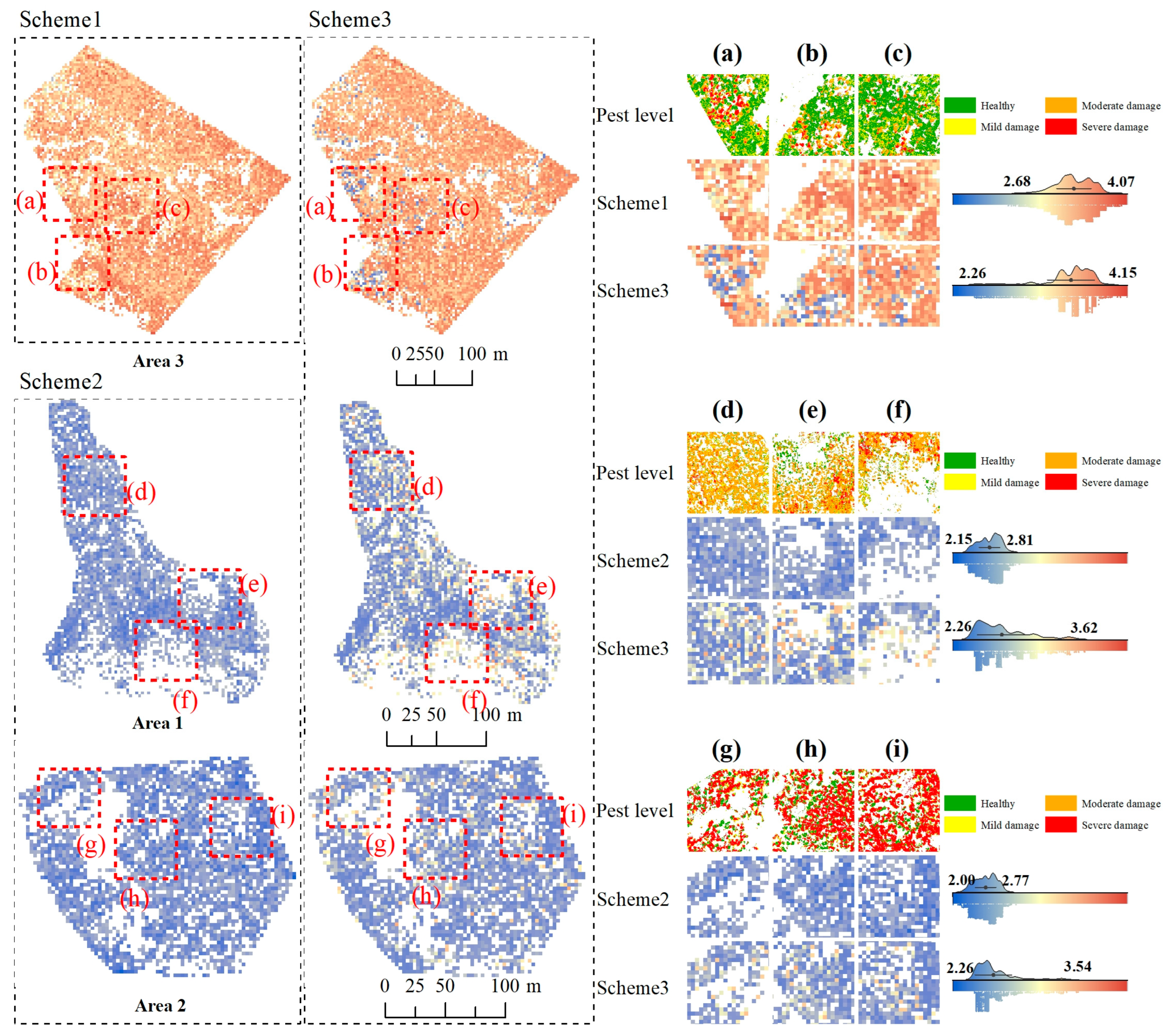
3.3. Remote Sensing Inversion of Leaf Area Index Using the Optimal Spatial Resolution and Algorithm

Based on the accuracy performance of the three machine learning algorithms under different spatial resolution scenarios across the three schemes, it can be observed that the SVM algorithm demonstrates the best model performance in estimating the LAI for single pest damage levels in bamboo forests, slightly outperforming the XGBoost algorithm. Both algorithms consistently achieve the best inversion effects across different spatial resolution scenarios. However, when studying the overall impact of mixed pest damage levels on bamboo forests, the XGBoost algorithm delivers superior inversion performance. Based on the aforementioned analysis, the XGBoost algorithm with a 3 m spatial resolution was selected as the optimal algorithm and spatial scale for the three schemes. Therefore, this algorithm was applied to 3 m spatial resolution UAV imagery for LAI remote sensing inversion, aiming to achieve the optimal LAI inversion results.

As shown in Figure 5, the LAI of bamboo forests in the study area primarily ranges from 2.0 to 4.15, with Area 3 generally exhibiting higher LAI values compared to Areas 1 and 2. Scheme 1’s LAI primarily ranges from 2.68 to 4.07, demonstrating better inversion performance for healthy and mildly damaged bamboo forests. A relatively clear distinction in LAI is observed between healthy and mildly damaged bamboo forests. Scheme 2’s LAI primarily ranges from 2.00 to 2.81, with poorer inversion performance for moderately and severely damaged bamboo forests. A noticeable difference in LAI is observed between moderate and severe damage levels in Area 1, whereas no significant difference is found in Area 2, which has poor inversion performance. Scheme 3’s LAI primarily ranges from 2.26 to 4.15, demonstrating excellent inversion performance across all pest damage levels. Compared to the other two schemes, Scheme 3 shows a significant advantage in mixed damage level bamboo forests, effectively distinguishing and estimating the LAI of bamboo forests under different pest damage levels.

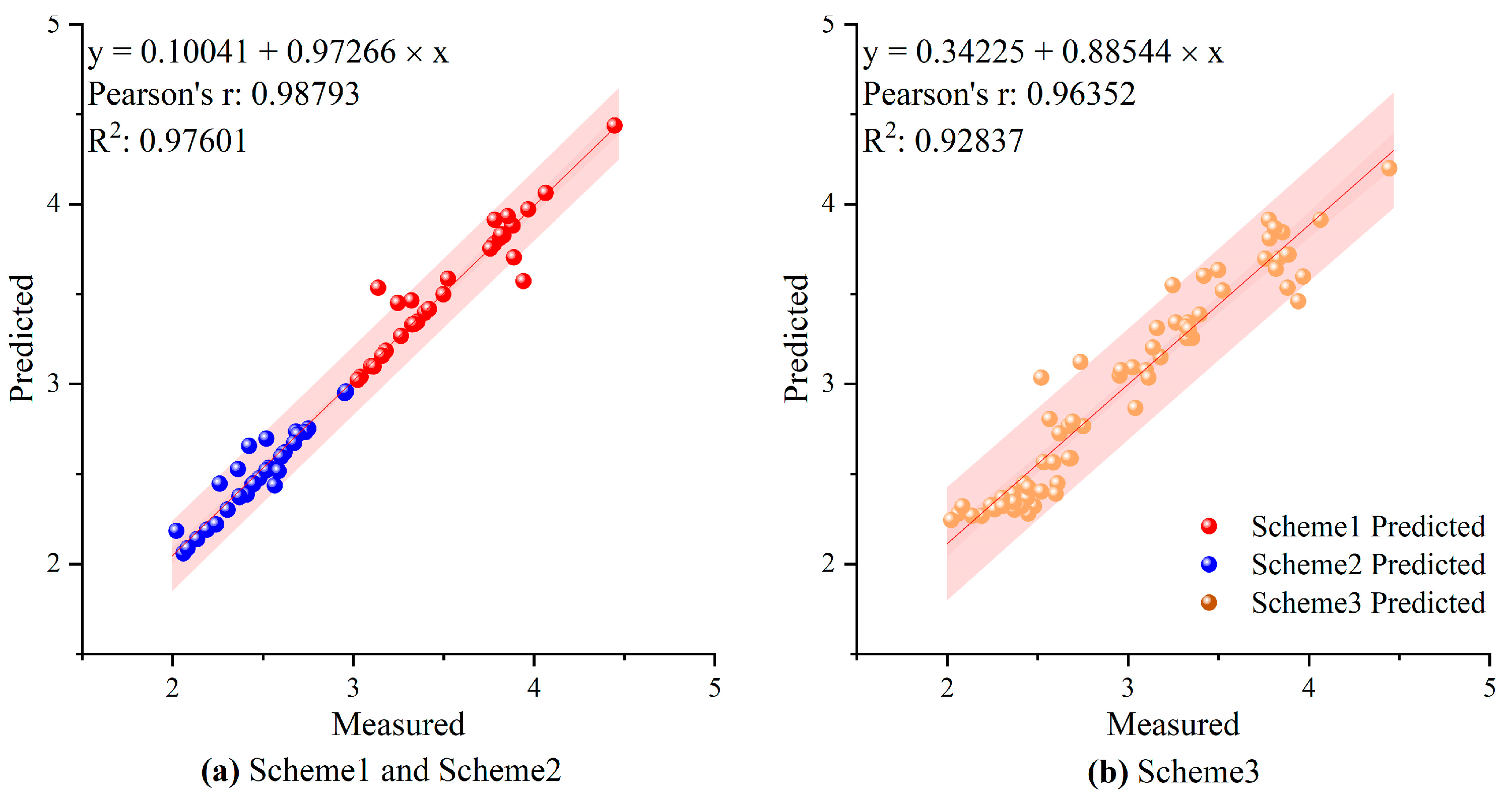
3.4. Comparison of Leaf Area Index Models Between Single Pest Damage Levels and Mixed Pest Damage Levels

From the above conclusions, we found that in actual inversion, the LAI model for mixed pest damage level bamboo forests has better inversion performance than the single pest damage level model. However, at the model level, it remains unclear whether Scheme 1 is superior or inferior to Schemes 2 and 3. By establishing LAI estimation models through the three schemes and using them to predict measured values, we can compare the model effects between mixed and single pest damage level models, effectively reflecting their respective advantages and disadvantages. As shown in Figure 6, the relationship between the predicted and measured values of the sampling points indicates that Schemes 1 and 2 achieved Pearson’s r and R² values of 0.9879 and 0.9760, respectively, while Scheme 3 achieved lower values of 0.9635 and 0.9283. Therefore, from the perspective of model performance on the measured dataset, single pest damage level LAI models demonstrate higher estimation accuracy compared to mixed pest damage level models.

4. Discussion

4.1. Effect of Bamboo Forest On-Year and Off-Year Phenomenon on Leaf Area Index

The growth of bamboo follows its own growth patterns, where it sprouts and grows into culms in one year and then sheds its leaves and renews its shoots the next year. Within the same bamboo forest, nearly all bamboo plants share the same phenological characteristics, resulting in synchronized growth phases of either sprouting and culm development or shoot replacement and leaf renewal, thereby forming bamboo stands with distinct phenological (on-year and off-year) conditions [16]. While on-year and off-year bamboo stands under pest stress exhibit similar physiological characteristics, their resistance to pests differs [41]. Consequently, the changes in LAI under pest stress may also vary between on-year and off-year stands. To develop appropriate LAI estimation models for on-year and off-year bamboo stands, further research is required to investigate the variations in LAI caused by pest damage in bamboo forests and to explore the underlying mechanisms by which pests affect on-year and off-year bamboo stands.

4.2. Applicability of Mixed Pest Damage Leaf Area Index Model and Single Pest Damage Model

In estimating the LAI of bamboo forests, this study approaches from the perspective of pest stress, investigating optimal algorithms, spatial resolutions, and inversion methods to establish estimation models for accurate LAI prediction. Considering pest stress is crucial, as the bamboo moth, a foliage-feeding pest, causes irreversible damage to the bamboo canopy, leading to sparse leaves and reduced LAI. Ignoring pest factors in LAI inversion inevitably reduces accuracy. As shown in the results, models considering pest levels have improved R² by 0.0477 and Pearson’s r by 0.0144 compared to those ignoring pest factors, demonstrating better performance. Although mixed pest-level models perform better overall, models accounting for pest levels excel in single pest-level inversions. Establishing optimal models for each pest level and merging results can yield superior performance compared to a single model for all pest levels.

Previous studies have already found that PROSAIL models based on different pest infestation levels outperform traditional PROSAIL models in terms of inversion performance [16]. Since LAI serves as an intermediate variable in the PROSAIL model, improving the accuracy of LAI inversion would necessarily lead to a significant enhancement in the overall performance of the PROSAIL model. This insight has guided the present study and led to the same conclusion. For plants other than bamboo forests, such as pine trees—the LAI of which decreases due to pine caterpillar damage—the methodology presented in this study could theoretically be applied to investigate LAI under pest stress. However, the actual inversion performance would require further exploration in future studies.

4.3. Influencing Factors of Spatial Scale Efficiency of Leaf Area Index

In UAV-based LAI inversion studies, research often focuses on homogeneous crops, using controlled variables to assess factors impacting LAI without considering the spatial resolution of UAV images [18]. In contrast, bamboo forest LAI inversion is significantly affected by spatial heterogeneity, resolution, and pest damage levels. Most models in this study perform best at a 3-m resolution, likely because Moso bamboo’s natural curvature creates a larger canopy projection, making pest differences more evident and reducing spatial heterogeneity’s impact at this scale. Additionally, the original spatial resolution of UAV images and image resampling may introduce LAI estimation errors. Future research could improve data collection by capturing images at different resolutions via varied UAV flight heights.

5. Conclusions

(1)

By comparing the performance of LAI estimation models and analyzing spatial scale effects across different spatial resolutions, the combination of the XGBoost algorithm and a 3 m spatial resolution was identified as the optimal choice for the three schemes.

(2)

The coefficient of variation method further confirmed the XGBoost algorithm’s excellent LAI inversion capability and the accuracy of the 3 m spatial resolution for LAI estimation.

(3)

All three schemes show good inversion performance. Compared with the mixed pest-level LAI model, the single pest-level LAI model has higher estimation accuracy and a clear advantage in homogeneous pest-level regions of Moso bamboo forests.

The findings of this study enhance the precision of LAI remote sensing inversion. This helps promptly identify pest sources and implement control measures to curb their spread. Consequently, it safeguards the health of bamboo forest ecosystems and ensures the efficient use of bamboo resources.

References

1. Watson, D.J. Comparative physiological studies on the growth of field crops: I. Variation in net assimilation rate and leaf area between species and varieties, and within and between years. Ann. Bot. Bot. 1947, 11, 41–76. [Google Scholar]
2. Wang, X.Q.; Ma, L.Y.; Jia, Z.K.; Xu, C.Y. Research and application advances in leaf area index (LAl). Chin. J. Ecol. 2005, 5, 537–541. [Google Scholar]
3. Wu, W.B.; Hong, T.S.; Wang, X.P.; Peng, W.X.; Li, Z.; Zhang, W.Z. Advance in ground-based LAl measurement methods. J. Huazhong Agric. Univ. 2007, 2, 270–275. [Google Scholar]
4. Yan, G.J.; Hu, R.H.; Luo, J.H.; Weiss, M.; Jiang, H.L.; Mu, X.H.; Xie, D.H.; Zhang, W.M. Review of indirect optical measurements of leaf area index: Recent advances, challenges, and perspectives. Agric. For. Meteorol. 2019, 265, 390–411. [Google Scholar]
5. Ziliani, M.G.; Altaf, M.U.; Aragon, B.; Houborg, R.; Franz, T.E.; Lu, Y.; Sheffield, J.; Hoteit, I.; McCabe, M.F. Early season prediction of within-field crop yield variability by assimilating CubeSat data into a crop model. Agric. For. Meteorol. 2022, 313, 108736. [Google Scholar]
6. Liu, S.B.; Jin, X.L.; Nie, C.W.; Wang, S.Y.; Yu, X.; Cheng, M.H.; Shao, M.C.; Wang, Z.X.; Tuohuti, N.; Bai, Y.; et al. Estimating leaf area index using unmanned aerial vehicle data: Shallow vs. deep machine learning algorithms. Plant Physiol. 2021, 187, 1551–1576. [Google Scholar]
7. Huang, H.; Huang, J.; Wu, Y.; Zhuo, W.; Song, J.; Li, X.; Li, L.; Su, W.; Ma, H.; Liang, S. The improved winter wheat yield estimation by assimilating GLASS LAI Into a crop growth model with the proposed Bayesian Posterior-based ensemble kalman filter. IEEE Trans. Geosci. Remote Sens. 2023, 61, 4401818. [Google Scholar]
8. Wang, Y.L.; Wang, J.; Cui, T. Inversion of leaf area index of Silage Corn based on PROSAIL model. Trans. Chin. Soc. Agric. Eng. 2024, 55, 205–213. [Google Scholar]
9. Chen, S.D.; Chen, Y.G.; Xu, X.J.; Liu, J.Y.; Guo, J.Z.; Hu, S.Y.; Lan, Y.B. Monitoring of corn leaf area index based on multispectral remote sensing of UAV. J. South China Agric. Univ. 2024, 45, 608–617. [Google Scholar]
10. Li, C.H.; Li, B.Y.; Mao, Z.W.; Li, L.F.; Yu, K.Y.; Liu, J.; Zhong, Q.L. Canopy hyperspectral modeling of leaf area index at different expansion stages of Phyllostachys edulis into cunninghamia lanceolata forest. Spectrosc. Spectr. Anal. 2024, 44, 2365–2371. [Google Scholar]
11. Bao, G.D.; Liu, T.; Zhang, Z.H.; Ren, Z.B.; Zhai, C.; Ding, M.M.; Jiang, X.F. Remote sensing inversion of effective leaf area index of four coniferous forest types and their spatial distribution rule in changbai mountain. Sci. Silvae Sin. 2024, 60, 127–138. [Google Scholar]
12. Gu, C.Y.; Du, H.Q.; Zhou, G.M.; Han, N.; Xu, X.J.; Zhao, X.; Sun, X.Y. Retrieval of leaf area index of moso bamboo forest with Landsat Thematic Mapper image based on PROSAIL canopy radiative transfer model. J. Appl. Ecol. 2013, 24, 2248–2256. [Google Scholar]
13. Yue, J.B.; Yang, H.; Yang, G.J.; Fu, Y.Y.; Wang, H.; Zhou, C.Q. Estimating vertically growing crop above-ground biomass based on UAV remote sensing. Comput. Electron. Agric. 2023, 205, 107627. [Google Scholar]
14. Zhang, J.J.; Cheng, T.; Guo, W.; Xu, X.; Qiao, H.B.; Xie, Y.M.; Ma, X.M. Leaf area index estimation model for UAV image hyperspectral data based on wavelength variable selection and machine learning methods. Plant Methods 2021, 17, 49. [Google Scholar] [PubMed]
15. Zhang, Y.; Yang, Y.; Zhang, Q.; Duan, R.; Liu, J.; Qin, Y.; Wang, X. Toward multi-stage phenotyping of soybean with multimodal UAV sensor data: A comparison of machine learning approaches for leaf area index estimation. Remote Sens. 2023, 15, 7. [Google Scholar]
16. Xu, Z.H.; He, A.Q.; Zhang, Y.W.; Hao, Z.B.; Li, Y.F.; Xiang, S.Y.; Li, B.; Chen, L.Y.; Yu, H.; Shen, W.L.; et al. Retrieving chlorophyll content and equivalent water thickness of Moso bamboo (Phyllostachys pubescens) forests under Pantana phyllostachysae Chao-induced stress from Sentinel-2A/B images in a multiple LUTs-based PROSAIL framework. For. Ecosyst. 2023, 10, 100108. [Google Scholar]
17. Xu, Z.H.; Zhang, C.F.; Xiang, S.Y.; Chen, L.Y.; Yu, X.E.; Li, H.T.; Li, Z.L.; Guo, X.Y.; Zhang, H.F.; Huang, X.Y.; et al. A hybrid method of PROSAIL RTM for the retrieval canopy LAI and chlorophyll content of Moso bamboo (Phyllostachys pubescens) forests from sentinel-2 MSI data. IEEE J. Sel. Top. Appl. Earth Obs. Remote Sens. 2025, 18, 3125–3143. [Google Scholar]
18. Liu, X.Z.; Wu, L.; Chen, L.J.; Ma, Y.F.; Li, T.; Wu, T.T. LAI inversion and growth evaluation of winter wheat using semi-empirical and semi-mechanistic modeling. Trans. Chin. Soc. Agric. Eng. 2024, 40, 162–170. [Google Scholar]
19. Zhang, Y.Y.; Han, X.; Yang, J. Estimation of leaf area index over heterogeneous regions using the vegetation type information and PROSAIL model. IEEE J. Sel. Top. Appl. Earth Obs. Remote Sens. 2023, 16, 5405–5415. [Google Scholar]
20. Li, H.; Liu, G.H.; Liu, Q.S.; Chen, Z.X.; Huang, C. Retrieval of winter wheat leaf area index from Chinese GF-1 satellite data using the PROSAIL model. Sensors 2018, 18, 1120. [Google Scholar] [CrossRef]
21. Hasan, U.; Sawut, M.; Chen, S. Estimating the leaf area index of winter wheat based on unmanned aerial vehicle RGB-image parameters. Sustainability 2019, 11, 1120. [Google Scholar] [CrossRef]
22. Fang, H.; Man, W.D.; Liu, M.Y.; Zhang, Y.B.; Chen, X.T.; Li, X.; He, J.N.; Tian, D. Leaf area index inversion of Spartina alterniflora using UAV hyperspectral data based on multiple optimized machine learning algorithms. Remote Sens. 2023, 15, 4465. [Google Scholar] [CrossRef]
23. Wang, Q.; Lu, X.H.; Zhang, H.N.; Yang, B.C.; Gong, R.X.; Zhang, J.; Jin, Z.N.; Xie, R.X.; Xia, J.W.; Zhao, J.M. Comparison of machine learning methods for estimating leaf area index and aboveground biomass of Cinnamomum camphora based on UAV multispectral remote sensing data. Forests 2023, 14, 1688. [Google Scholar] [CrossRef]
24. Liu, Z.; Jin, G.; Zhou, M. Evaluation and correction of optically derived leaf area index in different temperate forests. Iforest-Biogeosci. For. 2016, 9, 55–62. [Google Scholar] [CrossRef]
25. Liu, Z.; Jin, G. Improving accuracy of optical methods in estimating leaf area index through empirical regression models in multiple forest types. Trees-Struct. Funct. 2016, 30, 2101–2115. [Google Scholar] [CrossRef]
26. Fu, B.L.; Sun, J.; Li, Y.Y.; Zuo, P.P.; Deng, T.F.; He, H.C.; Fan, D.L.; Gao, E.T. Mangrove LAI estimation based on remote sensing images and machine learning algorithms. Trans. Chin. Soc. Agric. Eng. 2022, 38, 218–228. [Google Scholar]
27. Kamal, M.; Phinn, S.; Johansen, K. Assessment of multi-resolution image data for mangrove leaf area index mapping. Remote Sens. Environ. 2016, 176, 242–254. [Google Scholar] [CrossRef]
28. Revill, A.; Florence, A.; MacArthur, A.; Hoad, S.; Rees, R.; Williams, M. Quantifying uncertainty and bridging the scaling gap in the retrieval of leaf area index by coupling sentinel-2 and UAV observations. Remote Sens. 2020, 12, 1843. [Google Scholar] [CrossRef]
29. Williams, M.; Bell, R.; Spadavecchia, L.; Street, L.E.; Van Wijk, M.T. Upscaling leaf area index in an Arctic landscape through multiscale observations. Glob. Change Biol. 2008, 14, 1517–1530. [Google Scholar]
30. Fan, W.J.; Gai, Y.Y.; Xu, X.R.; Yan, B.Y. The spatial scaling effect of the discrete-canopy effective leaf area index retrieved by remote sensing. Sci. China-Earth Sci. 2013, 56, 1548–1554. [Google Scholar] [CrossRef]
31. Wu, L.; Liu, X.N.; Zheng, X.P.; Qin, Q.M.; Ren, H.Z.; Sun, Y.J. Spatial scaling transformation modeling based on fractal theory for the leaf area index retrieved from remote sensing imagery. J. Appl. Remote Sens. 2015, 9, 096015. [Google Scholar]
32. He, A.Q.; Xu, Z.H.; Zhang, H.B.; Zhou, X.; Li, G.T.; Zhang, H.F.; Li, B.; Li, Y.F.; Guo, X.Y.; Li, Z.L.; et al. Simulation of Pantana phyllostachysae Chao hazard spread in Moso bamboo (Phyllostachys pubescens) forests based on XGBoost-CA model. IEEE Trans. Geosci. Remote Sens. 2025, 63, 4401616. [Google Scholar]
33. Li, Y.F.; Xu, Z.H.; Hao, Z.B.; Yao, X.; Zhang, Q.; Huang, X.Y.; Li, B.; He, A.Q.; Li, Z.L.; Guo, X.Y. A comparative study of the performances of joint RFE with machine learning algorithms for extracting Moso bamboo (Phyllostachys pubescens) forest based on UAV hyperspectral images. Geocarto Int. 2023, 38, 2207550. [Google Scholar]
34. He, A.Q.; Xu, Z.H.; Li, Y.F.; Li, B.; Huang, X.Y.; Zhang, H.F.; Guo, X.Y.; Li, Z.L. Monitoring Moso bamboo (Phyllostachys pubescens) forests damage caused by Pantana phyllostachysae Chao considering phenological differences between on-year and off-year using UAV hyperspectral images. Geo-Spat. Inf. Sci. 2025, 1–19. [Google Scholar] [CrossRef]
35. LY/T 2011-2012; General Principles of Investigates on Main Forestry Pest. Standards Press of China: Beijing, China, 2012.
36. Xie, Z.L.; Chen, Y.L.; Lu, D.S.; Li, G.Y.; Chen, E.X. Classification of land cover, forest, and tree species classes with ZiYuan-3 multispectral and stereo data. Remote Sens. 2019, 11, 164. [Google Scholar] [CrossRef]
37. Rhodes, J.S.; Cutler, A.; Moon, K.R. Geometry- and Accuracy-Preserving Random Forest Proximities. IEEE Trans. Pattern Anal. Mach. Intell. 2023, 45, 10947–10959. [Google Scholar]
38. Shen, Y.D.; Liao, Z.W.; Tian, Y.C.; Tao, J.; Luo, J.X.; Wang, J.L.; Zhang, Q. Knowledge Assisted Differential Evolution Extreme Gradient Boost algorithm for estimating mangrove aboveground biomass. Appl. Soft Comput. 2025, 172, 112838. [Google Scholar] [CrossRef]
39. Jeon, H.; Oh, S. Hybrid-recursive feature elimination for efficient feature selection. Appl. Sci. 2020, 10, 3211. [Google Scholar] [CrossRef]
40. Zhang, Z.; Hu, G.; Zhu, J.; Ni, J. Scale-dependent spatial variation of species abundance and richness in two mixed evergreen-deciduous broad-leaved karst forests, Southwest China. Acta Ecol. Sin. 2012, 32, 5663–5672. [Google Scholar]
41. Li, Y.H.; Lin, Z.Q.; Zhu, T.F.; Huang, Z.M.; Guo, X.; Su, J. Expression pattern of insect resistance related gene PhSPL17 in Phyllostachys heterocycle during on-and off-year. J. Fujian Agric. For. Univ. (Nat. Sci. Ed.) 2019, 48, 597–604. [Google Scholar]
Figure 1. Overview of the study area: (a) Location of the study area; (b) remote sensing image of UAV; (c) thematic map of P. phyllostachysae pest (pest level data obtained from He et al. [34]).
Forests 16 00575 g001
Figure 2. Technical flowchart.
Forests 16 00575 g002
Figure 3. Comparison of fittings of different regression models in three schemes: (a), (b), and (c), respectively, indicating the performance comparison of the leaf area index models established by three machine learning algorithms under different spatial resolutions for Scheme 1, Scheme 2, and Scheme 3.
Forests 16 00575 g003
Figure 4. Comparison of optimal algorithms and spatial scale effects for LAI models at different spatial resolutions: (a), (b), and (c), respectively, show the comparison between the leaf area index inverted by Scheme 1, Scheme 2, and Scheme 3 optimal machine learning algorithms and the measured value under different spatial resolutions. The upper part shows the difference in the coefficient of variation between them. The lower part shows the differences in spatial scale and their distribution.
Forests 16 00575 g004
Figure 5. LAI inversion effect diagram (drawing by arcmap 10.8): (ai) is a comparison chart of pests and leaf area index at corresponding positions in the study area.
Forests 16 00575 g005
Figure 6. Comparison of predicted values from the optimal model against measured values (drawing by origin 2022).
Forests 16 00575 g006