Variation Patterns and Climate-Influencing Factors Affecting Maximum Light Use Efficiency in Terrestrial Ecosystem Vegetation

Abstract

Accurately understanding the changes in global light-response parameters (i.e., maximum light use efficiency, LUEmax) is essential for improving the simulation of terrestrial ecosystem’s photosynthetic carbon cycling under climate change, but a comprehensive understanding and assessments are still lacking. In this study, LUEmax was quantified using data from 23 global flux stations, and the change patterns in LUEmax across various vegetation types and climate zones were analyzed. The extent of significant increases or decreases in LUEmax during different phenological stages of vegetation growth was evaluated using trend analysis methods. The contribution rates of environmental factors were determined using the Geodetector method. The results show that the LUEmax values of the same vegetation type varied across different climate types. More variable climates (e.g., polar and alpine climates) are associated with more significant fluctuations in LUEmax. Conversely, more stable climates (e.g., temperate climates) tend to show more consistent LUEmax values. Within the same climate type, evergreen needleleaf forests (ENF) and deciduous broadleaf forests (DBF) generally exhibited higher LUEmax values in temperate and continental climates, whereas the LUEmax values of wetlands (WET) were relatively high in polar and alpine climates. The mechanisms driving variations in LUEmax across different vegetation types exhibited significant disparities under diverse environmental conditions. For ENF and DBF, LUEmax is predominantly influenced by temperature and radiation. In contrast, the LUEmax of GRA, WET, and croplands is more closely associated with vegetation indices and temperature factors. The findings of this study play an important role in advancing the theoretical development of gross primary productivity (GPP) models and enhancing the accuracy of carbon sequestration simulations in terrestrial ecosystems.

1. Introduction

The maximum light use efficiency (LUEmax) of vegetation is an important parameter in understanding ecosystem productivity and carbon cycling [1,2], which has become an indispensable part of estimating vegetation productivity. In the light use efficiency (LUE) model, actual light use efficiency is calculated as an LUEmax regulated by stresses from environmental factors, such as light intensity, temperature, water, and nutrients [3,4]. LUEmax is an intrinsic biophysical attribute of plant communities, quantifying the maximum rate at which absorbed photosynthetically active radiation (APAR) is converted into biomass through canopy photosynthesis under optimal environmental conditions [5,6]. Suboptimal temperatures and water deficits lead to a decline in LUEmax, which also varies depending on the vegetation type and environmental conditions [7]. LUEmax shows large variability even within the same plant functional type. In gross primary productivity (GPP) modeling, the LUEmax is an important parameter for evaluating GPP. GPP denotes the carbon absorbed by the Earth’s ecosystems through photosynthesis and is an essential carbon cycle component. Precisely estimating the spatiotemporal variability of LUEmax is of great significance for enhancing the accuracy of GPP models, particularly in the context of increasingly severe climate change [5,8,9]. Therefore, the determination of LUEmax values remains largely uncertain and is influenced by numerous factors. The LUEmax has important implications for the accurate estimation of vegetation productivity [10,11].

The awareness of LUEmax can be categorized into the following three types: (1) Fixed value—during the early 1990s, a globally invariant LUEmax value of 0.39 g/MJ was universally applied in terrestrial productivity models, disregarding biome-specific photosynthetic adaptations [12,13]. (2) Adjusting the LUEmax based on the type of vegetation [14,15,16]—Growing evidence suggests that LUEmax exhibits biome-dependent variability governed by multiple biotic and abiotic drivers, particularly stomatal regulation, solar geometry, and environmental stress conditions [5]. A prominent example is the MODIS Biome Properties Look-Up Table (BPLUT), which specifies distinct LUEmax parameters for 11 terrestrial biomes incorporated into multiple modeling frameworks [17]. The VPM and GLO-PEM models also differentiate LUEmax values between C3 and C4 plants [18,19]. (3) Dynamic value—The TS-LUE model calculates the LUEmax value in different growth stages using the LAI [20] and the photosynthetically active radiation (PAR)-regulated dynamic LUEmax (PAR-LUE) by considering the nonlinear response of vegetation photosynthesis to solar radiation [21]. However, a fixed value for the LUEmax is a source of error in vegetation GPP estimations [5]. Meanwhile, adjusting the LUEmax based on the vegetation type means that the spatial heterogeneity of the LUEmax is ignored, leading to apparent uncertainties in LUE-based GPP estimation. Additionally, a dynamic LUEmax enhances accuracy and aligns more closely with the natural physiological laws of vegetation. Current research suggests that the LUEmax is not a constant but is influenced by various factors, such as vegetation type and climatic conditions, and it exhibits significant variability at different spatial and temporal scales [22]. This variability leads to uncertainty in the accuracy of modeling GPP [6]. Meanwhile, previous studies mainly focused on the LUEmax of specific vegetation types or climate types and lacked analyses of the changing patterns in LUEmax values for multiple vegetation types in different climate types. Consequently, lacking a common basis for LUEmax values limits comparative analyses, resulting in significant variation in reported LUEmax estimates [23,24].

Currently, methods for adjusting dynamic LUEmax parameters can be divided into the following four categories: (1) Methods based on vegetation indices [25,26]—Various vegetation indices and their corresponding parameter adjustment algorithms constitute the vegetation-index-based LUEmax parameter adjustment method [25]. For example, the Leaf Area Index (LAI) can be obtained from satellite data, and then the LUEmax can be derived to improve crop biomass estimation [6]. (2) Statistics-based methods [27], such as establishing a model through machine learning, can improve the estimation of gross primary productivity in global biomes [28]. (3) Model-based back-calculation methods—for example, the LUEmax of different types of vegetation can be estimated through the model combined with time-series remote sensing data and ground measurements [2]. (4) Utilization of light-response equation-based methods [29], such as right-angle hyperbolic equations [30]. The principles of the above four methods are distinct, and each can express the dynamic characteristics of LUEmax. Based on site flux data, the fourth method is more effective for explaining the dynamics of the LUEmax. Moreover, it enables more accurate cross-comparisons of LUEmax among various vegetation types under different climatic conditions.

The LUEmax can exhibit large variability within individual biomes [31,32]. The influence mechanism of LUEmax involves physiological factors and environmental factors [33], which mainly include temperature, vapor pressure deficit (VPD), and radiation variability [34], among other factors. These factors have varying degrees of influence on the LUEmax of vegetation. In China’s arid and semi-arid ecosystems dominated by grasslands and deserts, the LUEmax exhibited a significant positive correlation with precipitation levels and LAI [35]. The LUEmax is enhanced significantly in tundra ecosystems with the increase in the Enhanced Vegetation Index (EVI) [36]. Vegetation in arid ecosystems exhibits heightened sensitivity to soil moisture fluctuations [37]. Recent studies demonstrate that Bayesian-derived LUEmax values exhibit a significant linear, positive correlation with LAI, particularly pronounced in deciduous plant functional types [27]. Most existing studies ignore the important impacts of local climatic factors and geographical conditions on estimating LUEmax. There are differences in temperature, precipitation, light, and soil conditions across various climate zones, such as tropical, temperate, and polar zones. However, the variation in the LUEmax in different climate zones has not been thoroughly investigated. Temperate forests exhibit significantly higher LUEmax values than subtropical and tropical forest ecosystems [38]. These studies indicate that there is still large uncertainty in the regulatory factors of the LUEmax parameter. Therefore, exploring the key factors influencing the LUEmax will enhance its accuracy, which is important for understanding regional and global vegetation productivity.

In the context of global climate change, analyzing the regular variation patterns in LUEmax values during vegetation growth and exploring their driving mechanisms are important tasks. Providing a theoretical basis for accurately assessing the uncertainties in LUE modeling processes and improving their precision has become a pressing issue in terrestrial ecosystem carbon cycle research. Therefore, based on previous studies, this study aimed to (1) evaluate differences in LUEmax values across multiple vegetation ecosystems in different climate types and (2) analyze the main regulators of the LUEmax in multiple vegetation ecosystems under different climate types.

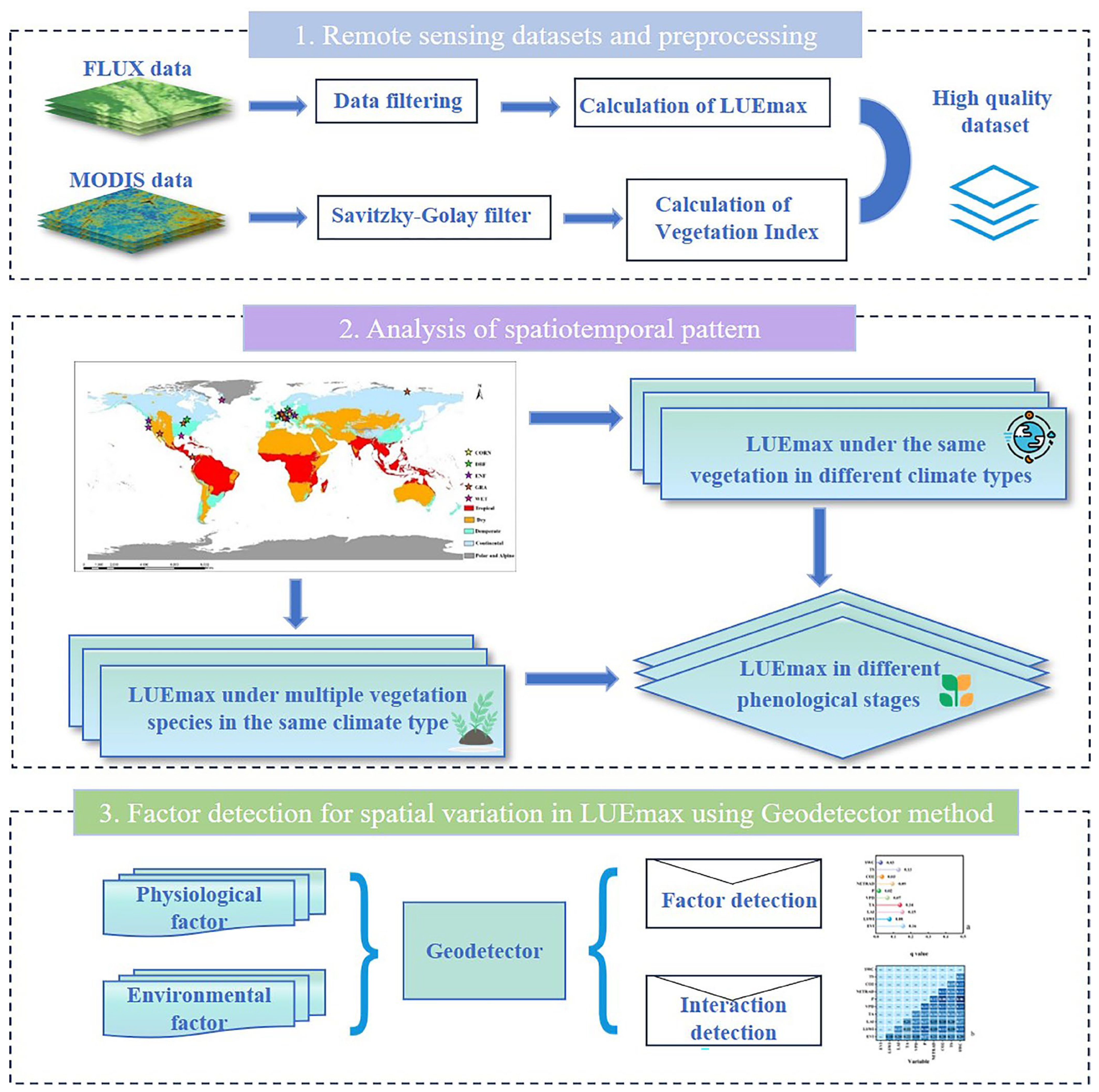
2. Materials and Methods

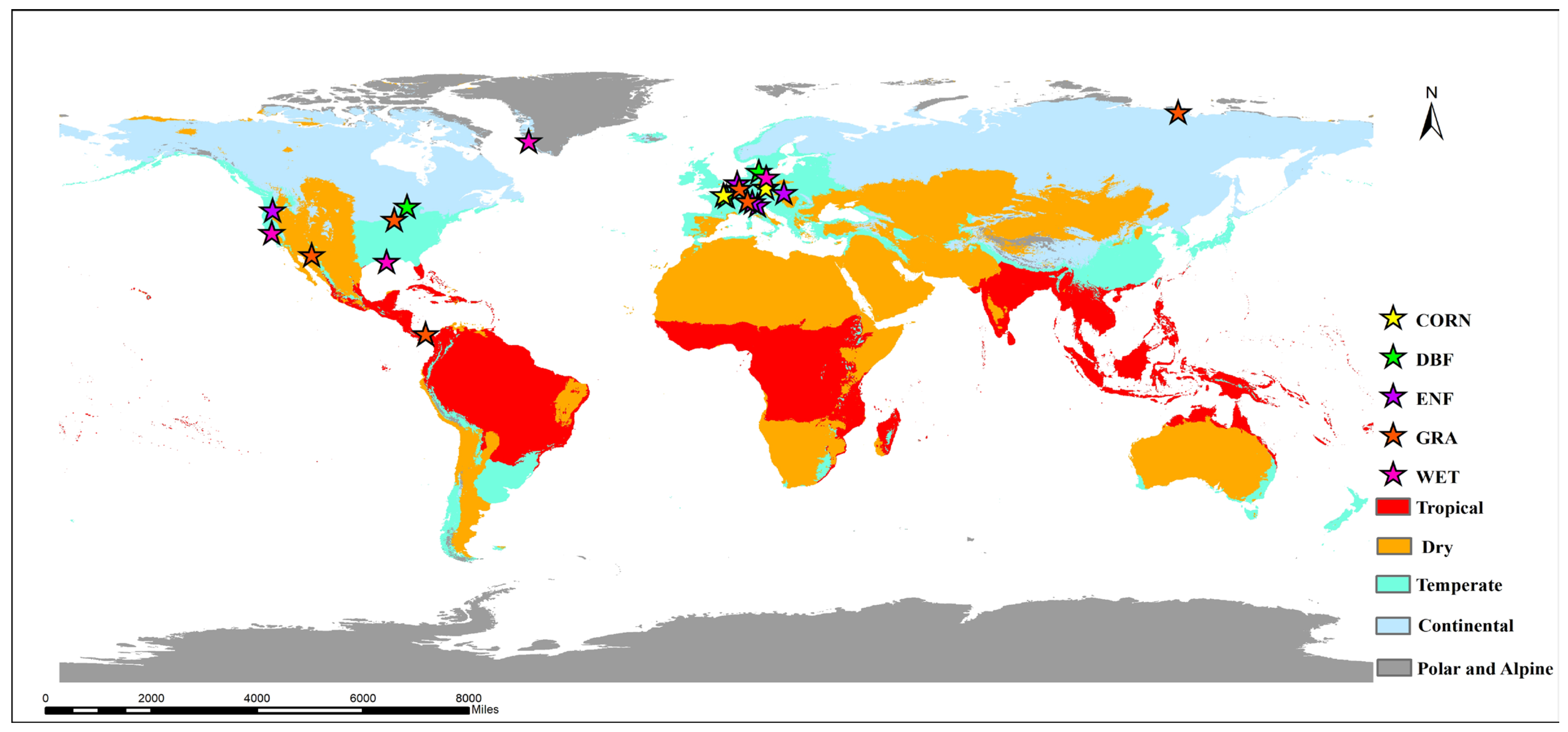
2.1. Study Sites

Flux sites, also known as eddy covariance stations, are research facilities that measure the exchange of energy, carbon, water vapor, and other gases between terrestrial ecosystems and the atmosphere. Considering the availability of data and the observation duration, 23 flux observation sites with high-quality data (Table 1) were selected. The study sites include evergreen needleleaf forests (ENF), deciduous broadleaf forests (DBF), grasslands (GRA), croplands (CORN), and wetlands (WET) spanning multiple Köppen–Geiger climate classifications [39,40,41]. Climate zones were stratified into the following five major classes: tropical, dry (including arid and semi-arid), temperate, continental, and polar/alpine (Figure 1). Tropical climates are characterized by consistently high temperatures and abundant rainfall, typically supporting lush vegetation. Dry climates experience low precipitation, with the conditions ranging from arid deserts to semi-arid steppes. Temperate climates feature moderate temperatures and distinct seasons, with sufficient rainfall to sustain diverse vegetation. Continental climates exhibit significant seasonal temperature variation, with cold winters and warm summers often found in inland regions. Polar and alpine climates are defined by persistently cold temperatures and limited precipitation, primarily occurring in high-latitude or high-altitude regions.

2.2. Data

2.2.1. Flux Data

FLUXNET 2015 synthesizes eddy covariance measurements from globally distributed regional networks [42,43]. This open-access dataset (https://fluxnet.org/data/fluxnet2015-dataset/, accessed on 16 December 2024) provides multi-temporal observations (half-hourly to yearly) of carbon, water, and energy fluxes from 212 globally distributed sites [43]. All records have undergone rigorous quality assurance procedures with standardized processing protocols to ensure cross-site consistency [43]. Sites with observations representing different vegetation types were used to directly compare the LUEmax’s patterns of change. Moreover, sites are strategically distributed across different climate zones, thereby facilitating the study of variations in LUEmax values under diverse environmental conditions during the same period. The variables used in this study include net ecosystem exchange (‘NEE_VUT_REF’), photosynthetic photon flux density incident (‘PPFD_IN’), vapor pressure saturation deficit (‘VPD_F’), air temperature (‘TA_F’), soil temperature (‘TS_F_MDS’), precipitation (‘P_F’), CO₂ mole fraction (‘CO_{2_}F_MDS’), and net radiation (‘NETRAD’). We refined high-quality data to eliminate abnormal data exhibiting PPFD_IN_QC values of −9999 or 0.

Table 1. Distribution of flux sites.

Site_ID	Latitude	Longitude	Köppen–Geiger Classification	Biome Type	Data Period	Reference
NL-Loo	52.1666	5.7436	temperate	ENF	2007–2009	[44]
US-Me2	44.4526	−121.5589	temperate	ENF	2013–2014	[45]
IT-Lav	45.9562	11.2813	continental	ENF	2007–2009	[46]
CZ-BK1	49.5021	18.5369	continental	ENF	2012–2014	[47]
CH-Dav	46.8153	9.8559	polar and alpine	ENF	2007–2009 2012–2014	[48]
PA-SPn	9.3181	−79.6346	tropical	DBF	2007–2008	[49]
FR-Fon	48.4764	2.7801	temperate	DBF	2007–2009	[50]
DK-Sor	55.4859	11.6446	temperate	DBF	2012–2014	[51]
US-UMd	45.5625	−84.6975	continental	DBF	2007–2009	[52]
US-UMB	45.5598	−84.7138	continental	DBF	2012–2014	[53]
PA-SPs	9.3138	−79.6314	tropical	GRA	2007–2009	[49]
US-SRG	31.7894	−110.8277	dry	GRA	2012–2014	[54]
DE-RuR	50.6219	6.3041	temperate	GRA	2012–2014	[55]
US-IB2	41.8406	−88.241	continental	GRA	2007–2009	[56]
DE-Gri	50.95	13.5126	continental	GRA	2012–2014	[57]
CH-Fru	47.1158	8.5378	polar and alpine	GRA	2007–2009	[58]
RU-Sam	72.3738	126.4958	polar and alpine	GRA	2012–2014	[59]
FR-Gri	48.8442	1.9519	temperate	CORN	2012–2014	[60]
DE-Kli	50.8931	13.5224	continental	CORN	2012–2014	[57]
US-Myb	38.0499	−121.765	temperate	WET	2012–2014	[61]
US-LA2	29.8587	−90.2869	temperate	WET	2012–2013	[62]
DE-Akm	53.8662	13.6834	continental	WET	2012–2014	[63]
GL-NuF	64.1308	−51.3861	polar and alpine	WET	2012–2014	[64]

Table 1. Distribution of flux sites.

Site_ID	Latitude	Longitude	Köppen–Geiger Classification	Biome Type	Data Period	Reference
NL-Loo	52.1666	5.7436	temperate	ENF	2007–2009	[44]
US-Me2	44.4526	−121.5589	temperate	ENF	2013–2014	[45]
IT-Lav	45.9562	11.2813	continental	ENF	2007–2009	[46]
CZ-BK1	49.5021	18.5369	continental	ENF	2012–2014	[47]
CH-Dav	46.8153	9.8559	polar and alpine	ENF	2007–2009 2012–2014	[48]
PA-SPn	9.3181	−79.6346	tropical	DBF	2007–2008	[49]
FR-Fon	48.4764	2.7801	temperate	DBF	2007–2009	[50]
DK-Sor	55.4859	11.6446	temperate	DBF	2012–2014	[51]
US-UMd	45.5625	−84.6975	continental	DBF	2007–2009	[52]
US-UMB	45.5598	−84.7138	continental	DBF	2012–2014	[53]
PA-SPs	9.3138	−79.6314	tropical	GRA	2007–2009	[49]
US-SRG	31.7894	−110.8277	dry	GRA	2012–2014	[54]
DE-RuR	50.6219	6.3041	temperate	GRA	2012–2014	[55]
US-IB2	41.8406	−88.241	continental	GRA	2007–2009	[56]
DE-Gri	50.95	13.5126	continental	GRA	2012–2014	[57]
CH-Fru	47.1158	8.5378	polar and alpine	GRA	2007–2009	[58]
RU-Sam	72.3738	126.4958	polar and alpine	GRA	2012–2014	[59]
FR-Gri	48.8442	1.9519	temperate	CORN	2012–2014	[60]
DE-Kli	50.8931	13.5224	continental	CORN	2012–2014	[57]
US-Myb	38.0499	−121.765	temperate	WET	2012–2014	[61]
US-LA2	29.8587	−90.2869	temperate	WET	2012–2013	[62]
DE-Akm	53.8662	13.6834	continental	WET	2012–2014	[63]
GL-NuF	64.1308	−51.3861	polar and alpine	WET	2012–2014	[64]

2.2.2. MODIS Data

MODIS products (MOD09A1, MOD15A2H) with 8-day composites and a 500 m resolution were used in this study (https://lpdaac.usgs.gov/products/mod09a1v061/ (accessed on 22 February 2024) [30]. MOD15A2H provides Leaf Area Index (LAI) data. MOD09A1 surface reflectance data, processed from MODIS Level 1B radiance measurements, contain the following seven spectral bands: red (620–670 nm), near-infrared (NIR1: 841–876 nm; NIR2: 1230–1250 nm), shortwave infrared (SWIR1: 1628–1652 nm; SWIR2: 2105–2155 nm), blue (459–479 nm), and green (545–565 nm) [65]. The Land Surface Water Index (LSWI) [66] and Enhanced Vegetation Index (EVI) [67] were derived from MOD09A1. A Savitzky–Golay filtering algorithm was applied to mitigate cloud-induced atmospheric noise in the time-series remote sensing data [68]. EVI and LSWI were calculated as follows:

$$EVI=G\times {\displaystyle \frac{{\rho }_{NIR}-{\rho }_{Red}}{{\rho }_{NIR}+\left(C_1\times {\rho }_{Red}-C_2\times {\rho }_{Blue}\right)+L}}$$

(1)

$$LSWI={\displaystyle \frac{{\rho }_{NIR}-{\rho }_{SWIR}}{{\rho }_{NIR}+{\rho }_{SWIR}}}$$

(2)

where ${\rho }_{NIR}$, ${\rho }_{Red}$, ${\rho }_{Blue}$, and ${\rho }_{SWIR}$ are the reflectances of the blue, red, near-infrared (NIR), and shortwave infrared (SWIR) bands, respectively, in Equation (1); G is set to 2.5, C₁ is set to 6, C₂ is set to 7.5, and L is set to 1.

2.2.3. Environmental Factors Data

Physiological mechanism factors (

Table 2. Influencing factors data.

Variable Type	Influencing Factor Variable
Physiological mechanism factor	Vegetation type
	Enhanced Vegetation Index (EVI)
	Leaf Area Index (LAI)
	Land Surface Water Index (LSWI)
Environmental mechanisms factor	Temperature of the Air (TA)
	Temperature of the Soil (TS)
	Vapor Pressure Deficit (VPD)
	Soil Water Content (SWC)
	Net Radiation (NETRAD)
	Carbon Dioxide Molar Fraction (CO2_F)
	Precipitation (P)

) were derived from the aforementioned MODIS products. Environmental mechanisms factor (Table 2) data were analyzed using the Fluxnet 2015 datasets. These datasets were standardized following the methods established by Fluxnet. The half-hourly data within the Fluxnet 2015 dataset were gap-filled using the MDS (marginal distribution sampling) method [69]. The 8-day vapor pressure saturation deficit (‘VPD_F’), air temperature (‘TA_F’), soil temperature (‘TS_F_MDS’), precipitation (‘P_F’), CO₂ mole fraction (‘CO₂_F_MDS’), net radiation (‘NETRAD’), and remote sensing data were utilized for studying the extent of the impact on the LUEmax.

2.3. Methods

The methodological framework of this study is systematically illustrated in Figure 2. This section elaborates on key data processing methods and LUEmax estimation.

2.3.1. Calculation of Maximum Light Use Efficiency

LUEmax, an inherent characteristic of vegetation, can be derived by fitting time-series data on net ecosystem exchange (NEE), ecosystem respiration (Re), and photosynthetically active radiation (PAR) using light response curves. This study utilized a rectangular hyperbolic function (Michaelis–Menten light-response equation) to fit the three parameters obtained from eddy covariance measurements.

$$NEE={\displaystyle \frac{LU{E}_{max}\times PAR\times GE{E}_{max}}{LU{E}_{max}\times PAR+GE{E}_{max}}}-Re$$

(3)

where Re is the daytime ecosystem respiration, and GEEmax represents the maximum rate of gross ecosystem photosynthesis (µmol CO₂·m⁻²·s⁻¹). In this study, daily and 8-day data on the LUEmax were calculated for studying the changes in regularity.

2.3.2. Physical Extraction Methods

There has been rapid development and wide utilization of the double logistic function (DLF) method for extracting phenological indices on a site or regional scale [30,70]. It is a common nonlinear function consisting of two logistic functions, with each function having an inflection point and a curvature parameter. The following logistic function was used to extract values for the start of the growing season (SOS) and the end of the growing season (EOS). The parameters for the DLF are adjustable to fit diverse ecosystem responses, making it highly adaptable to different ecosystem types and environmental conditions.

$$Y\left(t\right)={\alpha }_1+{\displaystyle \frac{{\alpha }_2}{1+e^{-{\partial }_1\left(t-{\beta }_1\right)}}}-{\displaystyle \frac{{\alpha }_3}{1+e^{-{\partial }_2\left(t-{\beta }_2\right)}}}$$

(4)

$$SOS={\beta }_1$$

(5)

$$EOS={\beta }_2$$

(6)

where Y(t) is the observed data value at time t for DOY (day of year). The value during the dormant winter period is represented by ${\alpha }_1$. The amplitude between the winter dormant period and the spring and early summer peak is given by ${\alpha }_2$–${\alpha }_1$, while the amplitude between the winter dormant period and the late summer and autumn peak is ${\alpha }_3$–${\alpha }_1.$ Curvature metrics ${\partial }_1$ and ${\partial }_2$ are utilized to adjust the slope of the logistic function. ${\beta }_1$ and ${\beta }_2$ are the inflection points of the DOY corresponding to the transitions of the vegetation green-up and senescence stages. The fitted parameters of ${\beta }_1$ and ${\beta }_2$ signify SOS and EOS, respectively. The length of the growing season is calculated as the difference between ${\beta }_1$ and ${\beta }_2$.

2.3.3. Trend Analysis

The LUEmax time-series data trend was analyzed using the Theil–Sen trend, with significance tested via the Mann–Kendall test [71]. The Sen’s slope ($\beta$) was calculated as follows:

$$\beta =Median\left({\displaystyle \frac{x_j-x_i}{j-i}}\right),\forall j>i$$

(7)

Here, $x_i$ and $x_j$ are the data values at time points $i$ and $j$ ($j>i$), respectively. The resulting slope ($\beta$) represents the rate of change, where a positive value indicates an increasing trend and a negative value suggests a decreasing trend.

The Mann–Kendall test, a non-parametric statistical approach, which has no requirement for compliance with a particular distribution and remains undisturbed by other abnormal values, was utilized to quantify the significance of the trend [72]. The significance of the trend is assessed based on the absolute value of Z. Confidence levels of 90%, 95%, and 99% correspond to thresholds of ∣Z∣ > 1.65, ∣Z∣ > 1.96, and ∣Z∣ > 2.58, respectively.

2.3.4. Geodetector

Spatial heterogeneity is one of the fundamental characteristics of geographical phenomena. Geodetector refers to statistical techniques employed to detect spatial variability and disclose the driving factors [73]. Geodetector comprises the following four components: risk, factor, ecological, and interaction detectors. The factor detector detects the spatially stratified heterogeneity (SSH) of dependent variable y (i.e., LUEmax value). It also measures the degree to which the independent variable x (which includes physiological and environmental mechanism factors) can explain the SSH of the y value. It is expressed as follows:

$$q=1-{\displaystyle \frac{{{\displaystyle \sum }}_{h=1}^L{N}_h{\sigma }_h^2}{N{\sigma }^2}}$$

(8)

where L represents the stratification of the dependent variable, LUEmax, or the influence factor X; N and N_h are the number of sample units in strata h and the total region, respectively; and ${\sigma }_h^2$ and ${\sigma }^2$ are the variance in the h strata and the variance in the region. Generally, a larger value implies a stronger explanatory power of each factor. This study used the q value to quantify the explanatory degree of different drivers.

Climatic and ecological factors closely associated with variations in the LUEmax were chosen as the factors influencing LUEmax. Ten environmental factors, namely, remote sensing indices (EVI, LSWI, and LAI), air temperature, soil temperature, VPD, precipitation, CO₂ molar fraction, and net radiation, were selected to analyze their relationship with LUEmax’s change rate. Several discretization methods are available in the R language, including natural discontinuity and equal-interval discretization [74]. The parameter values for discretization grouping were set accordingly. The optimal combination of discretization methods and parameter values was determined through comparative analysis. Because the Geodetector algorithm works on discrete data, the ten continuous independent variables were transformed into discrete categories using an optimal method. Finally, the discretized data were used to perform calculations in Geodetector for factor and interaction detection.

3. Results

3.1. Spatiotemporal Dynamic Variation Pattern in LUEmax

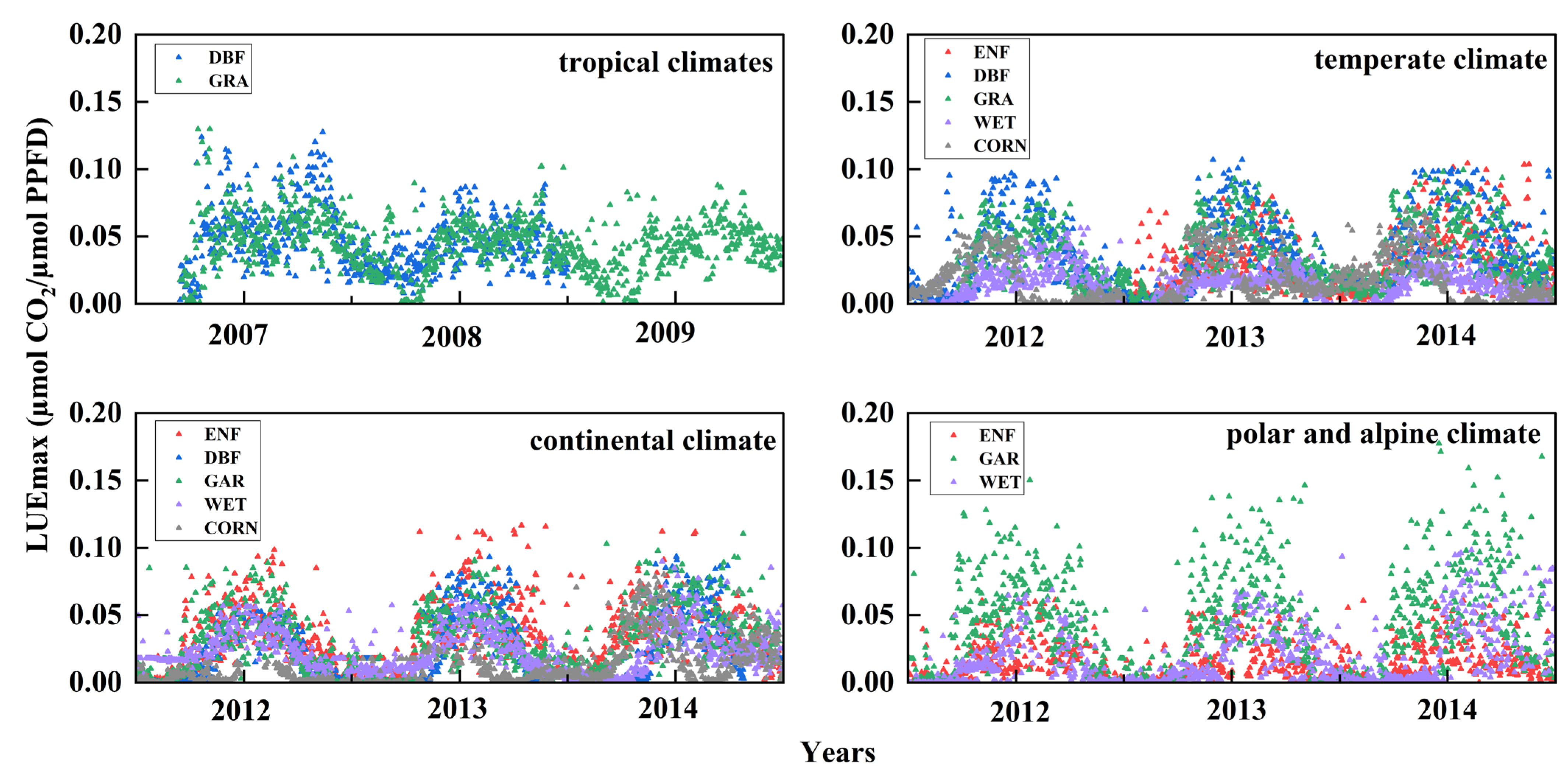
3.1.1. Temporal Dynamics of LUEmax for the Same Vegetation in Different Climate Types

The LUEmax values for the same vegetation type exhibited significant spatiotemporal heterogeneity in different climate zones (Figure 3). Over the study period, the annual average LUEmax values were 0.084 ± 0.025 µmol CO₂/µmol PPFD for ENF, 0.078 ± 0.05 µmol CO₂/µmol PPFD for DBF, 0.08 ± 0.05 µmol CO₂/µmol PPFD for GRA, 0.06 ± 0.04 µmol CO₂/µmol PPFD for WET, and 0.05 ± 0.03 µmol CO₂/µmol PPFD for CORN. The LUEmax values of ENF showed notable variations across temperate, continental, and polar and alpine climate types, with lower average values for polar and alpine types but higher fluctuations and peaks. DBF displayed higher LUEmax values with pronounced peaks in tropical areas, while temperate and continental aeras exhibited more stable, moderate values. Significant interannual variability was observed for GRA, with polar and alpine climates exhibiting the highest peaks and greatest variability. CORN showed consistently lower LUEmax values, with slightly higher peaks in continental compared to temperate climate types. WET exhibited relatively stable and low LUEmax values across temperate, continental, and polar and alpine climates, with polar and alpine zones showing slightly more significant variability and peaks.

This may be due to photosynthesis in ENF being limited by low temperatures and short growing seasons in polar and alpine regions, resulting in a low average LUEmax. DBF undergo intense photosynthesis in tropical areas due to the abundant light and heat, leading to high LUEmax values with peaks. The stable climate conditions in temperate and continental regions result in moderate LUEmax values. GRA are sensitive to the environment and show significant peaks and inter-annual variations in polar and alpine climates. CORN have little photosynthetic potential and poor adaptability, leading to a low overall LUEmax value. WET prefer a mild and stable environment, and their LUEmax values were low and stable across various climates, with slightly greater variability and peaks in polar and alpine regions.

These results highlight that the LUEmax values for the same vegetation type vary for different climate types, reflecting the influence of climatic conditions on photosynthetic efficiency. Generally, wetter or more variable climates (e.g., polar and alpine climates) are associated with greater fluctuations and peaks in the LUEmax. Conversely, more stable climates (e.g., temperate climates) tend to show lower and more consistent LUEmax values. These patterns underscore the importance of considering climatic variability when understanding ecosystem productivity and carbon cycling.

3.1.2. Temporal Dynamics of LUEmax Across Multiple Vegetation Species in the Same Climate Type

The LUEmax values across different vegetation types exhibited significant spatiotemporal heterogeneity within the same climate zones (Figure 4). In tropical climates, the LUEmax values for DBF and GRA showed noticeable fluctuations. GRA generally exhibited higher LUEmax values than DBF, with significant interannual variability and distinct peaks. DBF maintained relative stability and small peaks. All vegetation types (ENF, DBF, GRA, WET, and CORN) demonstrated notable variability in their LUEmax values in temperate climates. ENF and DBF exhibited higher LUEmax values and more pronounced peaks than other vegetation types. GRA and WET maintained moderate levels of LUEmax, while CORN consistently showed lower values. ENF showed the highest LUEmax values in continental climates, with frequent and sharp peaks over time. DBF and GRA also demonstrated relatively high LUEmax values but with more minor fluctuations. WET and CORN displayed the lowest LUEmax values, with WET showing slightly more variability than CORN. WET consistently exhibited the highest LUEmax values in polar and alpine climates, characterized by substantial fluctuations and peaks. ENF and DBF showed moderate LUEmax values, while GRA and WET had lower levels, with less variability and fewer pronounced peaks.

The results reveal that LUEmax values vary significantly across vegetation types within the same climate type, reflecting differences in vegetation’s physiological and ecological responses to climatic conditions. ENF and DBF generally exhibited higher LUEmax in temperate and continental climates, while WET dominated in polar and alpine climates. GRA maintained moderate values across most climates, whereas CORN showed consistently lower LUEmax across climate zones.

3.1.3. Spatial Dynamics of the LUEmax

The experimental results show the variations in LUEmax during different growth periods (

Table 3. Statistical results of the Sen trend analysis and M-K test. The results were classified into the following: very significant increase (VSI); significant increase (SI); slightly significant increase (SSI); no significant increase (NSI); invariant (I); no significant decrease (NSD); slightly significant decrease (SSD); significant decrease (SD); very significant decrease (VSD).

Site_ID	Climate Type	Vegetation Type	Before SOS	SOS-Peak	Peak-EOS	After EOS
NL-Loo	temperate	ENF	NSI	VSI	VSD	SSD
US-Me2	temperate	ENF	VSI	VSI	NSD	VSD
IT-Lav	continental	ENF	VSI	VSD	SD	VSD
CZ-BK1	continental	ENF	VSI	SSI	SD	VSD
CH-Dav	polar and alpine	ENF	NSI	VSI	NSD	NSD
PA-SPn	tropical	DBF	NSI	NSI	NSD	SSD
FR-Fon	temperate	DBF	VSI	SI	SSD	VSD
DK-Sor	temperate	DBF	SI	VSI	VSD	VSD
US-UMd	continental	DBF	NSI	VSI	VSD	VSD
US-UMB	continental	DBF	VSI	NSI	NSD	NSD
PA-SPs	tropical	GRA	NSI	VSI	VSI	SSD
US-SRG	dry	GRA	VSI	SSI	SD	VSD
DE-RuR	temperate	GRA	SD	VSI	VSD	VSI
US-IB2	continental	GRA	VSI	NSI	SI	NSD
DE-Gri	continental	GRA	SSI	NSI	NSI	NSD
CH-Fru	polar and alpine	GRA	NSI	VSI	NSD	VSD
RU-Sam	polar and alpine	GRA	SSI	VSI	VSD	NSD
FR-Gri	temperate	CORN	VSI	SSI	SD	VSI
DE-Kli	continental	CORN	SI	NSI	VSD	SSI
US-Myb	temperate	WET	NSD	NSI	NSI	VSD
US-LA2	temperate	WET	NSI	NSI	NSD	VSD
DE-Akm	continental	WET	VSI	NSI	VSD	SSI
GL-NuF	polar and alpine	WET	NSI	VSI	NSD	SSI

). In tropical climates, the LUEmax of GRA increased significantly during the SOS-Peak period, while the change in DBF was relatively small. Both showed a slight increase in the later stage of the growing season. In dry climates, the LUEmax of GRA rose rapidly during the early stage of the growing season but declined substantially in the later stage. In temperate climate types, the LUEmax of ENF and GRA increased significantly during the SOS-Peak stage of the growing season but dropped sharply after the growing season ended. The trend for DBF was similar, while WET had relatively small changes across all stages and mainly decreased in the late growing season. For the continental climate type, the LUEmax of ENF increased significantly during the Before SOS period but declined rapidly during the middle and late stages of the growing season. For DBF, they showed a significant increase from the SOS-Peak stage and then dropped quickly. In contrast, the LUEmax values for GRA and CORN changed relatively smoothly throughout the growing season, with only minor fluctuations in the middle and later periods. For the polar and alpine climate types, the LUEmax of ENF increased significantly during the SOS-Peak period, with little change in other periods. For GRA and WET, LUEmax decreased during the Peak-EOS stage but slightly recovered after the end of the growing season.

These results emphasize that climatic conditions significantly influence the variation patterns in LUEmax during the different vegetation growth periods. These variation characteristics of LUEmax across different vegetation types reflect their adaptability to the respective growing environments. In temperate and continental climates, the LUEmax showed a large-scale increase and decrease in the middle of the growing season and mainly presented a declining trend after the end of the growing season. In polar and alpine climates, the LUEmax changed relatively smoothly. In tropical and arid climates, the LUEmax changed steadily.

3.2. Impact of Factors on the LUEmax

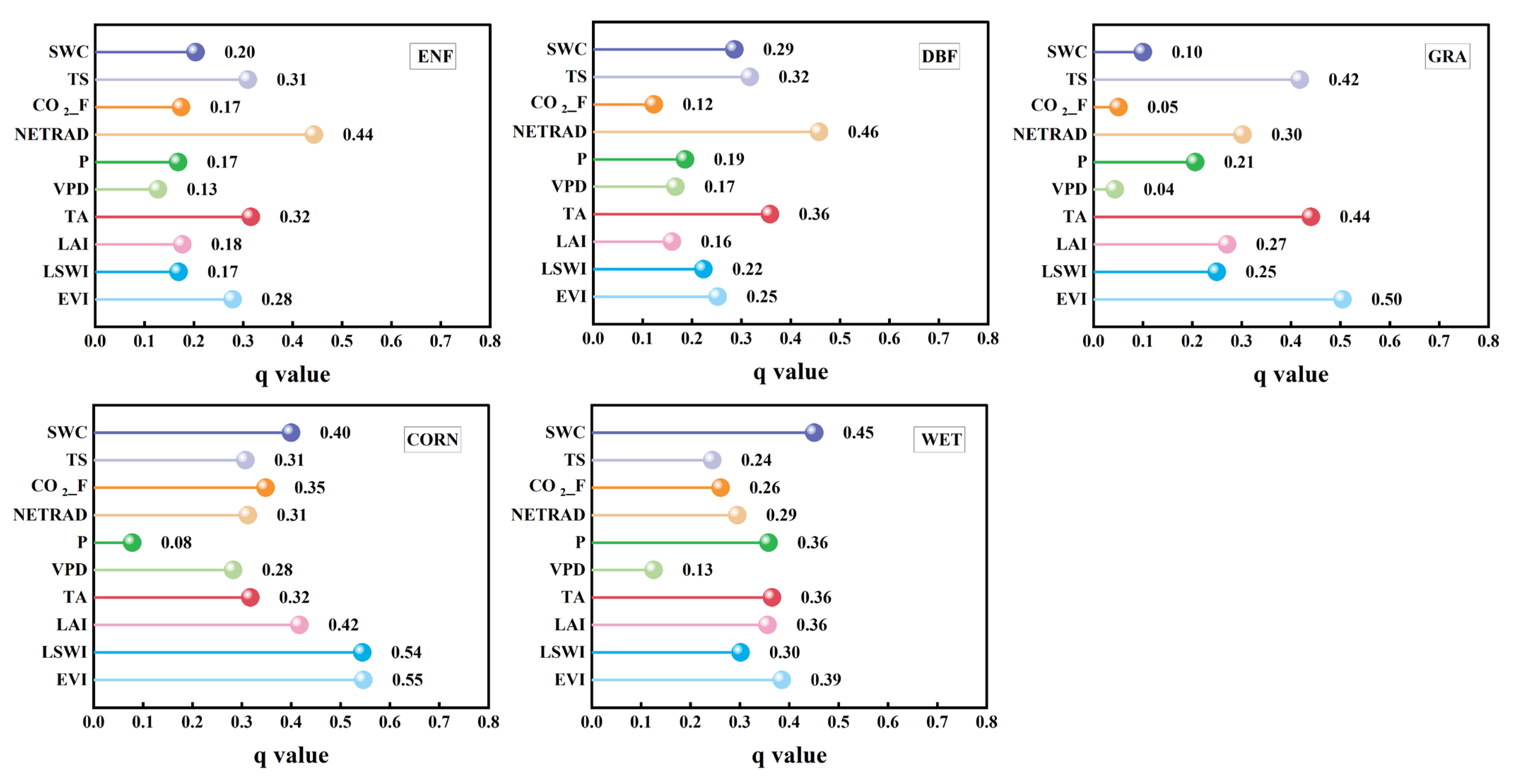
3.2.1. Impact of Factors on the LUEmax Across Different Vegetation Types

The factor detector in the Geodetector model was used to analyze the extents of the impacts of ten factors (EVI, LSWI, LAI, TA, TS, VPD, P, SWC, CO₂_F, and NETRAD) on the LUEmax. The results show the explanatory power of each factor for the spatial differentiation of the LUEmax (Figure 5). All environmental factors influenced the spatial variability of the LUEmax at a statistically significant level (p < 0.05). The variability in the LUEmax impact factors was significant across different vegetation types.

For ENF, the most significant factor for LUEmax was the NETRAD, followed by TA and TS, indicating their sensitivity to atmospheric and climatic conditions. The LUEmax of DBF is mainly affected by the NETRAD and TA, reflecting their temperature dependence. EVI is the key driving factor of the LUEmax of GRA, while TS and TA also play important roles. For WET, the LUEmax is mainly influenced by the SWC, EVI, and TA, emphasizing its dual dependence on vegetation cover density and temperature conditions. For CORN, EVI is the primary factor. Meanwhile, the LSWI and LAI are also important influence factors.

These findings underscore that significant differences exist in the influence of various factors on the LUEmax among different vegetation types. The impact of the NETRAD is more prominent for ENF and DBF, while it is relatively small in other vegetation types. TS has a more significant influence in ENF, DBF, and CORN. The influence of CO₂_F is relatively small among all vegetation types. Other factors, such as SWC, P, VPD, TA, LAI, LSWI, and EVI, have effects of varying extents on the LUEmax among different vegetation types.

The interaction detector was utilized to gauge the extent to which factor interactions can explain the spatial variation in LUEmax across various vegetation types, as illustrated in Figure 6. When the q value of the interaction between two factors exceeds the higher q value of either factor (X1 or X2) but remains lower than their sum, this indicates a mutual enhancement effect. If the q value of their interaction surpasses the sum of both individual q values, this suggests a nonlinear enhancement between the two factors. The results of this study indicate that the q value for any two-factor interaction in the spatial variation in LUEmax exceeded that of a single factor, suggesting that the explanatory power of individual factors increases when they interact. Moreover, the combined effect of two factors on the LUEmax’s spatial variation was stronger than that of either factor alone.

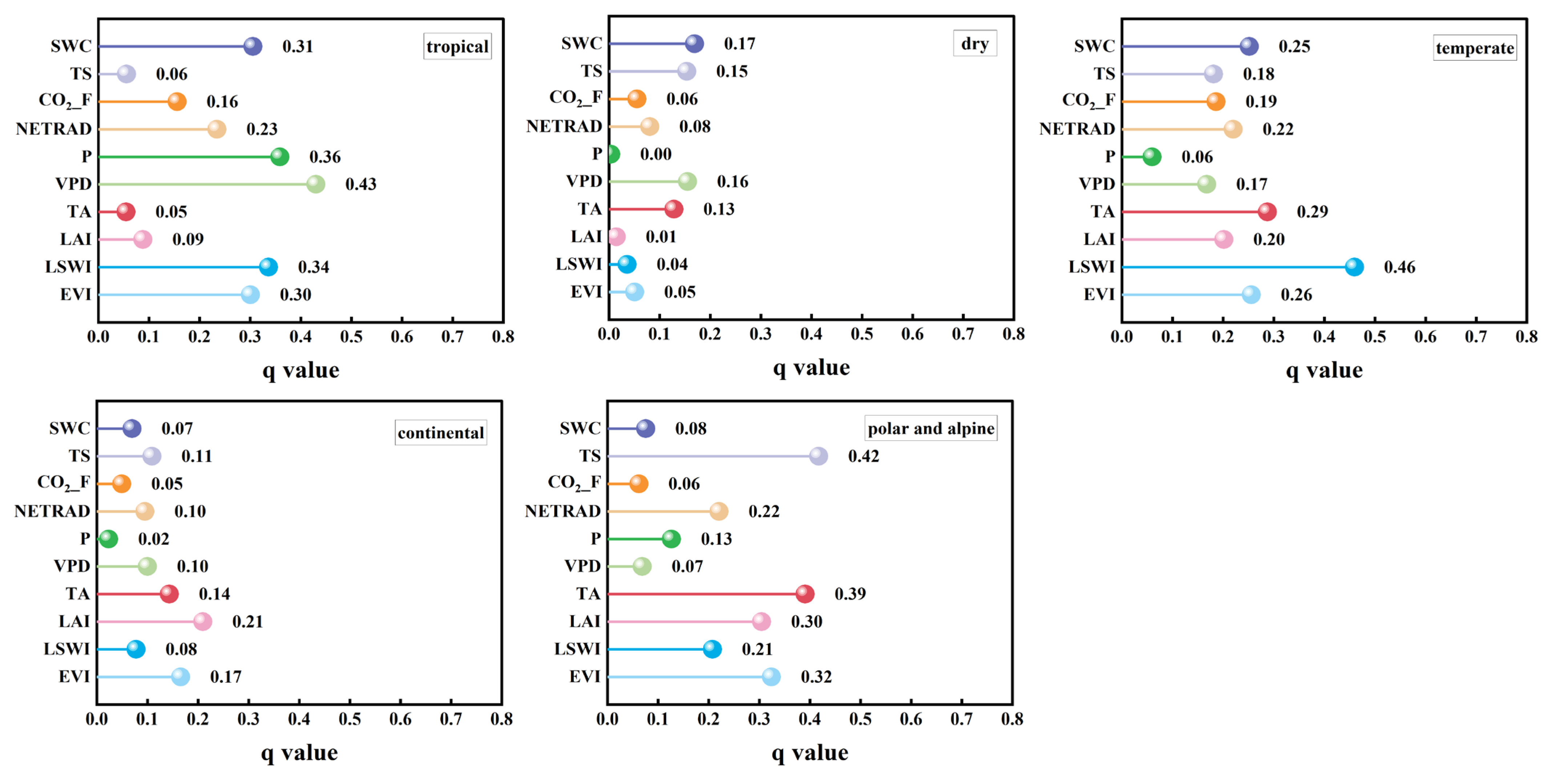
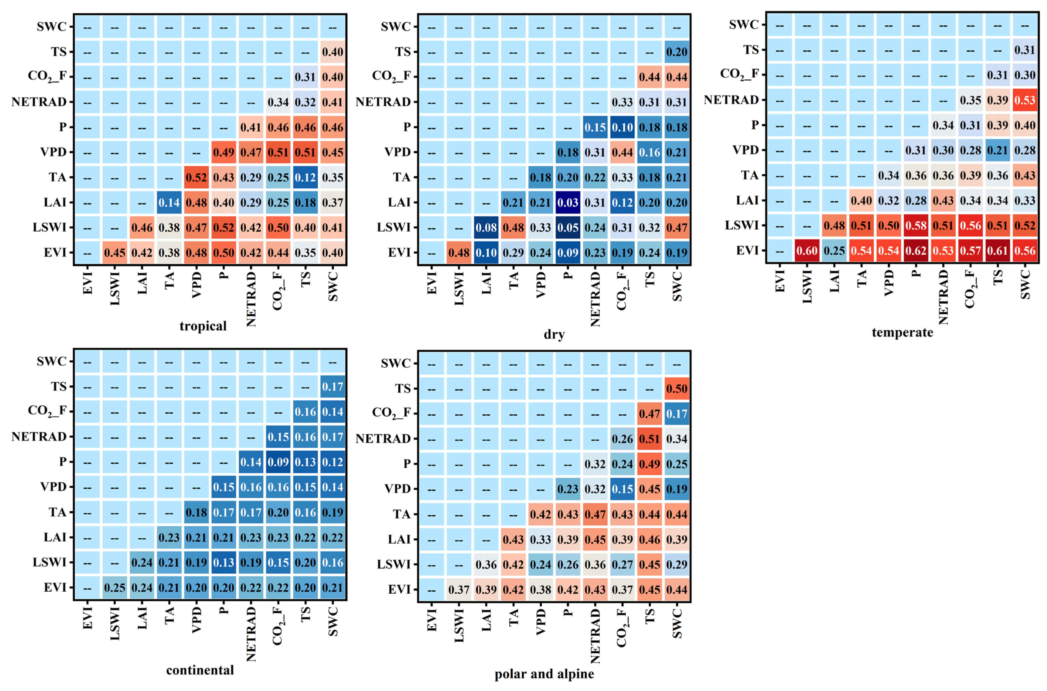
3.2.2. Impact of Factors on the LUEmax Across Different Climate Types

Geodetector’s factor detector was employed to assess the influence of ten factors on the LUEmax in different climates. The results show the explanatory power of each factor on the spatial differentiation of LUEmax (Figure 7). The variability of the LUEmax image factors was significant for different climates.

In tropical climates, both P and VPD strongly influence LUEmax, suggesting that these two factors are the primary controllers of LUEmax in tropical regions. In dry climates, the degrees of influence of all factors are relatively low. This may be due to the limited water in arid areas, which leads to minor impacts of other factors. In temperate climates, the main influencing factor of LUEmax is LSWI, followed by TA. This is related to this region’s relative water demand and climate change characteristics. In continental climates, LUEmax is mainly affected by the LAI, while the influences of other factors are rather limited. In polar and alpine climates, the TS and TA responses are significant, and the influence of EVI cannot be ignored either, although the overall impact is relatively small.

The interaction detector assessed the explanatory power of factor interactions in LUEmax spatial variation across different climate types (Figure 8). Within different climate types, the interaction of two factors had a greater influence on LUEmax’s spatial variation than either factor alone.

These results demonstrate the substantial differences in the interaction relationships and influence degrees among environmental factors across different climate types. These differences reflect the impacts of the specific environmental conditions in each climate zone on the LUEmax.

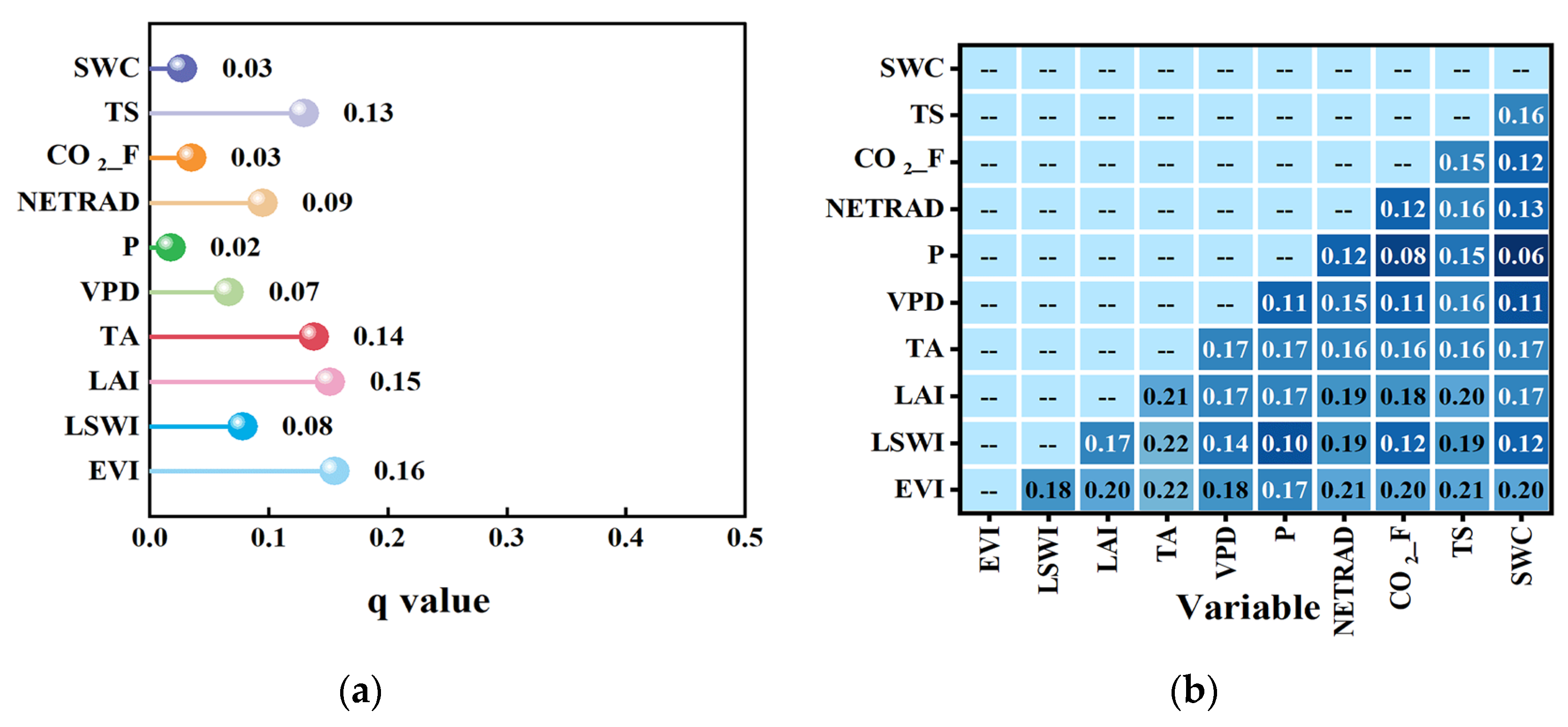
3.2.3. Impact of Factors on the LUEmax

The results show the explanatory power of each factor on the spatial differentiation of the LUEmax and assess the explanatory power of factor interactions on the LUEmax (Figure 9). The geographical detector’s factor detection and interaction detection results show that the impacts of the different factors on the LUEmax vary significantly. Regarding the influence of single factors, LAI and VPD were the main driving factors affecting the LUEmax, indicating that vegetation conditions and atmospheric humidity greatly impact the LUEmax. Variables such as SWC, CO₂_F, and TA have moderate influences, reflecting that soil moisture, carbon dioxide concentration, and air temperature also affect the LUEmax. The influences of P and NETRAD were relatively low, indicating that these factors have a weak direct effect on the LUEmax.

Further analysis of the interaction among factors reveals that the combined effect of two factors is significantly greater than that of a single factor effect, suggesting that LUEmax is jointly driven by multiple environmental factors. In particular, the interaction effects of combinations such as TA and EVI and TA and LSWI are the most significant, reflecting a strong correlation between vegetation indices and climate factors. These results indicate that, in addition to the direct influence of individual factors, the change in the LUEmax is also significantly affected by the interaction of multiple factors, especially the coupling effect between vegetation indices and climate factors.

4. Discussion

4.1. Dynamics of the LUEmax

The LUEmax is a fundamental characteristic of plants [75]. However, at different scales, the LUEmax of vegetation is mainly influenced by species, growth stage at the leaf level, and light intensity, which may cause it to show obvious spatial heterogeneity [76]. According to the findings of this paper, the LUEmax varies significantly across different growth stages and under various growth conditions. During the early growth stages of plants, the LUEmax tends to be relatively low, as young plants have not yet fully developed their photosynthetic systems. As plants grows, the LUEmax gradually increases, reaching its peak during the growth cycle. This change reflects plants’ ability to continually optimize its photosynthetic system throughout the growth process. Each biome possesses structural characteristics unique to its environment [77]. For example, shrublands typically feature sparse, open canopies with short plants, smaller leaves, and predominantly sunlit foliage. In contrast, evergreen broadleaf forests are dense, with minimal gaps, tall trees, and larger leaves, resulting in a high proportion of shaded leaves. The LUEmax of plants presents obvious spatial heterogeneity and varies for different vegetation cover types [2]. Research on cropland and mangrove forests has demonstrated that LUEmax differs among various vegetation types and exhibits dynamic changes across different seasons. Specifically, these results show that LUEmax varies among crop types and is dynamic within a crop season. LUEmax undergoes dynamic seasonal variations in different climatic environments even for the same vegetation type [78,79]. This finding is in agreement with the results obtained in this study. According to the findings of this paper, herbaceous plants generally show lower LUEmax values, while tree species tend to have higher LUEmax values. The variability in LUEmax across different vegetation types reflects the distinct physiological and ecological strategies adapted to their specific environmental conditions. Ecosystems with the same vegetation type exhibit similar LUEmax variations despite significant spatiotemporal differences [80], indicating the feasibility and reliability of upscaling site-based LUEmax for regional or global GPP prediction. These differences highlight the dynamics of LUEmax, enabling models to better capture the adaptive responses of leaves to short-term environmental fluctuations [81].

4.2. Factors Affecting the Dynamics of LUEmax

Previous studies have shown that dynamic LUEmax values allow the model to better fit the adaptive response of leaves to short-term environmental changes, thus facilitating a more accurate calculation of gross primary productivity [81]. However, the LUEmax parameter is closely related to the physiological state of vegetation. In addition to factors such as temperature, LAI, and moisture, the nutrient element limitation, tree age, and proportion of diffuse radiation also affect it. The difference in LUEmax values may be caused by the seasonal variation characteristics of the original study area being limited by its single local climate. On the other hand, it may also result from the differences in community species within the same vegetation type. Studies have pointed out that the seasonal variation in the LUEmax parameter is closely related to the LAI and canopy structure [82], and the change in its value can be explained by ambient temperature [83,84]. Many studies have examined the interannual variations and seasonal dynamics of LUEmax, revealing that its fluctuations are influenced by environmental factors, such as radiation variability, vapor pressure deficit (VPD), and temperature [34,85].

Consistent with the findings in this study, previous research has demonstrated that TA, TS, NETRAD, VPD, LSWI, and EVI are important drivers of LUEmax. At the same time, the extent of their relative importance differs depending on the specific vegetation type and environmental context. These studies also found that different plant species exhibit significant differences in LUEmax. Forest ecosystems, such as ENF and DBF, depend strongly on radiation and TS conditions, while GRA and croplands (CORN) are more sensitive to the EVI and TA. WET show a reliance on the EVI and LAI. The interplay between environmental (e.g., temperature, radiation, VPD, and CO₂_F) and biophysical factors (e.g., LAI and EVI) drives the dynamic variation in LUEmax across different vegetation types. These findings demonstrate that the drivers of LUEmax are highly vegetation-specific, shaped by the interactions between environmental conditions and ecosystem functional traits. Among these factors, except the CFlux light-use efficiency model [86], which considers the tree age factor, most single-leaf light-use efficiency models do not have corresponding model parameter designs for the remaining factors. Therefore, adding model parameters for factors affecting LUEmax in the existing model structure and simultaneously calibrating all model parameters uniformly will help improve the accuracy of GPP estimations by the light-use efficiency model.

4.3. Limitations and Perspectives of the Study

The dynamic nature of LUEmax is posited to enhance the model’s alignment with the adaptive responses of foliage to transient environmental conditions, thereby facilitating more precise estimations of GPP. However, the LUEmax parameter is intricately linked to the physiological conditions of vegetation, influenced not only by temperature, LAI, and water availability but also by factors such as nutrient constraints, forest maturity, and the ratio of diffuse radiation. Nonetheless, many single-leaf light energy utilization models lack the corresponding parameterization for these influential factors. Consequently, incorporating parameters that account for these determinants of LUEmax into the existing model’s framework could significantly enhance the accuracy of VPM model predictions.

Light-response parameters characterize the photosynthetic light-response curve (LRC), which is essential in terrestrial carbon models [87]. The continuous expansion of the network of flux observation towers has provided valuable opportunities for research on light-response parameters at the ecosystem scale [88]. However, flux data are frequently affected by measurement errors. These errors stem from multiple factors, including meteorological conditions during data collection, sensor accuracy, and environmental fluctuations [89]. The estimation of LUEmax typically depends on light-response curves (LRC). Errors in flux data can, thus, compromise the accuracy of the LRC [90]. Moreover, the estimation of LUEmax is based on certain assumptions regarding the photosynthetic mechanisms in plants. These assumptions may deviate from the actual situation under different ecosystems and climate conditions. Additionally, uncertainties can be introduced by various aspects, such as the method of fitting the LRC, the selection of light intensity, and the interaction of other environmental variables [91].

The study above illustrates the dynamic variations in LUEmax across diverse vegetation types within different climatic regimes. However, because of the inadequacy of flux data across all climate classifications, the behavioral patterns in LUEmax for certain vegetation types in data-sparse climatic areas remain to be elucidated, along with the influence of other geographical environmental variables on LUEmax. Additionally, the methodologies employed to compute LUEmax are heterogeneous, leading to disparate estimations from various approaches. Future investigations should consider the seasonal fluctuations of LUEmax and the constraints imposed by climatic and environmental factors when modeling GPP with the LUE framework. This study predominantly draws upon data from the FUENET 2015 flux sites; however, the distribution and quantity of these sites are not uniformly representative across vegetation types. Therefore, further research is warranted, emphasizing the expansion of flux observations and integrating novel methodologies or tools, such as unmanned aerial remote sensing, the Chlorophyll Fluorescence Index (SIF), and the Photochemical Reflectance Index (PRI).

5. Conclusions

The LUEmax values were quantified using data from 23 global flux stations, and the change patterns in LUEmax across various vegetation types and climate zones were analyzed. The extent of the significant increases or decreases in LUEmax during different phenological stages of vegetation growth was evaluated using trend analysis methods. The contribution rates of environmental factors were determined using the Geodetector method. The key findings and conclusions are as follows: (1) LUEmax of the same vegetation type varies across different climate types. The annual average LUEmax values were 0.084 ± 0.025 µmol CO₂/µmol PPFD for ENF, 0.078 ± 0.05 µmol CO₂/µmol PPFD for DBF, 0.08 ± 0.05 µmol CO₂/µmol PPFD for GRA, 0.06 ± 0.04 µmol CO₂/µmol PPFD for WET, and 0.05 ± 0.03 µmol CO_2/µmol PPFD for CORN. (2) The LUEmax varies significantly across different growth stages and under various growth conditions. During the early growth stages of plants, the LUEmax tends to be relatively low, as young plants have not yet fully developed their photosynthetic systems. As the plant grows, the LUEmax gradually increases, reaching its peak during the growth cycle. More variable climates (e.g., polar and alpine climates) are associated with greater fluctuations and peaks in LUEmax. Conversely, more stable climates (e.g., temperate climates) tend to show lower LUEmax values. (3) The mechanisms influencing the LUEmax of different vegetation types vary significantly across diverse environmental conditions. The LUEmax of forests (ENF and DBF) are largely influenced by temperature and radiation, while grasslands and wetlands are more responsive to vegetation indices and hydrological factors. CORN exhibits a unique sensitivity to EVI and temperature conditions. The results show that various influencing factors have different combined effects on the LUEmax of different vegetation types. Radiative and TA combinations predominantly influence ENF and DBF, while CORN and WET show a stronger dependency on SWC and EVI factors. GRA demonstrates a unique sensitivity to EVI and TA. The findings of this study play an important role in advancing the theoretical development of gross primary productivity (GPP) models and enhancing the accuracy of carbon sequestration simulations in terrestrial ecosystems.

References

1. As-syakur, A.R.; Osawa, T.; Adnyana, I.W.S. Medium Spatial Resolution Satellite Imagery to Estimate Gross Primary Production in an Urban Area. Remote Sens. 2010, 2, 1496–1507. [Google Scholar] [CrossRef]
2. Li, A.; Bian, J.; Lei, G.; Huang, C. Estimating the Maximal Light Use Efficiency for Different Vegetation through the CASA Model Combined with Time-Series Remote Sensing Data and Ground Measurements. Remote Sens. 2012, 4, 3857–3876. [Google Scholar] [CrossRef]
3. Hilker, T.; Coops, N.C.; Wulder, M.A.; Black, T.A.; Guy, R.D. The use of remote sensing in light use efficiency based models of gross primary production: A review of current status and future requirements. Sci. Total Environ. 2008, 404, 411–423. [Google Scholar] [CrossRef]
4. Monteith, J.L. Solar radiation and productivity in tropical ecosystems. J. Appl. Ecol. 1972, 9, 747–766. [Google Scholar] [CrossRef]
5. Madani, N.; Kimball, J.S.; Affleck, D.L.; Kattge, J.; Graham, J.; Van Bodegom, P.M.; Reich, P.B.; Running, S.W. Improving ecosystem productivity modeling through spatially explicit estimation of optimal light use efficiency. J. Geophys. Res. Biogeosciences 2014, 119, 1755–1769. [Google Scholar] [CrossRef]
6. Dong, T.; Liu, J.; Qian, B.; Jing, Q.; Croft, H.; Chen, J.; Wang, J.; Huffman, T.; Shang, J.; Chen, P. Deriving Maximum Light Use Efficiency From Crop Growth Model and Satellite Data to Improve Crop Biomass Estimation. IEEE J. Sel. Top. Appl. Earth Obs. Remote Sens. 2017, 10, 104–117. [Google Scholar] [CrossRef]
7. Bartlett, D.S.; Whiting, G.J.; Hartman, J.M. Use of vegetation indices to estimate indices to estimate intercepted solar radiation and net carbon dioxide exchange of a grass canopy. Remote Sens. Environ. 1989, 30, 115–128. [Google Scholar] [CrossRef]
8. Zhao, C.; Zhu, W.; Xie, Z. Comparative evaluation of simulation methods for the maximum light-use efficiency of vegetation. J. Remote Sens. 2024, 28, 649–660. [Google Scholar] [CrossRef]
9. Pei, Y.; Dong, J.; Zhang, Y.; Yuan, W.; Doughty, R.; Yang, J.; Zhou, D.; Zhang, L.; Xiao, X. Evolution of light use efficiency models: Improvement, uncertainties, and implications. Agric. For. Meteorol. 2022, 317, 108905. [Google Scholar] [CrossRef]
10. Gan, R.; Zhang, L.; Yang, Y.; Wang, E.; Woodgate, W.; Zhang, Y.; Haverd, V.; Kong, D.; Fischer, T.; Chiew, F.; et al. Estimating ecosystem maximum light use efficiency based on the water use efficiency principle. Environ. Res. Lett. 2021, 16, 104032. [Google Scholar] [CrossRef]
11. Yuan, W.; Cai, W.; Xia, J.; Chen, J.; Liu, S.; Dong, W.; Merbold, L.; Law, B.; Arain, A.; Beringer, J.; et al. Global comparison of light use efficiency models for simulating terrestrial vegetation gross primary production based on the LaThuile database. Agric. For. Meteorol. 2014, 192–193, 108–120. [Google Scholar] [CrossRef]
12. Potter, C.S.; Randerson, J.T.; Field, C.B.; Matson, P.A.; Vitousek, P.M.; Mooney, H.A.; Klooster, S.A. Terrestrial ecosystem production: A process model based on global satellite and surface data. Glob. Biogeochem. Cycles 1993, 7, 811–841. [Google Scholar] [CrossRef]
13. Myneni, R.B.; Los, S.O.; Asrar, G. Potential gross primary productivity of terrestrial vegetation from 1982–1990. Geophys. Res. Lett. 1995, 22, 2617–2620. [Google Scholar] [CrossRef]
14. Lobell, D.B.; Hicke, J.A.; Asner, G.P.; Field, C.B.; Tucker, C.J.; Los, S. Satellite estimates of productivity and light use efficiencyin United States agriculture. Glob. Change Biol. 2002, 8, 722–735. [Google Scholar] [CrossRef]
15. Wang, H.; Jia, G.; Fu, C.; Feng, J.; Zhao, T.; Ma, Z. Deriving maximal light use efficiency from coordinated flux measurements and satellite data for regional gross primary production modeling. Remote Sens. Environ. 2010, 114, 2248–2258. [Google Scholar] [CrossRef]
16. Wang, M.; Sun, R.; Zhu, A.; Xiao, Z. Evaluation and Comparison of Light Use Efficiency and Gross Primary Productivity Using Three Different Approaches. Remote Sens. 2020, 12, 1003. [Google Scholar] [CrossRef]
17. Zhao, M.; Heinsch, F.A.; Nemani, R.R.; Running, S.W. Improvements of the MODIS terrestrial gross and net primary production global data set. Remote Sens. Environ. 2005, 95, 164–176. [Google Scholar] [CrossRef]
18. Prince, S.D.; Goward, S.N. Global primary production: A remote sensing approach. J. Biogeogr. 1995, 22, 815–835. [Google Scholar] [CrossRef]
19. Zhang, Y.; Xiao, X.; Wu, X.; Zhou, S.; Zhang, G.; Qin, Y.; Dong, J. A global moderate resolution dataset of gross primary production of vegetation for 2000–2016. Sci. Data 2017, 4, 170165. [Google Scholar] [CrossRef]
20. Huang, X.; Zheng, Y.; Zhang, H.; Lin, S.; Liang, S.; Li, X.; Ma, M.; Yuan, W. High spatial resolution vegetation gross primary production product: Algorithm and validation. Sci. Remote Sens. 2022, 5, 100049. [Google Scholar] [CrossRef]
21. Xie, Z.; Zhao, C.; Zhu, W.; Zhang, H.; Fu, Y.H. A radiation-regulated dynamic maximum light use efficiency for improving gross primary productivity estimation. Remote Sens. 2023, 15, 1176. [Google Scholar] [CrossRef]
22. Wang, J.; Sun, R.; Zhang, H.; Xiao, Z.; Zhu, A.; Wang, M.; Yu, T.; Xiang, K. New global MuSyQ GPP/NPP remote sensing products from 1981 to 2018. IEEE J. Sel. Top. Appl. Earth Obs. Remote Sens. 2021, 14, 5596–5612. [Google Scholar] [CrossRef]
23. Groenendijk, M.; Dolman, A.J.; van der Molen, M.K.; Leuning, R.; Arneth, A.; Delpierre, N.; Gash, J.H.C.; Lindroth, A.; Richardson, A.D.; Verbeeck, H.; et al. Assessing parameter variability in a photosynthesis model within and between plant functional types using global Fluxnet eddy covariance data. Agric. For. Meteorol. 2011, 151, 22–38. [Google Scholar] [CrossRef]
24. Zhu, X.; Pei, Y.; Zheng, Z.; Dong, J.; Zhang, Y.; Wang, J.; Chen, L.; Doughty, R.B.; Zhang, G.; Xiao, X. Underestimates of grassland gross primary production in MODIS standard products. Remote Sens. 2018, 10, 1771. [Google Scholar] [CrossRef]
25. Thanyapraneedkul, J.; Muramatsu, K.; Daigo, M.; Furumi, S.; Soyama, N.; Nasahara, K.N.; Muraoka, H.; Noda, H.M.; Nagai, S.; Maeda, T. A vegetation index to estimate terrestrial gross primary production capacity for the Global Change Observation Mission-Climate (GCOM-C)/Second-Generation Global Imager (SGLI) Satellite Sensor. Remote Sens. 2012, 4, 3689–3720. [Google Scholar] [CrossRef]
26. LIMOUSIN, J.M.; Misson, L.; LAVOIR, A.V.; Martin, N.K.; Rambal, S. Do photosynthetic limitations of evergreen Quercus ilex leaves change with long-term increased drought severity? Plant Cell Environ. 2010, 33, 863–875. [Google Scholar] [CrossRef] [PubMed]
27. Lin, X.; Chen, B.; Chen, J.; Zhang, H.; Sun, S.; Xu, G.; Guo, L.; Ge, M.; Qu, J.; Li, L. Seasonal fluctuations of photosynthetic parameters for light use efficiency models and the impacts on gross primary production estimation. Agric. For. Meteorol. 2017, 236, 22–35. [Google Scholar] [CrossRef]
28. Kong, D.; Yuan, D.; Li, H.; Zhang, J.; Yang, S.; Li, Y.; Bai, Y.; Zhang, S. Improving the Estimation of Gross Primary Productivity across Global Biomes by Modeling Light Use Efficiency through Machine Learning. Remote Sens. 2023, 15, 2086. [Google Scholar] [CrossRef]
29. Lin, Y.; Chen, Z.; Yu, G.; Yang, M.; Hao, T.; Zhu, X.; Zhang, W.; Han, L.; Liu, Z.; Ma, L.; et al. Spatial patterns of light response parameters and their regulation on gross primary productivity in China. Agric. For. Meteorol. 2024, 345, 109833. [Google Scholar] [CrossRef]
30. Lv, Y.; Chi, H.; Shi, P.; Huang, D.; Gan, J.; Li, Y.; Gao, X.; Han, Y.; Chang, C.; Wan, J.; et al. Phenology-Based Maximum Light Use Efficiency for Modeling Gross Primary Production across Typical Terrestrial Ecosystems. Remote Sens. 2023, 15, 4002. [Google Scholar] [CrossRef]
31. Turner, D.P.; Gower, S.T.; Cohen, W.B.; Gregory, M.; Maiersperger, T.K. Effects of spatial variability in light use efficiency on satellite-based NPP monitoring. Remote Sens. Environ. 2002, 80, 397–405. [Google Scholar] [CrossRef]
32. Gitelson, A.A.; Gamon, J.A. The need for a common basis for defining light-use efficiency: Implications for productivity estimation. Remote Sens. Environ. 2015, 156, 196–201. [Google Scholar] [CrossRef]
33. Xu, C.; Mao, F.; Du, H.; Li, X.; Sun, J.; Ye, F.; Zheng, Z.; Teng, X.; Yang, N. Full phenology cycle carbon flux dynamics and driving mechanism of Moso bamboo forest. Front. Plant Sci. 2024, 15, 1359265. [Google Scholar] [CrossRef]
34. Bao, X.; Li, Z.; Xie, F. Environmental influences on light response parameters of net carbon exchange in two rotation croplands on the North China Plain. Sci. Rep. 2019, 9, 18702. [Google Scholar] [CrossRef]
35. Li, J.T.; Zhang, Y.; Chen, H.; Sun, H.; Tian, W.; Li, J.; Liu, X.; Zhou, S.; Fang, C.; Li, B.; et al. Low soil moisture suppresses the thermal compensatory response of microbial respiration. Glob. Change Biol. 2022, 29, 874–889. [Google Scholar] [CrossRef] [PubMed]
36. Gilmanov, T.G.; Aires, L.; Barcza, Z.; Baron, V.S.; Belelli, L.; Beringer, J.; Billesbach, D.; Bonal, D.; Bradford, J.; Ceschia, E.; et al. Productivity, Respiration, and Light-Response Parameters of World Grassland and Agroecosystems Derived From Flux-Tower Measurements. Rangel. Ecol. Manag. 2010, 63, 16–39. [Google Scholar] [CrossRef]
37. Groffman, P.M.; Baron, J.S.; Blett, T.; Gold, A.J.; Goodman, I.; Gunderson, L.H.; Levinson, B.M.; Palmer, M.A.; Paerl, H.W.; Peterson, G.D.; et al. Ecological Thresholds: The Key to Successful Environmental Management or an Important Concept with No Practical Application? Ecosystems 2006, 9, 1–13. [Google Scholar] [CrossRef]
38. Zhang, L.-M.; Yu, G.-R.; Sun, X.-M.; Wen, X.-F.; Ren, C.-Y.; Fu, Y.-L.; Li, Q.-K.; Li, Z.-Q.; Liu, Y.-F.; Guan, D.-X. Seasonal variations of ecosystem apparent quantum yield (α) and maximum photosynthesis rate (Pmax) of different forest ecosystems in China. Agric. For. Meteorol. 2006, 137, 176–187. [Google Scholar] [CrossRef]
39. Wei, S.; Yi, C.; Fang, W.; Hendrey, G. A global study of GPP focusing on light-use efficiency in a random forest regression model. Ecosphere 2017, 8, e01724. [Google Scholar] [CrossRef]
40. Peel, M.C.; Finlayson, B.L.; McMahon, T.A. Updated world map of the Köppen-Geiger climate classification. Hydrol. Earth Syst. Sci. 2007, 11, 1633–1644. [Google Scholar] [CrossRef]
41. Kottek, M.; Grieser, J.; Beck, C.; Rudolf, B.; Rubel, F. World map of the Köppen-Geiger climate classification updated. Meteorol. Z. 2006, 15, 259–263. [Google Scholar] [CrossRef] [PubMed]
42. Baldocchi, D.; Falge, E.; Gu, L.; Olson, R.; Hollinger, D.; Running, S.; Anthoni, P.; Bernhofer, C.; Davis, K.; Evans, R. FLUXNET: A new tool to study the temporal and spatial variability of ecosystem-scale carbon dioxide, water vapor, and energy flux densities. Bull. Am. Meteorol. Soc. 2001, 82, 2415–2434. [Google Scholar] [CrossRef]
43. Pastorello, G.; Trotta, C.; Canfora, E.; Chu, H.; Christianson, D.; Cheah, Y.-W.; Poindexter, C.; Chen, J.; Elbashandy, A.; Humphrey, M. The FLUXNET2015 dataset and the ONEFlux processing pipeline for eddy covariance data. Sci. Data 2020, 7, 225. [Google Scholar] [CrossRef] [PubMed]
44. Moors, E.J. Water Use of Forests in the Netherlands; Vrije Universiteit: Amsterdam, The Netherlands, 2012. [Google Scholar]
45. Law, B. AmeriFlux AmeriFlux US-Me2 Metolius-Intermediate Aged Ponderosa Pine; Lawrence Berkeley National Laboratory (LBNL): Berkeley, CA, USA, 2016. [Google Scholar]
46. Marcolla, B.; Pitacco, A.; Cescatti, A. Canopy architecture and turbulence structure in a coniferous forest. Bound. -Layer Meteorol. 2003, 108, 39–59. [Google Scholar] [CrossRef]
47. Acosta, M.; Pavelka, M.; Montagnani, L.; Kutsch, W.; Lindroth, A.; Juszczak, R.; Janouš, D. Soil surface CO2 efflux measurements in Norway spruce forests: Comparison between four different sites across Europe—From boreal to alpine forest. Geoderma 2013, 192, 295–303. [Google Scholar] [CrossRef]
48. Zielis, S.; Etzold, S.; Zweifel, R.; Eugster, W.; Haeni, M.; Buchmann, N. NEP of a Swiss subalpine forest is significantly driven not only by current but also by previous year’s weather. Biogeosciences 2014, 11, 1627–1635. [Google Scholar] [CrossRef]
49. Wolf, S.; Eugster, W.; Potvin, C.; Turner, B.L.; Buchmann, N. Carbon sequestration potential of tropical pasture compared with afforestation in Panama. Glob. Change Biol. 2011, 17, 2763–2780. [Google Scholar] [CrossRef]
50. Delpierre, N.; Berveiller, D.; Granda, E.; Dufrêne, E. Wood phenology, not carbon input, controls the interannual variability of wood growth in a temperate oak forest. New Phytol. 2016, 210, 459–470. [Google Scholar] [CrossRef]
51. Pilegaard, K.; Ibrom, A.; Courtney, M.S.; Hummelshøj, P.; Jensen, N.O. Increasing net CO2 uptake by a Danish beech forest during the period from 1996 to 2009. Agric. For. Meteorol. 2011, 151, 934–946. [Google Scholar] [CrossRef]
52. Atkins, J.W.; Bohrer, G.; Fahey, R.T.; Hardiman, B.S.; Morin, T.H.; Stovall, A.E.; Zimmerman, N.; Gough, C.M. Quantifying vegetation and canopy structural complexity from terrestrial Li DAR data using the forestr r package. Methods Ecol. Evol. 2018, 9, 2057–2066. [Google Scholar] [CrossRef]
53. Aron, P.G.; Poulsen, C.J.; Fiorella, R.P.; Matheny, A.M. Stable water isotopes reveal effects of intermediate disturbance and canopy structure on forest water cycling. J. Geophys. Res. Biogeosciences 2019, 124, 2958–2975. [Google Scholar] [CrossRef]
54. Baldocchi, D.; Penuelas, J. The physics and ecology of mining carbon dioxide from the atmosphere by ecosystems. Glob. Change Biol. 2019, 25, 1191–1197. [Google Scholar] [CrossRef] [PubMed]
55. Post, H.; Hendricks Franssen, H.-J.; Graf, A.; Schmidt, M.; Vereecken, H. Uncertainty analysis of eddy covariance CO2 flux measurements for different EC tower distances using an extended two-tower approach. Biogeosciences 2015, 12, 1205–1221. [Google Scholar] [CrossRef]
56. Allison, V.J.; Miller, R.M.; Jastrow, J.D.; Matamala, R.; Zak, D.R. Changes in soil microbial community structure in a tallgrass prairie chronosequence. Soil Sci. Soc. Am. J. 2005, 69, 1412–1421. [Google Scholar] [CrossRef]
57. Prescher, A.-K.; Grünwald, T.; Bernhofer, C. Land use regulates carbon budgets in eastern Germany: From NEE to NBP. Agric. For. Meteorol. 2010, 150, 1016–1025. [Google Scholar] [CrossRef]
58. Imer, D.; Merbold, L.; Eugster, W.; Buchmann, N. Temporal and spatial variations of soil CO2, CH4 and N2O fluxes at three differently managed grasslands. Biogeosciences 2013, 10, 5931–5945. [Google Scholar] [CrossRef]
59. Boike, J.; Kattenstroth, B.; Abramova, K.; Bornemann, N.; Chetverova, A.; Fedorova, I.; Fröb, K.; Grigoriev, M.; Grüber, M.; Kutzbach, L. Baseline characteristics of climate, permafrost and land cover from a new permafrost observatory in the Lena River Delta, Siberia (1998–2011). Biogeosciences 2013, 10, 2105–2128. [Google Scholar] [CrossRef]
60. Loubet, B.; Laville, P.; Lehuger, S.; Larmanou, E.; Fléchard, C.; Mascher, N.; Genermont, S.; Roche, R.; Ferrara, R.M.; Stella, P. Carbon, nitrogen and Greenhouse gases budgets over a four years crop rotation in northern France. Plant Soil 2011, 343, 109–137. [Google Scholar] [CrossRef]
61. Arias-Ortiz, A.; Oikawa, P.Y.; Carlin, J.; Masqué, P.; Shahan, J.; Kanneg, S.; Paytan, A.; Baldocchi, D.D. Tidal and nontidal marsh restoration: A trade-off between carbon sequestration, methane emissions, and soil accretion. J. Geophys. Res. Biogeosciences 2021, 126, e2021JG006573. [Google Scholar] [CrossRef]
62. Krauss, K. AmeriFlux AmeriFlux US-LA2 Salvador WMA Freshwater Marsh; Lawrence Berkeley National Laboratory (LBNL): Berkeley, CA, USA, 2019. [Google Scholar]
63. Bernhofer, C.; Grünwald, T.; Moderow, U.; Hehn, M.; Eichelmann, U.; Prasse, H.; Postel, U. FLUXNET2015 DE-Akm Anklam; FluxNet; TU Dresden: Dresden, Germany, 2016. [Google Scholar]
64. Westergaard-Nielsen, A.; Lund, M.; Hansen, B.U.; Tamstorf, M.P. Camera derived vegetation greenness index as proxy for gross primary production in a low Arctic wetland area. ISPRS J. Photogramm. Remote Sens. 2013, 86, 89–99. [Google Scholar] [CrossRef]
65. Jin, C.; Xiao, X.; Merbold, L.; Arneth, A.; Veenendaal, E.; Kutsch, W.L. Phenology and gross primary production of two dominant savanna woodland ecosystems in Southern Africa. Remote Sens. Environ. 2013, 135, 189–201. [Google Scholar] [CrossRef]
66. Xiao, X.; Boles, S.; Liu, J.; Zhuang, D.; Liu, M. Characterization of forest types in Northeastern China, using multi-temporal SPOT-4 VEGETATION sensor data. Remote Sens. Environ. 2002, 82, 335–348. [Google Scholar] [CrossRef]
67. Huete, A.; Liu, H.; Batchily, K.; Van Leeuwen, W. A comparison of vegetation indices over a global set of TM images for EOS-MODIS. Remote Sens. Environ. 1997, 59, 440–451. [Google Scholar] [CrossRef]
68. Savitzky, A.; Golay, M.J. Smoothing and differentiation of data by simplified least squares procedures. Anal. Chem. 1964, 36, 1627–1639. [Google Scholar] [CrossRef]
69. Reichstein, M.; Falge, E.; Baldocchi, D.; Papale, D.; Aubinet, M.; Berbigier, P.; Bernhofer, C.; Buchmann, N.; Gilmanov, T.; Granier, A. On the separation of net ecosystem exchange into assimilation and ecosystem respiration: Review and improved algorithm. Glob. Change Biol. 2005, 11, 1424–1439. [Google Scholar] [CrossRef]
70. Wang, J.; Wu, C.; Zhang, C.; Ju, W.; Wang, X.; Chen, Z.; Fang, B. Improved modeling of gross primary productivity (GPP) by better representation of plant phenological indicators from remote sensing using a process model. Ecol. Indic. 2018, 88, 332–340. [Google Scholar] [CrossRef]
71. Bo, Y.; Li, X.; Liu, K.; Wang, S.; Zhang, H.; Gao, X.; Zhang, X. Three decades of gross primary production (GPP) in China: Variations, trends, attributions, and prediction inferred from multiple datasets and time series modeling. Remote Sens. 2022, 14, 2564. [Google Scholar] [CrossRef]
72. Zhang, M.; Chen, E.; Zhang, C.; Han, Y. Impact of seasonal global land surface temperature (LST) change on gross primary production (GPP) in the early 21st century. Sustain. Cities Soc. 2024, 110, 105572. [Google Scholar]
73. Wang, J.F.; Li, X.H.; Christakos, G.; Liao, Y.L.; Zhang, T.; Gu, X.; Zheng, X.Y. Geographical Detectors-Based Health Risk Assessment and its Application in the Neural Tube Defects Study of the Heshun Region, China. Int. J. Geogr. Inf. Sci. 2010, 24, 107–127. [Google Scholar] [CrossRef]
74. Song, Y.; Wang, J.; Ge, Y.; Xu, C. An optimal parameters-based geographical detector model enhances geographic characteristics of explanatory variables for spatial heterogeneity analysis: Cases with different types of spatial data. GIScience Remote Sens. 2020, 57, 593–610. [Google Scholar] [CrossRef]
75. Bradford, J.; Hicke, J.; Lauenroth, W. The relative importance of light-use efficiency modifications from environmental conditions and cultivation for estimation of large-scale net primary productivity. Remote Sens. Environ. 2005, 96, 246–255. [Google Scholar] [CrossRef]
76. Zhao, Y.; Niu, S.; Wang, J.; Li, H.; Li, G. Light use efficiency of vegetation: A review. Chin. J. Ecol 2007, 26, 1471–1477. [Google Scholar]
77. de Conto, T.; Armston, J.; Dubayah, R. Characterizing the structural complexity of the Earth’s forests with spaceborne lidar. Nat. Commun. 2024, 15, 8116. [Google Scholar] [CrossRef]
78. Wellington, M.J.; Kuhnert, P.; Renzullo, L.J.; Lawes, R. Modelling within-season variation in light use efficiency enhances productivity estimates for cropland. Remote Sens. 2022, 14, 1495. [Google Scholar] [CrossRef]
79. Lele, N.; Kripa, M.; Panda, M.; Das, S.; Nivas, A.H.; Divakaran, N.; Naik-Gaonkar, S.; Sawant, A.; Pattnaik, A.; Samal, R. Seasonal variation in photosynthetic rates and satellite-based GPP estimation over mangrove forest. Environ. Monit. Assess. 2021, 193, 61. [Google Scholar] [CrossRef] [PubMed]
80. Fei, X.H.; Song, Q.H.; Zhang, Y.P.; Yu, G.R.; Zhang, L.M.; Sha, L.Q.; Liu, Y.T.; Xu, K.; Chen, H.; Wu, C.S. Patterns and controls of light use efficiency in four contrasting forest ecosystems in Yunnan, Southwest China. J. Geophys. Res. Biogeosciences 2019, 124, 293–311. [Google Scholar] [CrossRef]
81. Houborg, R.; Anderson, M.C.; Norman, J.M.; Wilson, T.; Meyers, T. Intercomparison of a ‘bottom-up’and ‘top-down’modeling paradigm for estimating carbon and energy fluxes over a variety of vegetative regimes across the US. Agric. For. Meteorol. 2009, 149, 2162–2182. [Google Scholar] [CrossRef]
82. Teh, C.; Simmonds, L.; Wheeler, T. An equation for irregular distributions of leaf azimuth density. Agric. For. Meteorol. 2000, 102, 223–234. [Google Scholar] [CrossRef]
83. Medlyn, B.; Loustau, D.; Delzon, S. Temperature response of parameters of a biochemically based model of photosynthesis. I. Seasonal changes in mature maritime pine (Pinus pinaster Ait.). Plant Cell Environ. 2002, 25, 1155–1165. [Google Scholar] [CrossRef]
84. Zhu, G.-F.; Li, X.; Su, Y.-H.; Lu, L.; Huang, C.-L. Seasonal fluctuations and temperature dependence in photosynthetic parameters and stomatal conductance at the leaf scale of Populus euphratica Oliv. Tree Physiol. 2011, 31, 178–195. [Google Scholar] [CrossRef]
85. Saito, M.; Miyata, A.; Nagai, H.; Yamada, T. Seasonal variation of carbon dioxide exchange in rice paddy field in Japan. Agric. For. Meteorol. 2005, 135, 93–109. [Google Scholar] [CrossRef]
86. Turner, D.; Ritts, W.; Styles, J.; Yang, Z.; Cohen, W.; Law, B.; Thornton, P. A diagnostic carbon flux model to monitor the effects of disturbance and interannual variation in climate on regional NEP. Tellus B Chem. Phys. Meteorol. 2006, 58, 476–490. [Google Scholar] [CrossRef]
87. Fisher, J.B.; Huntzinger, D.N.; Schwalm, C.R.; Sitch, S. Modeling the terrestrial biosphere. Annu. Rev. Environ. Resour. 2014, 39, 91–123. [Google Scholar] [CrossRef]
88. Baldocchi, D.D. Assessing the eddy covariance technique for evaluating carbon dioxide exchange rates of ecosystems: Past, present and future. Glob. Change Biol. 2003, 9, 479–492. [Google Scholar] [CrossRef]
89. Loescher, H.; Law, B.; Mahrt, L.; Hollinger, D.; Campbell, J.; Wofsy, S. Uncertainties in, and interpretation of, carbon flux estimates using the eddy covariance technique. J. Geophys. Res. Atmos. 2006, 111. [Google Scholar] [CrossRef]
90. Zhang, L.-M.; Cao, P.-Y.; Zhu, Y.-P.; Li, Q.-K.; Zhang, J.-H.; Wang, X.-L.; Dai, G.-H.; Li, J.-G. Dynamics and regulations of ecosystem light use efficiency in a broad-leaved Korean pine mixed forest, Changbai Mountain. Chin. J. Plant Ecol. 2015, 39, 1156–1165. [Google Scholar]
91. Ide, R.; Nakaji, T.; Oguma, H. Assessment of canopy photosynthetic capacity and estimation of GPP by using spectral vegetation indices and the light–response function in a larch forest. Agric. For. Meteorol. 2010, 150, 389–398. [Google Scholar] [CrossRef]
Figure 1. The distribution Köppen–Geiger climate zones and the 23 flux sites.
Forests 16 00528 g001
Figure 2. The overall framework of the study.
Forests 16 00528 g002
Figure 3. Dynamic patterns in LUEmax values for the same vegetation type across different climatic conditions.
Forests 16 00528 g003
Figure 4. Dynamic patterns in LUEmax values across different vegetation types within the same climate type.
Forests 16 00528 g004
Figure 5. The q values of the factors across different vegetation types.
Forests 16 00528 g005
Figure 6. The explanatory power of the interaction between factors across different vegetation types. (The darker the color, the stronger the importance of the variable).
Forests 16 00528 g006
Figure 7. The q values of the factors across different climate types.
Forests 16 00528 g007
Figure 8. The explanatory power of the interactions between factors across different climate types. (The darker the color, the stronger the importance of the variable).
Forests 16 00528 g008
Figure 9. (a) The q values of the factors; (b) the explanatory power of the interaction between factors. (The darker the color, the stronger the importance of the variable in (b)).
Forests 16 00528 g009