Application of Machine Learning for Aboveground Biomass Modeling in Tropical and Temperate Forests from Airborne Hyperspectral Imagery

Abstract

Accurate operational methods used to measure, verify, and report changes in biomass at large spatial scales are required to support conservation initiatives. In this study, we demonstrate that machine learning can be used to model aboveground biomass (AGB) in both tropical and temperate forest ecosystems when provided with a sufficiently large training dataset. Using wavelet-transformed airborne hyperspectral imagery, we trained a shallow neural network (SNN) to model AGB. An existing global AGB map developed as part of the European Space Agency’s DUE GlobBiomass project served as the training data for all study sites. At the temperate site, we also trained the model on airborne-LiDAR-derived AGB. In comparison, for all study sites, we also trained a separate deep convolutional neural network (3D-CNN) with the hyperspectral imagery. Our results show that extracting both spatial and spectral features with the 3D-CNN produced the lowest RMSE across all study sites. For example, at the tropical forest site the Tortuguero conservation area, with the 3D-CNN, an RMSE of 21.12 Mg/ha (R² of 0.94) was reached in comparison to the SNN model, which had an RMSE of 43.47 Mg/ha (R² 0.72), accounting for a ~50% reduction in prediction uncertainty. The 3D-CNN models developed for the other tropical and temperate sites produced similar results, with a range in RMSE of 13.5 Mg/ha–31.18 Mg/ha. In the future, as sufficiently large field-based datasets become available (e.g., the national forest inventory), a 3D-CNN approach could help to reduce the uncertainty between hyperspectral reflectance and forest biomass estimates across tropical and temperate bioclimatic domains.

1. Introduction

Forests are globally important ecosystems that play critical roles in maintaining the carbon balance of our planet through a dynamic cycle (e.g., growth, decay, disturbance, and succession), storing and releasing carbon, and mitigating climate change [1,2]. In recent years, international efforts in environmental conservation, like the United Nations’ initiative REDD+ program (Reducing Emissions from Deforestation and Forest Degradation) [3,4], have focused on initiatives in developing countries. The REDD+ program serves as a global forest governance system to help mitigate anthropogenic disturbance of forests at multiple spatial scales. Since its inception, the REDD+ initiative has sparked global discussions on necessary actions to help minimize the impacts of deforestation in tropical forests [4]. Thus, periodic mapping and monitoring of aboveground biomass (AGB) have become increasingly important and have been viewed as key initiatives to support REDD+ and broader forest conservation goals [5]. Similarly, in Canada, the government has a responsibility to maintain national forest inventory and to help meet international and countrywide reporting requirements on the state of forest resources [6]. The Canadian government has committed to forest carbon accounting and modeling at the national level to monitor the periodic changes in forests and their impact on climate change. This commitment is evidenced in the implementation of initiatives such as Canada’s National Forest Carbon Monitoring, Accounting and Reporting System (NFCMARS) [7].

A major challenge in implementing the REDD+, NFCMARS, and similar conservation initiatives is the reliable quantification of AGB at a large spatial scale (e.g., ecosystem or country levels). The traditional methods for quantifying AGB involve direct (destructive) and indirect (non-destructive) sampling approaches. While direct sampling involves felling trees and weighing them to determine their mass, indirect sampling relies on in situ measurements of the physical and structural parameters of tree stands to estimate AGB using previously determined allometric equations [8,9,10]. However, relying solely on field methods is limited and laborious, especially when capturing multitemporal changes in biodiversity across large landscapes [11]. Operational methods that can be used to measure, verify, and report changes at the landscape scale are still required to support conservation initiatives (such as REDD+) and mitigate global forest loss accurately and reliably [12].

Empirical models (e.g., parametric and nonparametric regression) that combine in situ measurements with spectral and other information from active and passive remote sensing systems have shown promising results in estimating AGB [13,14,15,16]. Remote sensing techniques are used to map landscape-scale variability in forest AGB across environmental gradients, thereby serving as a cost- and time-saving alternative [17,18,19]. Due to the absence of a standardized remote-sensing-based method for estimating AGB, researchers have prioritized efforts towards reducing uncertainties in AGB prediction [10]. It has been reported that, during AGB modeling, the size of the training sample does not necessarily correlate with the prediction accuracy. Instead, the modeling approach and sensor type employed play significant roles in reducing uncertainties of AGB prediction [20]. Additionally, the sample size effect on AGB modeling accuracy is mainly dependent on the method adopted [21] and possible sources of spatial variability of the dependent variable [22]. In recent years, the use of different remote sensing data from multispectral and hyperspectral sensors, coupled with machine learning methods, has gained popularity in AGB modeling in support of carbon budget accounting [13,23,24]. Unlike multispectral data, hyperspectral sensors collect hundreds of narrow contiguous bands, which can be related to biophysical parameters such as leaf area index, crown volume, AGB, and foliar chemistry [25,26,27]. With this amount of information, it is possible to conduct predictive modeling of AGB across various spatiotemporal scales and bioclimatic conditions [23,28,29].

Considering the recent advancements in remote sensing technologies, it has become possible to integrate optical imagery with other sensor types, such as LiDAR and synthetic aperture radar (SAR), to improve the accuracy of AGB estimation [15]. For instance, studies conducted by [30,31] demonstrate that combining optical and SAR data improves AGB estimation accuracy compared to using either data source alone. References [32,33] reinforced this idea by showing that data integration combining optical, LiDAR, and SAR data achieved the best performance in AGB estimation. Moreover, different predictive modeling approaches have been applied to hyperspectral imagery (HSI) to harness the wealth of information for AGB estimation [15,29,34]. Parametric methods, such as linear regression relating spectral data with AGB, have been utilized extensively in the literature. Machine-learning-based methods (non-parametric), such as random forest, support vector machines, and artificial neural networks, as well as parametric methods, such as partial least square regression and allometric equations, have been applied to extract features from both LiDAR and optical imagery across tropical and temperate forests, as well as other ecosystems [19,35,36,37,38,39,40]. The results from these studies suggest that the use of spectral features alone results in less robust estimates of AGB than the use of approaches complemented by datasets from other sensors (e.g., LiDAR) [35,38]. However, in the absence of LiDAR, a combination of spectral and spatial features can help to improve the accuracy of AGB prediction, especially in structurally simple systems such as pine forests [16], but requires more study with more advanced methods if it is to be applied to a variety of structurally complex forests such as tropical and temperate forests [41].

Advanced analytical methods, such as wavelet decompositions and deep convolutional neural networks (3D-CNN), have shown promise in extracting spectral and spatial features for AGB prediction [42]. The use of advanced analytical methods such as SNN and 3D-CNN to extract spectral and spectral–spatial features, respectively, from HSI for AGB modeling has been less explored in the literature. While the use of CNN for hyperspectral image classification and target detection applications have gained popularity [43,44,45,46,47], new innovative modeling approaches are needed to reduce uncertainties in AGB estimates across multiple spatial scales, supporting conservation initiatives such as REDD+ and NFCMARS. However, very few studies have explored the utility of these approaches for AGB modeling using HSI in tropical and temperate forest ecosystems. Our study thus provides valuable insights into large-scale AGB modeling, demonstrating the potential of HSI and machine learning, specifically wavelet-based shallow neural networks and deep convolutional neural networks, for AGB estimation.

Moreover, the acquisition of very large training sets needed for deep learning applications to improve model performance and generalizability and to prevent overfitting is generally infeasible by field inventories [48,49,50]. The primary objective of this study is to investigate the utility of airborne HSI together with sufficiently large training datasets for modeling AGB using the shallow neural network (SNN) and 3D-CNN across different tropical and temperate forests in Costa Rica and Canada. Additionally, this study aims to assess and compare the effectiveness of wavelet decomposition, SNN, and 3D-CNN in predicting AGB from airborne HSI. Consequently, we demonstrate the utility of these methods as novel approaches to reduce the uncertainty between reflectance and forest AGB estimates across tropical and temperate bioclimatic domains. When a large training set is available, the methodology and findings from this study are expected to offer a robust foundation for future advancements in machine-learning-based approaches to AGB modeling in both tropical and temperate forest ecosystems.

2. Materials and Methods

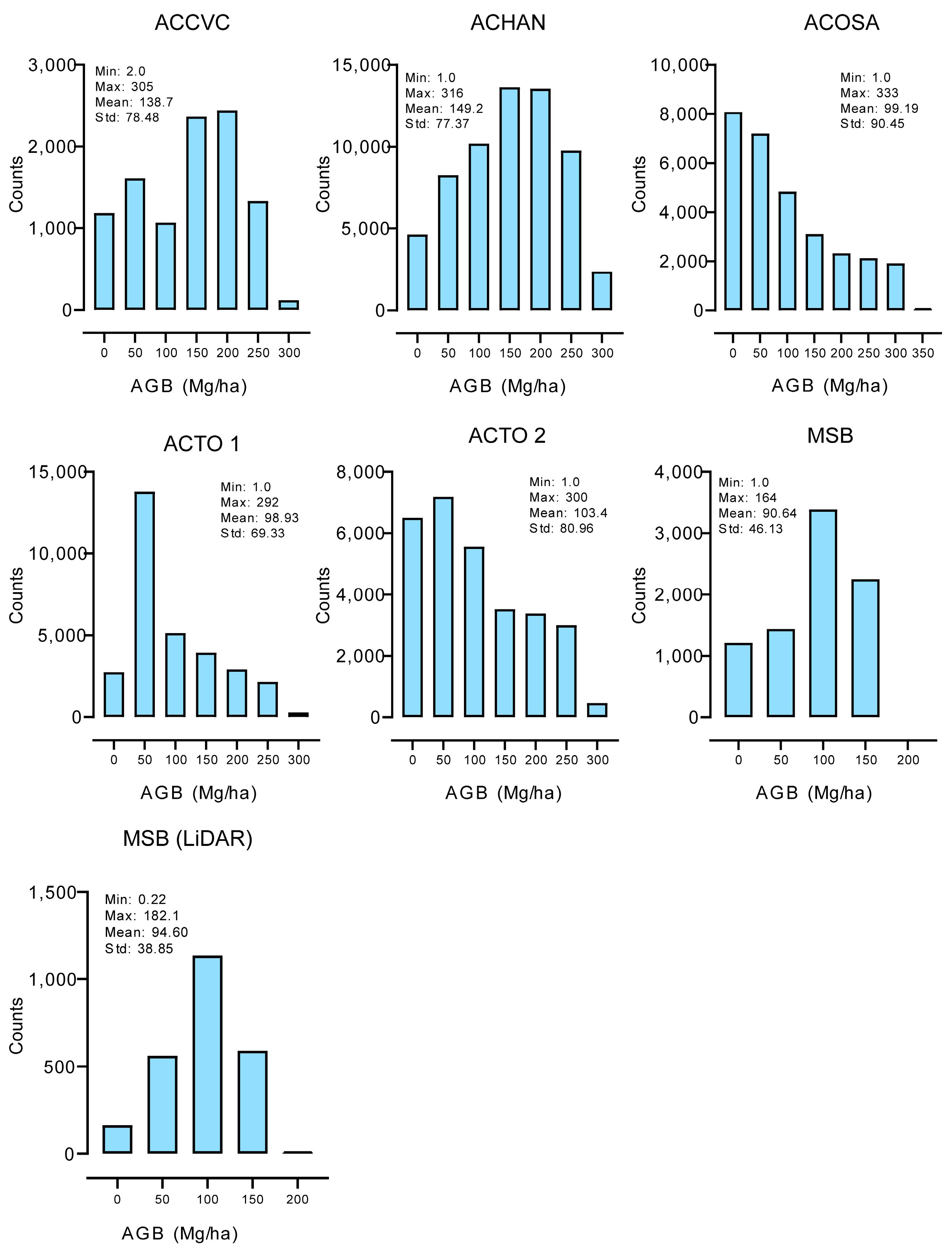
2.1. Study Areas

Our study was carried out in four conservation areas in Costa Rica and one in Canada, with a combined spatial area of approximately 176,332 ha (

Table 1. Characteristics of the tropical and temperate forest ecosystems where hyperspectral imaging data were acquired for this study in Costa Rica and Canada. The elevation presented is the mean with one standard deviation.

Region of Interest	Conservation Area	Forest Type	Precipitation (mm/Year)/Elevation (m)	Total Area (ha)	Total Flight Lines
ACCVC	Area de Conservacion Cordillera Volcanica Central	Tropical wet	4000–8000/206 ± 182	50,251	32
ACHAN	Area de Conservacion Huetar Norte	Premontane wet	4000–8000/117 ± 44	11,989	5
ACOSA	Area de Conservacion Osa	Tropical wet	4000–8000/100 ± 119	67,959	16
ACTO	Area de Conservacion Tortuguero	Tropical wet	4000–8000/41 ± 39	45,177	15
MSB	Mont Saint Bruno National Park	Temperate	50–1300/12 ± 9	990	2
			Total	176,336	74

). The conservation areas in Costa Rica can be classified as tropical wet or moist forests, according to Holdridge Life Zones [51,52]. The forest in Mont Saint Bruno (MSB) National Park is classified as a predominantly deciduous, northern temperate forest [53].

2.2. Hyperspectral Imagery

Airborne HSI was acquired in Costa Rica for the Mission Airborne Carbon 2013 (MAC13) project in April 2013 with two pushbroom systems, the Compact Airborne Spectrographic Imager (CASI-1500), hereafter referred to as CASI, and the Shortwave Airborne Spectrographic Imager (SASI-644), hereafter referred to as SASI [28].

Table 2. Characteristics of the CASI and SASI sensors employed for the MAC13 and CABO projects’ data acquisition. The SASI-644 was used for MAC13 which the SASI-640 was used for CABO.

Sensor Characteristics	CASI-1500	SASI-644	SASI-600
Field of view (°)	39.9	39.7	39.7
No. of across-track pixels	1493	640	600
No. of spectral channels	288 (max) (programmable)	160 (non-programmable)	100 (non-programmable)
Spectral range (nm)	375–1050	883–2523	957–2442
Spectral resolution (nm)	3.2 nm	16 nm at 883 nm and 12 nm at 2523	15 nm

, Tables S1 and S2 describe the sensor characteristics and acquisition parameters of each area. While the CASI sensor records data in the visible and near-infrared portions of the reflective electromagnetic spectrum (375 nm–1050 nm) in up to 288 bands, the SASI records the shortwave infrared (SWIR) region of the electromagnetic spectrum from 883 nm to the 2523 nm in 160 bands. For the flight lines used here, the CASI data were summed spectrally on-chip, resulting in 199 bands.

Through the Canadian Airborne Biodiversity Observatory (CABO) in July 2022, the same CASI, along with a newer SASI-600 SWIR system (Figure 1, Tables S1 and S2), were deployed. This newer SASI has two distinct detectors covering the right and left halves of the flight line, recording spectral information over 100 spectral channels (957–2442 nm).

Both the MAC13 and CABO datasets underwent standard preprocessing routines (Figure S1), including spectroradiometric calibration and geocorrection, using software from the sensor manufacturer, as described in [54,55,56,57]. Atmospheric compensation and topographic and BRDF correction were conducted using the Atmospheric/Topographic Correction for Airborne Imagery (ATCOR 4) program (version 7.3.0 2020) (ReSe Applications GmbH, Wil, Switzerland) following the steps described by [55,56,58]. During geocorrection, the final reflectance product was resampled to 2.5 m pixel size for the MAC13 data and 1 m pixel size for the CABO dataset.

Following the fusion workflow outlined in [59], full range (VINIR–SWIR) reflectance products were generated for all of the study areas. Next, the HSI was spatially resampled to 30 m in ENVI v.5.6.1 (NV5 Geospatial, Broomfield, CO, USA). Subsequently, as described by [56], for the fused imagery, wavelength ranges <400 nm in the visible spectrum, as well as atmospheric water absorption (i.e., wavelength ranges of 1367–1492 nm and 1800–2200 nm) in the SWIR, were excluded from the analysis.

2.3. Training and Field Data

Considering the large training data requirements for machine learning models, in this study, we used an existing AGB dataset as the predominant source of training data for all sites (Section 2.3.1). This training data requirement, more than what is currently available from field data, is necessary for deep learning approaches such as CNNs to avoid overfitting and poor model generalization [49]. Separately, for MSB, we also used airborne LiDAR data for training. Due to their relatively small sample size, field data (Section 2.3.3) were used as a separate validation dataset for our results. Consequently, 2000 virtual plots, each measuring 100 m × 100 m and collectively representing approximately 12% of the total image area, were randomly selected from across the boundary of the ACTO-1 experimental site for training, validation, and testing (Figure S2). The size of these polygons matched the spatial resolution of the global AGB dataset.

2.3.1. Global Above Ground Biomass Map (Tropical and Temperate)

The Global Aboveground Biomass (GAGB) map [60] was used as the primary source of AGB training data for both the tropical and temperate forest sites. This global AGB map was produced for the year 2010 using a combination of C-band synthetic aperture radar data from Sentinel-1 and L-band ALOS-2 in conjunction with some multispectral datasets. It has a spatial resolution of 100 m [60,61]. The GAGB accuracy was assessed to be 58.6 Mg/ha and 44.4 Mg/ha overall RMSE for tropical and temperate forests, respectively [62].

2.3.2. Airborne LiDAR (Temperate Forest)

This study employed discrete multi-return airborne LiDAR previously acquired for the Montérégie region of Quebec, Canada, for the provincial government [63]. The LiDAR data have a point density of approximately 2 points per square meter. The LiDAR point cloud underwent an initial segmentation process to distinguish ground and non-ground points in MATLAB v2023b (Mathworks, Nattick, MA, USA). Subsequently, normalization of the non-ground points was conducted, employing the ground points as a reference before calculating LiDAR metrics such as the 7th decile. To relate the LiDAR metrics to AGB and generate a second independent training dataset, we selected the northern hardwood-mixed wood/deciduous forest model described by [64]. This model relates 7th decile LiDAR height to biomass derived from ground inventory plots to estimate AGB with a reported R² of 0.73 (RMSE of 20.6 Mg/ha).

2.3.3. Field Data

As verification of the applicability of the GAGB dataset, a comparison with independent field data was made for the ACTO-1 conservation area (the least cloudy area from the Costa Rican HSI—Figure 1), and the MSB site in Canada. For ACTO-1, an existing geographic information system (GIS) geodatabase with forest inventory information from Costa Rica’s Natural Forest Management Plans (NFMP) [65] was used. To account for total AGB within a plot, census and tree inventory data from private land holdings were extracted from this database. The census includes trees with a diameter at breast height (DBH) greater than or equal to 60 cm, while the tree inventory data includes all trees in 0.3 ha plots greater than or equal to 30 cm (see [52,65] for details). The polygons of the parcel boundaries were cleaned to avoid duplications, overlaps, and to correct the topology. Parcels with forest loss between the date of the inventory and April 2013 (i.e., acquisition of the HSI data) were also removed. A total of 34 parcels ranging in area from 5 ha to 312 ha remained after data cleaning and quality assurance checks. For these, tree-level AGB was calculated with Equation (1) for the census data using the Brown Equation for tropical wet forests [66]. The estimated biomass for the inventory was then extrapolated to the farm level and added to the census biomass.

Y = 21.297 − 6.953 (D) + 0.740 (D²)

(1)

where D is the DBH.

For MSB, field inventory data from the CABO repository [67] were used for the estimation of AGB. Fifteen field plots (30 m × 30 m) with a minimum of 30 individual trees were inventoried in 2019. For each plot, measurements of every tree within a 15 m radius from a precisely georeferenced and permanently marked plot center were conducted. Every tree with a DBH of <9 cm, whose canopy is visible from above, and all trees with a DBH of ≥9 cm were measured, including the inventory of their height and canopy dimensions using a T3 Transponder and LaserGeo (Haglöf, Sweden AB, Långsele, Sweden) instruments. Each tree was identified to the species level, and a canopy dominance value (dominant, codominant, intermediate, or suppressed) was assigned. To estimate AGB, the trees marked as dominant and codominant were selected, since they are the trees whose canopies are readily mapped by remote sensing. The methods outlined in [68,69] were used to calculate the AGB for each tree stand, and the results were aggregated to the plot level.

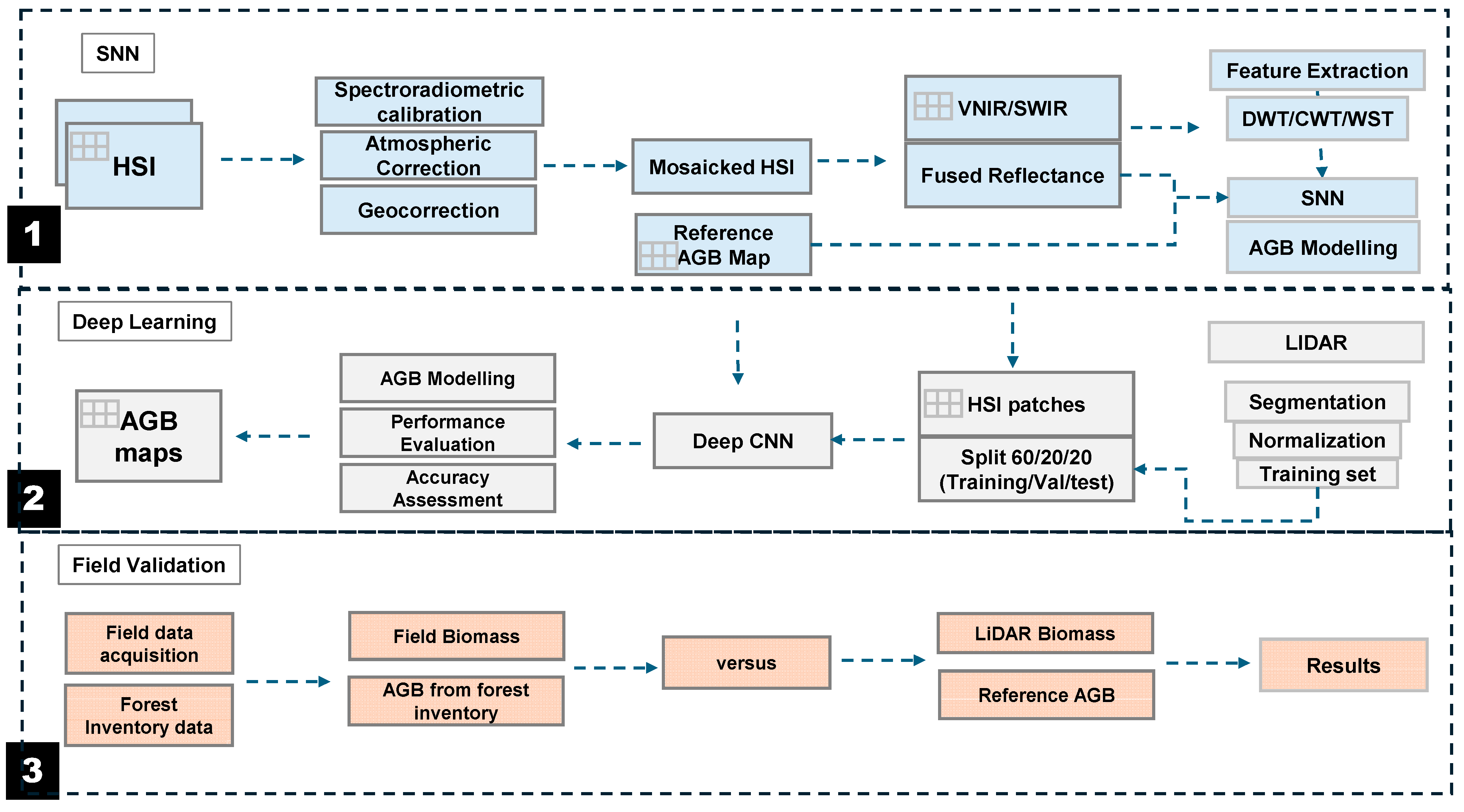
2.4. Machine Learning Model Development and Evaluation

To compare the output of different machine learning approaches and wavelet transformations, the ACTO-1 conservation area was selected as a proof-of-concept test site. The model type with the lowest RMSE was then independently developed for the remaining tropical forest sites and MSB. As summarized in Figure 2, three types of wavelet transformations (i.e., continuous wavelet transform—CWT, discrete wavelet transform—DWT, and wavelet scattering transform—WST) were tested along with two neural networks (i.e., shallow neural networks—SNN and 3D deep convolutional neural networks—3D-CNN). The objective is to compare the performance of these two distinct methods—wavelet transforms combined with SNN and 3D-CNN. As described below, the first method utilizes wavelet coefficients at different scales as features, which are then used to train the SNN. This approach leverages the multiresolution capabilities of wavelets and the simplicity of shallow networks, ensuring computational efficiency for smaller datasets. The second method directly inputs spectral images into a 3D-CNN model, treating each pixel as a 3D data cube with multiple spectral bands. The 3D-CNN extracts spatial and spectral features by analyzing data across three dimensions, making it highly effective for complex datasets. A brief description of these methods is presented below.

2.4.1. Wavelet Decomposition

A wavelet is a waveform of limited duration used to decompose a signal (e.g., spectrum) into shifted and scaled representations of the original waveform (i.e., the mother wavelet), which is equivalent to increasing levels of spectral details or radiant frequencies [70]. Wavelet decomposition permits the simultaneous analysis of the reflectance spectra in the time and frequency domains [71,72]. The two main types of wavelet transforms explored in this study are continuous (CWT) and discrete (DWT). These two wavelet types differ in how they both discretize the scale and translational (or shifting) parameters of the mother wavelet. While the DWT uses a finite set of scales (subset of scales and positions) known as discrete dyadic scales, where scales are on the order of the power of 2 [73], the CWT can operate at every scale and includes the scale as determined from the input signal to a scale specified by the user.

The set of wavelet basis functions is computed for the input signal by shifting and scaling ψ(λ), which is known as the mother wavelet, across the signal (Equation (2)), as follows:

$${\psi }_{a,b}\left(\lambda \right)={\displaystyle \frac{1}{\sqrt{a}}}\psi \left({\displaystyle \frac{\lambda -b}{a}}\right)a>0,b\in ℝ$$

(2)

where a is the scaling factor and b is the shifting factor.

The calculated coefficients for the shifting and scaling factors constitute the sum of the multiplication of the reflectance spectrum across all wavelengths by the scaled and shifted representations of the mother wavelet. For the CWT, Morse, bump, and Morlet mother wavelets were chosen for comparison, while, for the DWT, two mother wavelets from the Daubechies family (db6 and db5) and a symlet wavelet (sym7) were chosen based on [74].

In addition to DWT and CWT, we also tested a wavelet scattering transform (WST) to extract spectral features for AGB modeling. The WST extracts informative spectral features with low variance and stable representation of the reflectance data. The method applies wavelets and scaling functions to reflectance data to extract features that can be packaged as inputs for deep learning and other machine learning applications. The steps in WSTs include convolution applied to the input spectrum using wavelets (i.e., Gabor and Morlet wavelets were tested), followed by non-linearization and averaging (pooling) using scaling functions. Three scattering networks (WST-N1, WST-N2, and WST-N3) were tested to determine the appropriate sampling frequency that would maximize the information content. Sampling frequencies of 20, 30, and 50 were used to produce scattering coefficients with lengths of 60, 30, and 15, respectively.

2.4.2. Spectral Feature Selection

After transforming each spectrum using the DWT, CWT, and WST, as demonstrated by [75], the correlation coefficient between AGB and the coefficients at various levels of decomposition was calculated per wavelet transform to select robust spectral features. Considering the variability of the number of coefficients at various levels of decomposition for each wavelet type, we selected a different threshold for each wavelet type that would produce features not exceeding 250 for the modeling. Several runs were conducted to identify the optimal thresholds for determining robust spectral features for AGB modeling. This involved including preliminary models with varying thresholds and evaluating their performance based on criteria such as model accuracy and computational efficiency. For instance, for the DWT and CWT, thresholds of 0.45 and 0.6 were selected, respectively. For the WST, except for WST-3, where a threshold of 0.2 was applied, no threshold was applied for WST-1 and WST-2 since the produced features were within the set feature limit.

Additionally, mutual information feature selection was used to rank the spectral features. This method captures linear and non-linear relationships in datasets [76]. The spectral features within the set limit, as mentioned above, were subsequently used for AGB modeling, and their modeling performance was compared with the threshold-based feature selection described above.

2.4.3. Shallow Neural Network (SNN)

A typical artificial neural network (ANN) architecture comprises the following three main components: an input layer, hidden layer, and output layer (Figure S3) [77]. For the ACTO-1 conservation area, the selected spectral features from the wavelet coefficients were used to train a two-layer feed-forward SNN with ten sigmoid hidden neurons in the first layer and an output linear neuron with MATLAB 2021b. The network was trained using the Levenberg–Marquardt back-propagation training algorithm. A total of 60% of the training data was randomly assigned for training, with 20% used for validation and the remaining 20% for testing. The weights and biases of the SNN were adjusted using the selected training data to help to predict the dependent variable (AGB) from the selected spectral features. The generalization ability of the model was then evaluated based on its performance on the validation and test sets. For instance, during training, overfitting of the model was avoided by stopping the learning process early using the outcome from the validation data (i.e., if no improvement in the validation error was observed in successive epochs). Meanwhile, the test set served as an independent validation of the generalization abilities of the model.

2.4.4. Deep Transfer Convolutional Neural Network Framework (3D-CNN)

A three-dimensional convolutional neural network (3D-CNN) is a type of neural network designed to analyze a three-dimensional dataset like HSI. Hyperspectral data cubes comprise two spatial dimensions (i.e., X and Y) and a spectral dimension. The high dimensionality of HSI results in high computational complexity when a 3D-CNN model is employed to extract spectral–spatial features for regression or classification. Therefore, to improve the efficiency of 3D-CNN implementation and reduce spectral correlation and noise while preserving the spectral information content, a Principal Component Analysis (PCA), Maximum Noise Fraction Transform (MNF), and t-Distributed Stochastic Neighbor Embedding (t-SNE) were implemented on the HSI before employing the 3D-CNN to extract spectral–spatial features for modeling AGB [47], and their results were compared. Figure S4 shows a subset of the HSI from ACTO-1 with dimensions of 190 columns × 163 rows × 238 bands. After implementing a PCA or MNF, the spectral bands are reduced to the first 15 components. For the t-SNE, three components remained. Next, each pixel vector was assigned a corresponding AGB value extracted from the GAGB reference map or LiDAR. Blocks of pixels representing a 3D patch from the HSI and centering on each pixel were created from adjacent pixels with a stride of 1 to produce a patch with dimensions of m × m × P. Here, m × m is the window size used for splitting the imagery into 3D patches, and P is the number of bands following PCA, MNF, or t-SNE. The output of the spectral–spatial feature extraction using the 3D-CNN is produced by applying a 3D convolution three times, each followed by a Rectified linear Unit (ReLU), an activation function that introduces non-linearity in the output of the network, with the last one followed by max-pooling and a flattened layer. These flattened layers are also followed by a dropout layer (i.e., a regularization technique). Figure S5 shows the model architecture. The model is based on the architecture shown in [78]. Multiple splits were tested through several runs and analyses, and data splits of 60% for training, 20% for validation, and 20% for testing were found to be sufficient to ensure model generalization. To mitigate overfitting, regularization methods such as dropout layers, weight decay, and early stopping based on the performance of the 20% unseen validation data were employed. In summary, the inclusion of max-pooling in the deep learning architecture, a reduced training time for the model (i.e., 40 epochs), the utilization of 30% and 20% dropout rates, a window size of 15 for extracting spatial and spectral features, and a split ratio of 60:20:20 for training, validation, and testing were key measures implemented to help avoid overfitting and improve model generalization.

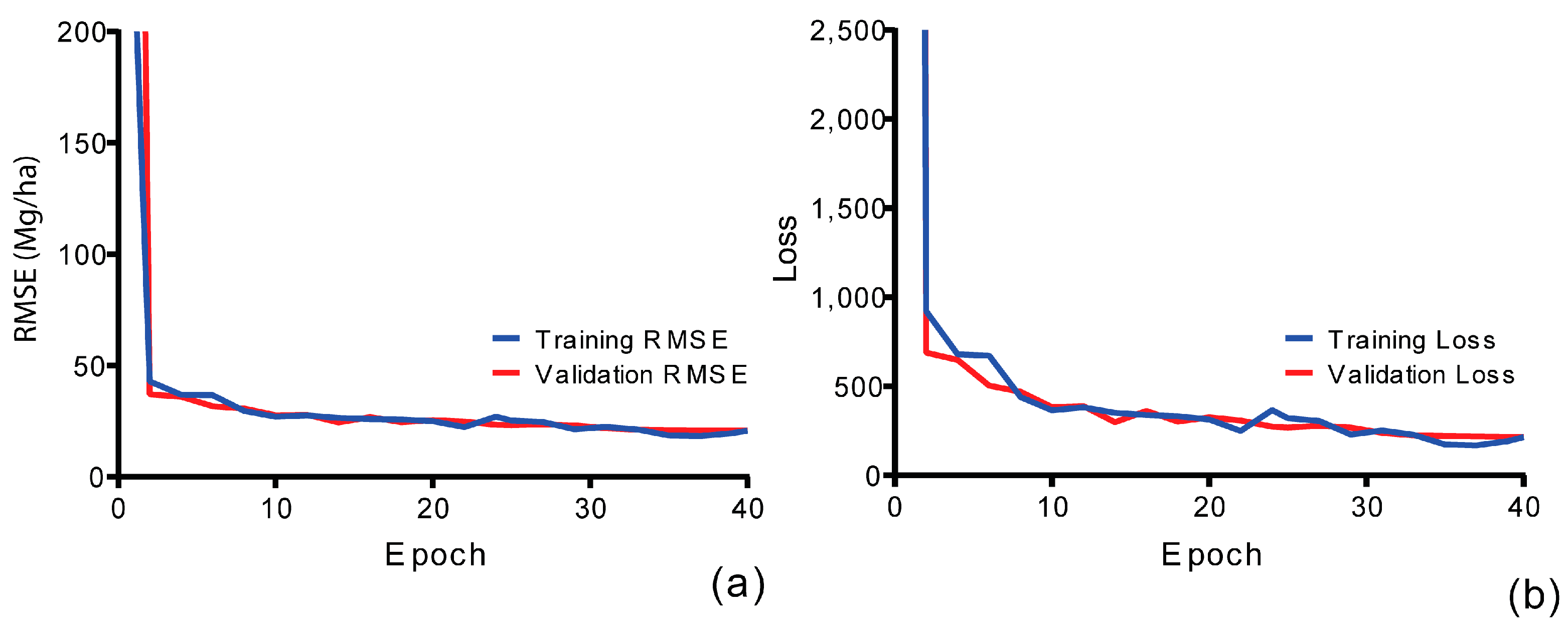
2.4.5. Hyperparameter Tuning

The process of optimizing or tuning parameters such as batch size, number of epochs, number of hidden layers, learning rate, and the dropout parameter is known as hyperparameter tuning, which was performed using MATLAB 2023b for the SNN and 3D-CNN models (

Table 3. Hyperparameters employed in the SNR and 3D-CNN models. The hyperparameters were selected by running several tests and analyzing the results.

	Epochs	Minibatch Size	Optimizer	Learning Rate	Loss Function
SNN	1000	-	Levenberg M	0.1	MSE
CNN-3D	40	256	Adam	0.001	RMSE

). We employed a learning rate of 0.1, which is frequently used for the Levenberg–Marquardt algorithm, and 0.001, which is also commonly employed for the Adam optimizer.

2.4.6. Performance Metrics for Model Evaluation

The models’ performances were evaluated per network architecture (SNN and 3D-CNN), as well as the input data/wavelet type. We selected three main metrics frequently used in the literature to assess the performance of the models. These metrics were the mean square error (MSE), root mean square error (RMSE), and mean absolute error (MAE). To compare the differences between the GAGB map pixels (and LiDAR-based AGB at MSB) and the predicted AGB map, an AGB bin of 40 Mg/ha was selected, and the predicted values were tabulated and graphed based on this bin versus the corresponding GAGB (or LiDAR-based) values. Two main accuracy metrics, namely the root mean square difference (RMSD) and mean difference (MD), which can be referred to as the bias, were used to assess the accuracy of each model. The RMSD was calculated according to Equation (3), as follows [79]:

$$RMSD=\sqrt{{\displaystyle \sum }_{j=1}^n{\displaystyle \frac{{\left(AG{B}_{Pm}\left(i\right)-AG{B}_{Refm}\left(i\right)\right)}^2}{n}}}$$

(3)

where AGB_Pm is the predicted aboveground biomass, AGB_Refm is the reference aboveground biomass (i.e., GAGB- or LiDAR-based AGB), and n is total number of observations.

The mean difference was calculated according to Equation (4) as follows:

$$MD=\left(\mu AG{B}_{Pm}-\mu AG{B}_{GAGBm}\right)$$

(4)

where μAGB represents the mean aboveground biomass.

2.5. Proof-of-Concept Model Development

As mentioned in Section 2.4, to compare the output of the SNN (with different wavelet transformations) and the 3D-CNN, the ACTO-1 conservation area was selected as a proof-of-concept test site. To set up the input data, firstly, 2000 virtual plots (100 m × 100 m) were randomly distributed across ACTO-1. The area of these plots is equivalent to the pixel size of the GAGB dataset, and the GAGB values for each plot were assigned to the polygons. For both the SNN and the 3D-CNN, pixels were extracted from the HSI for the 2000 plots and used as training samples, which constituted approximately 22,000 pixels. The samples were split into 60% for training (n = 13,200), 20% for validation (n = 4400), and 20% for testing (n = 4400). The range of the GAGB-based AGB values was 0–300 Mg/ha (μ = 150.1 ± 86.5 Mg/ha).

2.6. Aboveground Biomass Modeling in Different Forest Types

Development of AGB models based on forest type is recommended to account for the variability of the forest types and spectral characteristics [80], therefore, a separate 3D-CNN model following the architecture described in Section 2.4.4 was developed for each of the other Costa Rican sites (i.e., ACHAN, ACOSA, and ACCVC) and for MSB in Canada. At MSB, a 3D-CNN model was also developed using the LiDAR-based input data (see Section 2.3.2). Summary statistics of the reference GAGB (and LiDAR-based AGB for MSB) data are shown in Figure 3.

3. Results

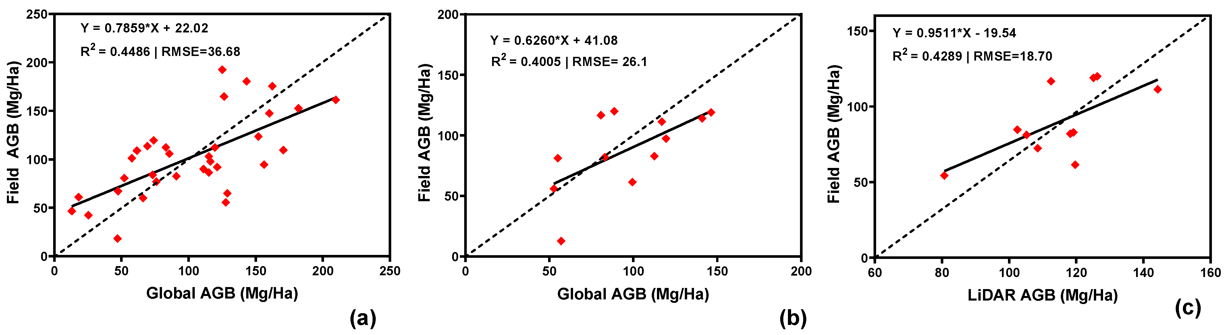
3.1. Comparison of Training Data with Field-Based AGB

The results comparing forest inventory estimates of AGB and the reference GAGB data used for training are shown in Figure 4. For both tropical and temperate forests, a moderate relationship can be seen. For ACTO-1, an RMSE and R² of 36.68 Mg/ha and 0.45, respectively, were found, while, for the temperate forest (MSB), an RMSE of 26.1 Mg/ha and an R² of 0.40 were found (Figure 4). The comparison between the estimated field AGB and the LiDAR-based AGB estimates for MSB resulted in an RMSE of 19.54 Mg/ha and an R² of 0.42 (Figure 4).

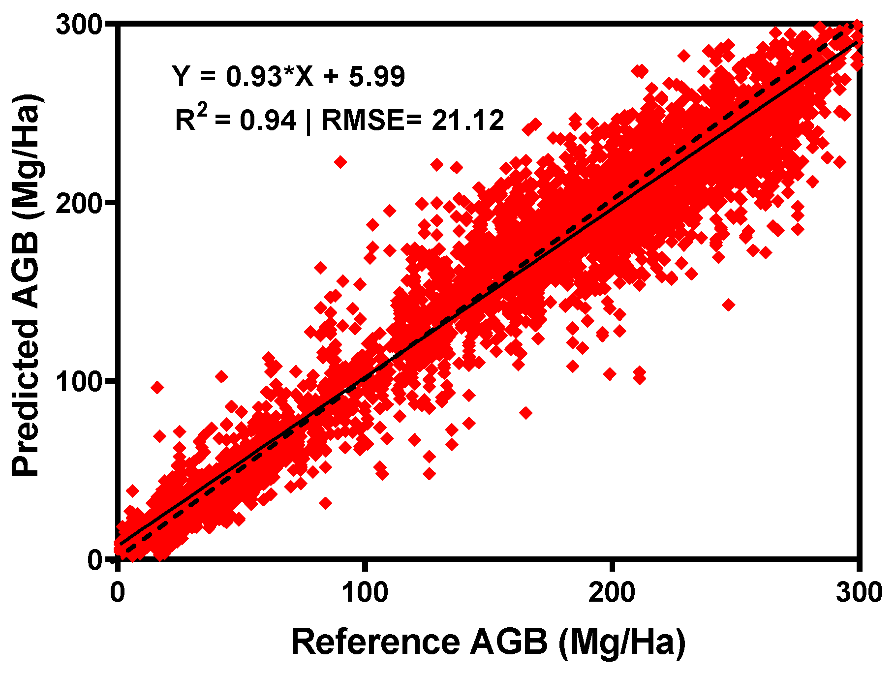
3.2. Proof-of-Concept Model Comparison

3.2.1. SNN Model Comparisons

For the ACTO-1 conservation area proof-of-concept model development, the results of 20 iterations of the SNN model for each type of wavelet transform are presented in

Table 4. Shallow neural network model comparisons across wavelet decomposition inputs with results ordered by RMSE (best to worse). Units for RMSE, MSE, and MAE are in Mg/ha. The average is based on 20 iterations.

Input Variable	# Extracted Features	Performance	MSE	MAE	R	R2	RMSE
DWT-db6	225	Best Model	2032.36	34.97	0.85	0.72	45.08
		Average	2132.71	35.88	0.85	0.72	46.17
WST-N3	199	Best Model	2039.68	34.66	0.85	0.72	45.16
		Average	2159.49	35.92	0.84	0.71	46.46
WST-N2	210	Best Model	2050.8	35.09	0.85	0.72	45.29
		Average	2241.14	36.73	0.84	0.71	47.33
WST-N1	135	Best Model	2071.35	35.06	0.85	0.72	45.51
		Average	2266.27	36.9	0.84	0.71	47.6
DWT–sym7	203	Best Model	2123.02	35.55	0.85	0.72	46.08
		Average	2266.12	36.86	0.83	0.69	47.58
DWT–db5	213	Best Model	2158.07	36.01	0.84	0.71	46.46
		Average	2274.16	37.04	0.83	0.69	47.68
CWT–bump	35	Best Model	3308.62	44.35	0.75	0.56	57.52
		Average	3503.86	45.7	0.73	0.53	59.19
CWT–amor	119	Best Model	3530.41	45.95	0.73	0.53	59.42
		Average	3688.4	47	0.71	0.5	60.73
CWT–morse	79	Best Model	3531.01	46.07	0.73	0.53	59.42
		Average	3823.43	47.04	0.70	0.49	61.7

. Across the wavelet decomposition types, the CWT resulted in the highest RMSE, ranging from 57.52 Mg/ha to 79.23 Mg/ha for the threshold-based feature selection and 49.66 Mg/ha to 57.63 Mg/ha for the mutual-information-based feature selection. The best CWT model was found to be with the bump wavelet, which resulted in an RMSE of 49.66 Mg/ha. In contrast, the results for the DWT and WST are similar in the range of RMSE across all combinations and produced lower RMSE values than the CWT, ranging from 43.478 Mg/ha to 52.02 Mg/ha. For instance, the model derived from DWT-db6 features improved the AGB prediction by approximately 6.2 Mg/ ha compared to the best CWT model. Similarly, all three WST models showed an improvement of model performance by 6 Mg/ha compared to the best CWT model with the best WST models, achieving an RMSE of ~44 Mg/ha (Table 4 and Table S4).

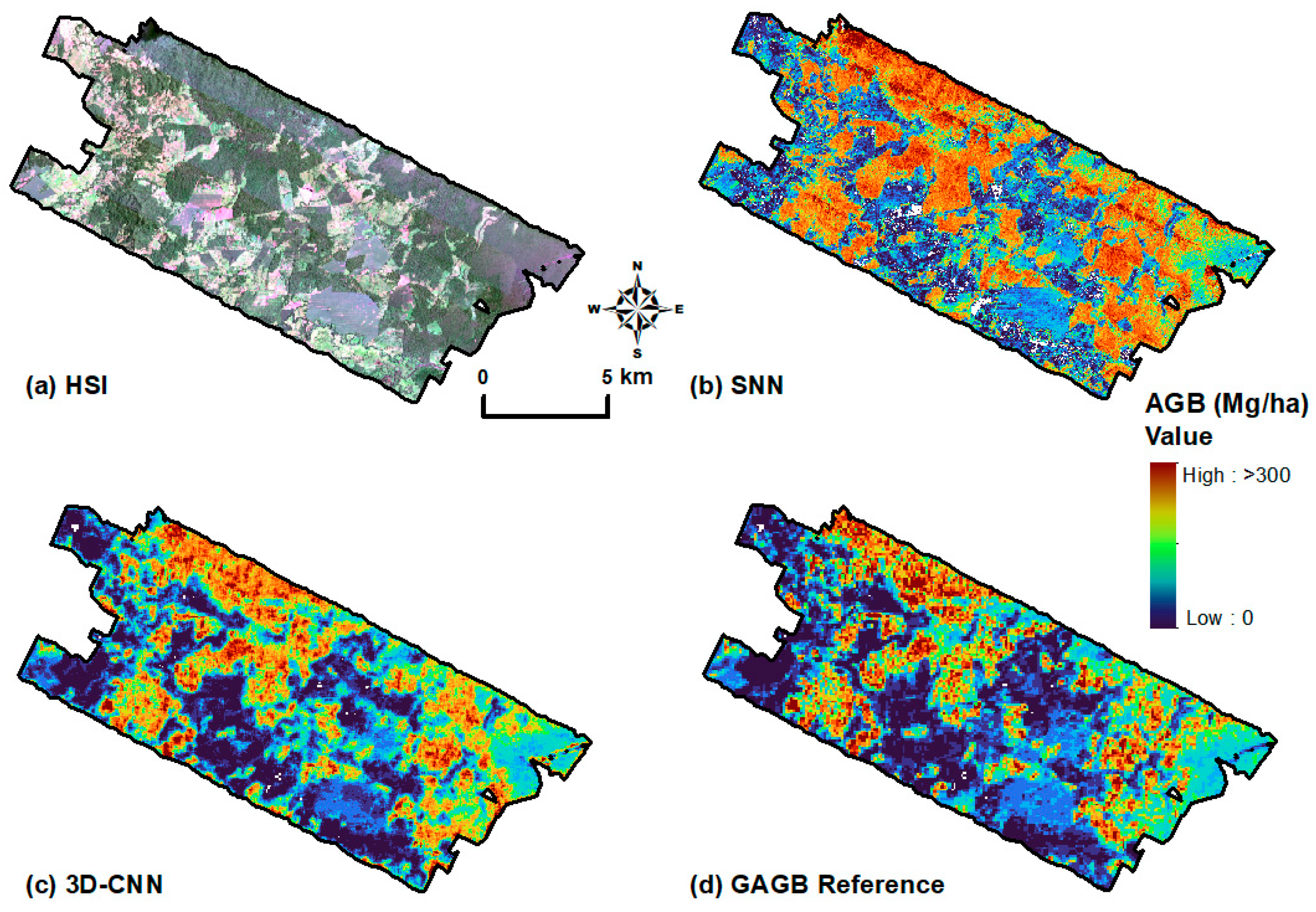
3.2.2. Spectral–Spatial Features (3D-CNN)

Extracting spatial information along with spectral information for AGB modeling using the PCA-based 3D-CNN resulted in a low RMSE of 21.12 Mg/ha and an R² of 0.94 compared to an R² range of 0.8–0.92 and RMSE values of 24.15–35.92 Mg/ha for the MNF- and t-SNE-based 3D-CNN (Figure 5 and

Table 5. A comparison of 3D-CNN-based AGB modeling performances for different HSI dimensionality reduction approaches.

	PCA	MNF	t-SNE
R square	0.94	0.92	0.83
RMSE (Mg/ha)	21.1	24.15	35.92

). The results for the 3D-CNN models represent the lowest RMSE values compared to the SNN approach, which relies on spectral features alone (Table 4 and Table 5). Figure 6 presents the 3D-CNN learning curve, showing the training and validation RMSE and loss for PCA-based 3D-CNN AGB modeling. From Figure 6, it can be deduced that convergence was reached after approximately the 10th epoch, where the training RMSE and loss tends to become stable (Figure 6a,b).

Additionally, Figure 7 shows a predicted AGB map derived from the best SNN-WST-N3 model developed at the ACTO-1 experimental site and the PCA-based 3D-CNN model at the landscape scale for the same site. In comparison to the reference GAGB map, the landscape-scale SNN-WST-N3 model resulted in an R² of 0.72, while the 3D-CNN model based on PCA performed better, resulting in an R² of 0.94. Given the split ratio of 60:20:20 for training, validation (seen), and testing (unseen) data in the AGB modeling, a comparison between the results of the validation and testing sets revealed no significant performance drop. For instance, the final validation RMSE achieved was 20.83 with an R² of 0.941 for the validation set (Figure 6a). Meanwhile, using the test set (unseen data), the final validation RMSE resulted in 21.12 Mg/ha with an R² of 0.939 (Table 5 and Figure 5). A summary of a comparison of the results with or without PCA methods is presented in Table 5 and Figures S7 and S8.

3.3. Benchmark Dataset Comparison

When the 3D-CNN model developed for the ACTO-1 site (experimental site) is applied to imagery of the same forest type in a nearby location (ACTO-2) and compared to the reference GAGB, the results show an R² of 0.62 (Figure S6a). A drop of approximately 0.3 in the R-squared values between the results for the ACTO-1 experimental site model (R²~0.9) and that of the ACTO-2 benchmark site (R²~0.6) was recorded, indicating a correlation of 0.77 between the reference and the prediction (Figure S6). Similarly, a drop of 0.3 in R² was observed when the SNN model for ACTO-1 was applied to the ACTO-2 site, recording an R² of 0.40 (Figure S6b).

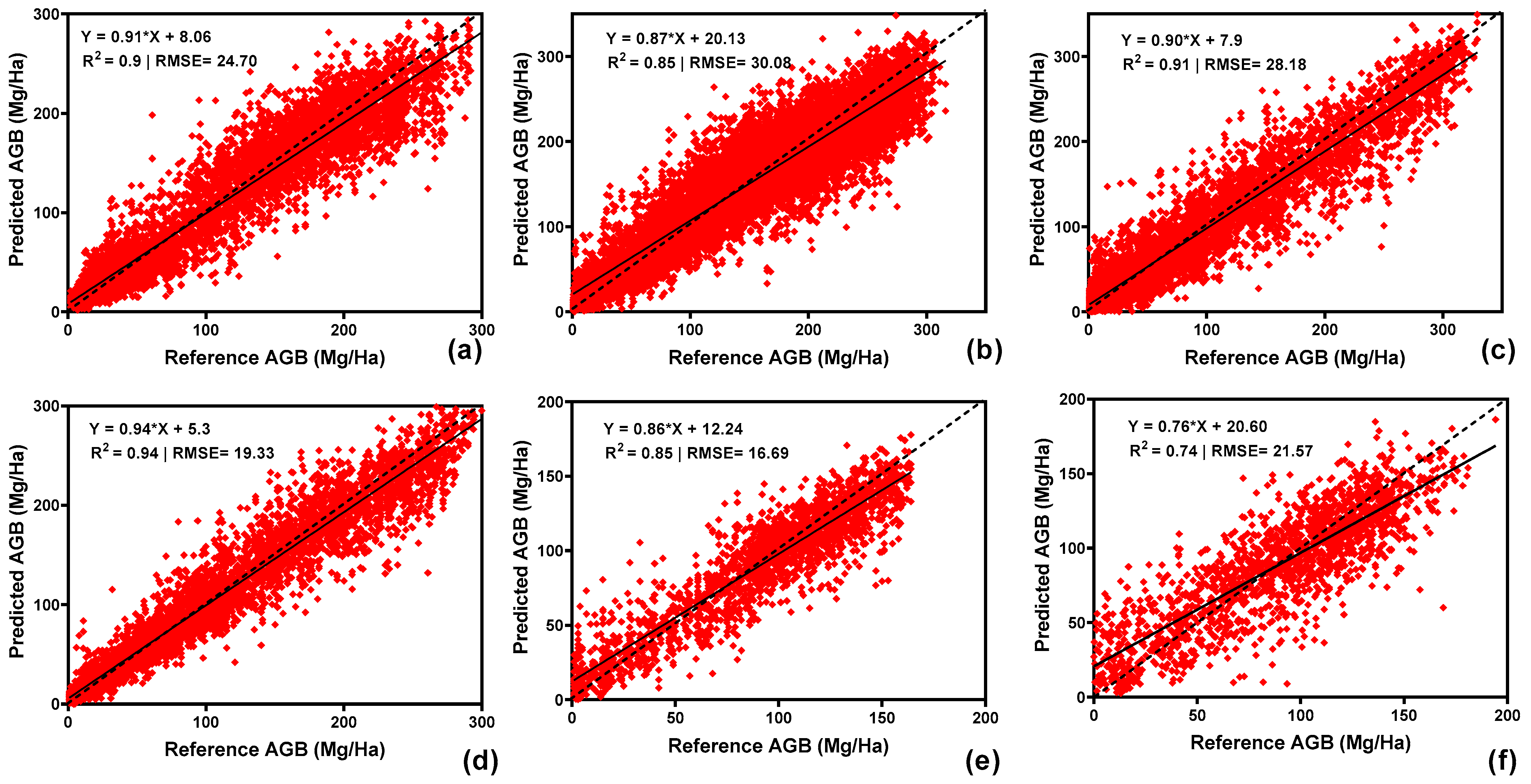
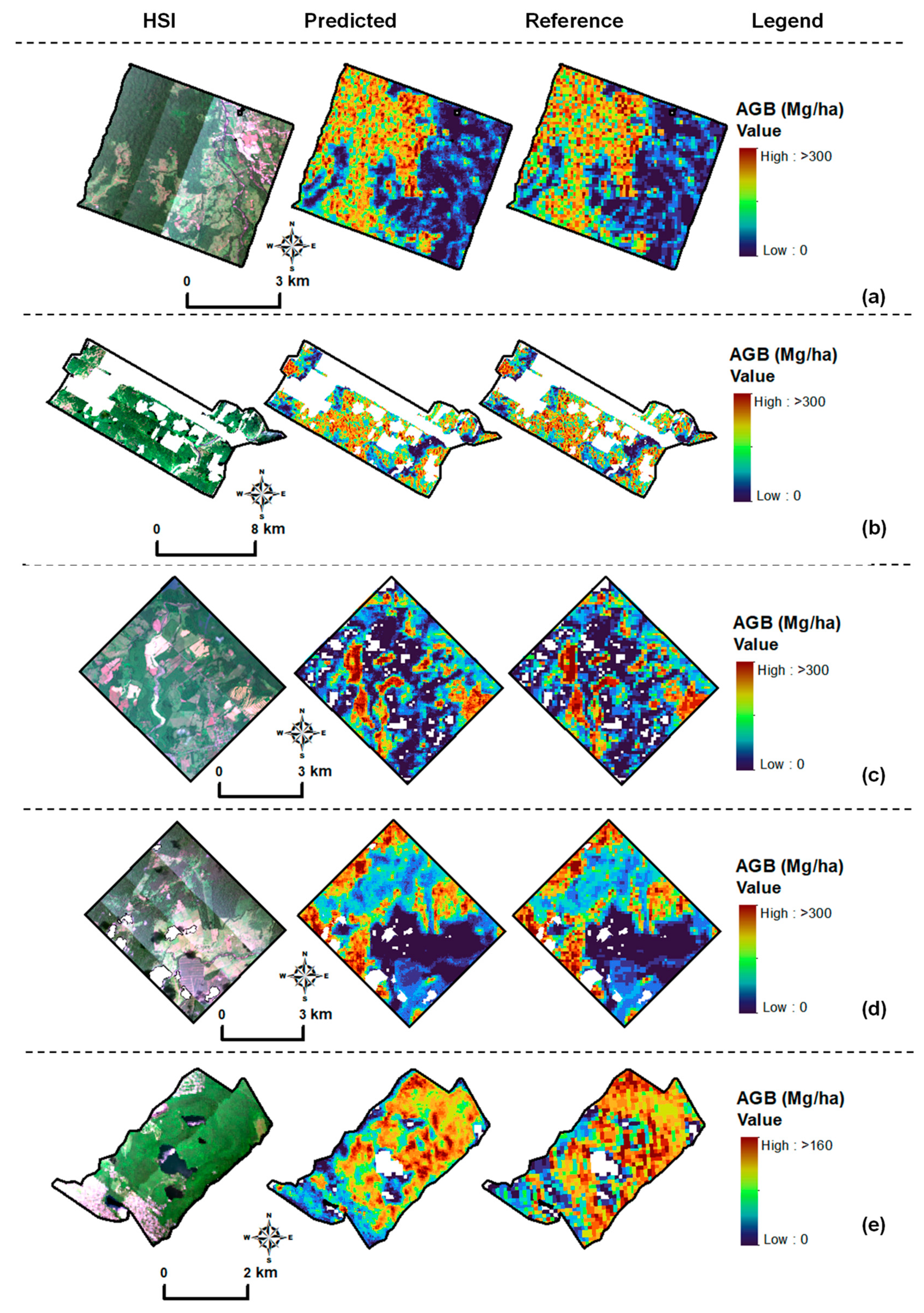
3.4. Model Performance Across Forest Types (Hyperspectral Imagery)

The summary results of the development of a PCA-based 3D-CNN (best performing model type at the test site) for each forest type are presented in Figure 8. While the lowest RMSE can be seen for MSB (16.69 Mg/ha), all forest types have similar results with RMSE, ranging from 24.70 Mg/ha (ACCVC) to 30.1 Mg/ha (ACAHN). Applications of the 3D-CNN models at the landscape scale for each forest type are shown in Figure 9. The figure shows that, apart from ACHAN, the tropical wet forests ACCVC, ACOSA, and ACTO produced the best model performance, with an RMSE in the range between 19 and 28 Mg/ha. Compared to the tropical forests, the predicted AGB range was the lowest at MSB (temperate forest), with a minimum and maximum of 0 and 176 Mg/ha, respectively.

A plot of the biases of selected AGB bins showing which range of AGB was under- or overpredicted is shown in Figure 10, and a tabulation of the results for the selected accuracy metrics (RMSD and MD) are also presented in Table S3. Overall, it can be deduced that the predicted AGB values were closely related to those of the reference map. For instance, Figure 10 shows that, for all of the tropical forests, apart from ACOSA, AGB values within the range of 0–280 were underpredicted up to 5 Mg/ha, while the AGB greater than 280 Mg/ha were overestimated up to about 20 Mg/ha. At ACOSA, AGB was underpredicted up to about 10 Mg/ha and overpredicted up to approximately 5 Mg/ha. However, MSB recorded the lowest underprediction of the AGB values within the range of 0–160 Mg/ha (4 Mg/ha) but overpredicted up to 6 Mg/ha for the AGB values above 160 Mg/ha. Moreover, Table S3 shows that the highest RMSD values (19.0 Mg/ha–25.4 Mg/ha) for all of the tropical forests were found to be for the AGB range of 160–200 Mg/ha, and the lowest RMSD was recorded for the 0–40 Mg/ha range. Similarly, for MSB, the lowest RMSD (~15 Mg/ha) was recorded for the AGB range of 0–40 and the highest (16–21 Mg/ha) was recorded for the AGB range of above 40 Mg/ha.

3.5. Model Performance—Airborne LiDAR

The results of a 3D-CNN model based on the airborne LiDAR data as an input for the MSB site showed an RMSE of 21.57 Mg/ha (R² = 0.74). Figure 11 shows the spatial variability in AGB values for both the reference and predicted AGB of the MSB site. In comparison to the model using the GAGB data, there was a drop in model performance from an R² of 0.85 to 0.74, representing an approximately 13% drop in model performance.

4. Discussion

Large training datasets are crucial in AGB modeling, as they capture heterogeneity, help improve accuracy, enhance generalization, and increase model robustness [48,49,50]. In this study, we demonstrate that, when sufficient training datasets are available for deep learning, 3D-CNN can be used to extract spectral and spatial features simultaneously from HSI to model AGB for improved modeling performance in tropical and temperate forest ecosystems. While other studies have demonstrated the use of 3D-CNN for classification and related tasks (e.g., [47]), our study is the first to show that, with large datasets (i.e., those that are comprehensive and diverse enough), 3D-CNN can achieve a low RMSE in modeling AGB in these ecosystems.

As shown in Figure 4, field-based AGB estimates and the GAGB data (and LiDAR for MSB) have moderate relationships of R² of 0.4–0.44 and RMSE of 18.7–36.7. While they indicate that the GAGB is reasonable in our study areas, those results should be interpreted with caution, as the sample size is small (n = 13–34). The need for, but also the challenges in, establishing large numbers of field plots for forest characteristics such as AGB have been reiterated by many studies, e.g., [81,82,83,84]. There is a large training data requirement for ML approaches to ensure that overfitting is avoided and that the model can generalize well to unseen pixels in the imagery [48,49]. Moreover, as stated earlier, the RMSE of the GAGB dataset is 58.6 Mg/ha and 44.4 Mg/ha for tropical and temperate forests, respectively. While our results show lower RMSE in comparison to the GAGB dataset, it remains a proxy for field data. Therefore, it is important that the overall uncertainty in comparison to ground-based estimates needs to consider not only the uncertainty from our model results, but those from within the GAGB dataset as well. Nonetheless, the 3D-CNN employed in this study has shown promise. As larger field-based datasets become available (i.e., those large enough for the methods employed in this study), the 3D-CNN approach is expected to offer a robust modeling alternative, advancing machine-learning-based approaches to AGB modeling using HSI.

Previous studies (e.g., [85,86,87]) have shown improved model predictive power of vegetation characteristics and classification from wavelet decomposition of HSI over other approaches, including vegetation indices and PCA. Our proof-of-concept model comparison from the ACTO-1 study area compared SNNs with different wavelet decompositions as inputs with a deep learning 3D-CNN. We found that the best wavelet decomposition SNN model was the DWT (db6), with an RMSE of 43.47 Mg/ha. However, our results ultimately showed that the best performing model was the PCA-based 3D-CNN, with an RMSE of 21.12 Mg/ha (Figure 5). This was an improvement in RMSE of 22.35 Mg/ha over the best SNN model, which relies only on spectral features. While the R² values are not comparable between studies, our RMSE range of 21.12 Mg/ha to 30.1 Mg/ha across the forest types is lower than those reported by others, such as [88] (~68.11 Mg/ha), [89] (~91.2 Mg/ha), and [19] (~64.4 Mg/ha), employing individual hyperspectral bands or vegetation indices calculated from HSI. In terms of R-squared values, the use of spectral features from optical imagery and other datasets has shown promising results in estimating AGB, with R² values ranging from 0.84 to 0.92, compared to an R² of 0.5 to 0.68 when hyperspectral features are used alone [29,35,38]. For instance, ref. [90] reported that when temporal features extracted from multiple satellite imagery are used for AGB modeling, an R² of 0.58 can be attained. Spectral metrics, such as vegetation indices extracted from HSI for AGB prediction, also produced an R² of 0.55 in a study conducted by [38]. It has also been reported that the use vegetation indices alone from HSI for AGB prediction in the Brazilian Amazon resulted in an R² of 0.58 [88]. Similarly, [35] reported a moderate relationship (R² ranging between 0.56 and 0.65) for tree- and plot-level AGB estimates. Even in the absence of LiDAR, the results obtained in this study were promising (R² of 0.94 and an RMSE of 21.12 Mg/ha) and comparable to the results obtained in previous studies that employed both optical imagery and LiDAR (e.g., [88]).

By extracting both spectral and spatial information for AGB modeling, our results showed a reduction in AGB prediction uncertainties of the model that relies only on spectral features by ~50% (Figure 5 and Table S4 and Table 4). Using a random forest model to predict tropical forest carbon from LiDAR, ref. [91] also found that a model considering the spatial context performed best. However, the inclusion of the spatial context is not without challenges. The extraction of spatial features simultaneously with spectral features requires a neighborhood of pixels (in this case, 15 × 15 equivalent to ~20 ha). For such a window size (or larger), where high AGB pixels are found among low AGB pixels, less accurate prediction is expected. This also applies to edge pixels and areas transitioning into low-AGB areas (Figure 7c,d). From a flight planning perspective, future studies that employ a 3D-CNN model with airborne HSI should consider the issue of edge pixels to ensure that a sufficient area is covered outside of the area of interest to account for the planned neighborhood window size. Future studies may explore using different kernel sizes to better align with the spatial and spectral characteristics of the imaging data. Misaligned kernel sizes could lead to inefficient feature extraction, causing important patterns to be overlooked. Experimenting with kernel sizes tailored to the spatial and spectral resolutions of the data is usually recommended. In other words, future studies can employ separate kernel sizes for spatial dimensions (height and width) and the spectral dimension (depth) to capture relevant features more effectively. When resizing the spatial dimensions, proportional scaling must be ensured to preserve the original aspect ratio (e.g., resizing to 18 × 15 instead of 15 × 15).

The spatial autocorrelation unaccounted for during the training and validation of a model can result in an overly optimistic modeling performance [92]. In the benchmark data comparison, where the ACTO-1 model was applied to the ACTO-2 imagery, the best performing model had a decrease of 0.3 in the R-square values and an increase in RMSE of 35.83 Mg/ha (Section 3.3 and Figure S6). This drop can potentially be attributed to spatial autocorrelation affecting the model’s generalization. Spatial autocorrelation is known to cause an overestimation of CNN model performance, owing to the potential proximity of the test set pixels to the training data [92]. Although our study relied on unseen datasets (test set) for accuracy assessment, the spatial proximity of some of these pixels may have caused spatial autocorrelation. Another factor that can lead to overestimation of the model performance in spatial–spectral hyperspectral feature extraction is information leakage in the testing sets [93,94,95]. Extraction of the patches and random splitting for training, validation, or testing can cause information leakage in the testing set [93,94]. Recent studies, such as [94], have proposed a novel, non-overlapping approach for sampling training and testing sets for hyperspectral classification problems. Future modeling studies should also explore this approach to improve model generalization.

The distribution of bias for each forest type’s AGB model (Figure 10) illustrates that the greatest uncertainty in the model results is found in areas with the highest AGB (>280 mg/ha for the tropical forests and >160 mg/ha for the temperate forest). These are also the AGB classes with the fewest training samples (Figure 3). This illustrates the importance of large training datasets across the entire range of expected values [81,96]. Similar biases are also reported in the GAGB training dataset, where retrieval of high-carbon-stock forests with AGB > 250 Mg /ha have high uncertainty [60]. In addition, while not directly investigated here, canopy reflectance biomass saturation has been shown for densely vegetated regions [97], including in tropical forests, e.g., [98,99,100], and at higher latitudes [101,102,103].

As stated by [60], the GAGB data show similar trends in AGB to other datasets; however, they note large spatial divergences between datasets and, therefore, reiterate the ongoing uncertainty in global AGB and forest carbon. For example, within the latitude range of our tropical forest sites, GAGB was found to be similar to that reported by [104] but was up to 50% lower than that reported by [105]. It is for such reasons that our current study does not claim to model actual AGB as measured in the field, rather, we show the potential of ML algorithms, particularly the 3D-CNN, to exploit HSI in order to generate models with low RMSE if the training dataset is large. Also, temporal discrepancies between the AGB map (2010) and the HSI data (2013 for Costa Rica, 2022 for Canada) could introduce potential errors, due to forest dynamics (e.g., growth, disturbances, or deforestation). However, the low growth rates characteristic of mature forests suggest that biomass accumulation likely has a negligible impact over short timescales, reducing the potential for significant errors from growth [106]. For instance, as summarized in this study, the growth rates in mature forests like ACCVC is notably slow, with a mean difference between the reference and the predicted AGB equal to ~5 Mg/ha between 2010 and 2013 (i.e., average annual biomass accumulation rates in ACCVC range from 1 to 3 Mg ha⁻¹ year⁻¹) (see Figure 10 and Table S3). This is because biomass accumulation is more influenced by existing tree diameter and height increases than by recruitment or turnover [106]. This suggests that discrepancies in timing are less likely to introduce substantial inaccuracies from growth-related changes in mature forests. Nonetheless, using a 2010 AGB map to train models with imagery from 2013 and 2022 remains a limitation. Future research could address this by incorporating temporally aligned calibration data, such as field measurements or more recent AGB maps, to improve model accuracy and account for any dynamics that do occur.

As stated by [53], additional work is necessary to determine whether the spectral expression of differences in forest carbon (of which AGB is a proxy) is driven by composition, diversity, or other characteristics, such as canopy structure. From the same HSI of MSB, [53] (2023a) found that forest composition was related to the spectral signatures of plots, however, the spectral diversity of the plot was not found to be significant. Importantly, the average reflectance spectrum of a plot was a stronger predictor of carbon. Our work follows up on this finding through an application of ML to spectra rather than metrics such as diversity.

5. Conclusions

Our study highlights the effectiveness of two novel approaches, as follows: (1) combining HSI and deep learning (3D-CNN) and (2) artificial neural networks and wavelet analysis for predicting AGB in both tropical and temperate forests. Specifically, our findings demonstrate that the 3D-CNN model outperforms approaches that rely on spectral features alone for AGB modeling, yielding the lowest RMSE in AGB estimation. This improvement is consistent across various tropical forest types and a temperate forest ecosystem, suggesting the potential of the 3D-CNN approach to reduce uncertainties in AGB estimates across different climate zones. These findings are very promising, showing the future prospect of using HSI to map forest AGB on a large spatial scale. Thus, the availability of large enough plot level training data will allow the development of 3D-CNN models that will generalize well for other forest types.

References

1. Dar, J.A.; Subashree, K.; Bhat, N.A.; Sundarapandian, S.; Xu, M.; Saikia, P.; Kumar, A.; Kumar, A.; Khare, P.K.; Khan, M.L. Role of major forest biomes in climate change mitigation: An eco-biological perspective. In Socio-Economic and Eco-Biological Dimensions in Resource Use and Conservation; Springer International Publishing: New York, NY, USA, 2020; pp. 483–526. [Google Scholar] [CrossRef]
2. Sedjo, R.A. The carbon cycle and global forest ecosystem. Water Air Soil Pollut. 1993, 70, 295–307. [Google Scholar] [CrossRef]
3. Birdsey, R.; Angeles-Perez, G.; Kurz, W.A.; Lister, A.; Olguin, M.; Pan, Y.; Wayson, C.; Wilson, B.; Johnson, K. Approaches to monitoring changes in carbon stocks for REDD+. Carbon Manag. 2013, 4, 519–537. [Google Scholar] [CrossRef]
4. Danon, S.; Bettiati, D. Reducing Emissions from Deforestaton and Forest Degradation (REDD+)–what is behind the idea and what is the role of UN-REDD and Forest Carbon Partnership Facility (FCPF)? South-East Eur. For. 2012, 2, 95–99. [Google Scholar] [CrossRef]
5. Gizachew, B.; Solberg, S.; Næsset, E.; Gobakken, T.; Bollandsås, O.M.; Breidenbach, J.; Zahabu, E.; Mauya, E.W. Mapping and estimating the total living biomass and carbon in low-biomass woodlands using Landsat 8 CDR data. Carbon Balance Manag. 2016, 11, 13. [Google Scholar] [CrossRef] [PubMed]
6. Wulder, M.A.; Hermosilla, T.; White, J.C.; Bater, C.W.; Hobart, G.; Bronson, S.C. Development and implementation of a stand-level satellite-based forest inventory for Canada. For. Int. J. For. Res. 2024, 97, 546–563. [Google Scholar] [CrossRef]
7. Kurz, W.A.; Apps, M.J. Developing Canada’s national forest carbon monitoring, accounting and reporting system to meet the reporting requirements of the kyoto protocol. Mitig. Adapt. Strateg. Glob. Chang. 2006, 11, 33–43. [Google Scholar] [CrossRef]
8. Chave Jr Andalo, C.; Brown, S.; Cairns, M.A.; Chambers, J.; Eamus, D.; Fölster, H.; Fromard, F.; Higuchi, N.; Kira, T. Tree allometry and improved estimation of carbon stocks and balance in tropical forests. Oecologia 2005, 145, 87–99. [Google Scholar] [CrossRef]
9. Ketterings, Q.M.; Coe, R.; van Noordwijk, M.; Palm, C.A. Reducing uncertainty in the use of allometric biomass equations for predicting above-ground tree biomass in mixed secondary forests. For. Ecol. Manag. 2001, 146, 199–209. [Google Scholar] [CrossRef]
10. Mohd Zaki, N.A.; Abd Latif, Z. Carbon sinks and tropical forest biomass estimation: A review on role of remote sensing in aboveground-biomass modelling. Geocarto Int. 2017, 32, 701–716. [Google Scholar] [CrossRef]
11. Torre, L. Biomass estimation using LiDAR data. Int. J. Sustain. Energy Plan. Manag. 2018, 17, 79–90. [Google Scholar] [CrossRef]
12. UNFCCC. Methodological guidance for activities relating to reducing emissions from deforestation and forest degradation and the role of conservation, sustainable management of forests and enhancement of forest carbon stocks in developing countries. In Proceedings of the Conference of the Parties, Copenhagen, Denmark, 7–19 December 2009; Decision 4/CP.15.; United Nations Framework Convention on Climate Change: Bonn, Germany, 2009; Available online: https://unfccc.int/resource/docs/2009/cop15/eng/11a01.pdf (accessed on 20 February 2023).
13. Li, Y.; Li, M.; Li, C.; Liu, Z. Forest aboveground biomass estimation using Landsat 8 and Sentinel-1A data with machine learning algorithms. Sci. Rep. 2020, 10, 9952. [Google Scholar] [CrossRef] [PubMed]
14. Pizaña, J.M.G.; Hernández, J.M.N.; Romero, N.C. Remote sensing-based biomass estimation. Environ. Appl. Remote Sens. 2016, 10, 9952. [Google Scholar] [CrossRef]
15. Tian, L.; Wu, X.; Tao, Y.; Li, M.; Qian, C.; Liao, L.; Fu, W. Review of remote sensing-based methods for forest aboveground biomass estimation: Progress, challenges, and prospects. Forests 2023, 14, 1086. [Google Scholar] [CrossRef]
16. Zhang, X.; Li, L.; Liu, Y.; Wu, Y.; Tang, J.; Xu, W.; Wang, L.; Ou, G. Improving the accuracy of forest aboveground biomass using Landsat 8 OLI images by quantile regression neural network for Pinus densata forests in southwestern China. Front. For. Glob. Chang. 2023, 6, 1162291. [Google Scholar] [CrossRef]
17. Bauer, L.; Huth, A.; Bogdanowski, A.; Müller, M.; Fischer, R. Edge effects in amazon forests: Integrating remote sensing and modeling to assess changes in biomass and productivity. Remote Sens. 2024, 16, 501. [Google Scholar] [CrossRef]
18. Cao, L.D.; Pan, J.J.; Li, R.J.; Li, J.L.; Li, Z.F. Integrating airborne LiDAR and optical data to estimate forest aboveground biomass in arid and semi-arid regions of China. Remote Sens. 2018, 10, 532. [Google Scholar] [CrossRef]
19. Clark, M.L.; Roberts, D.A.; Ewel, J.J.; Clark, D.B. Estimation of tropical rain forest aboveground biomass with small-footprint LiDAR and hyperspectral sensors. Remote Sens. Environ. 2011, 115, 2931–2942. [Google Scholar] [CrossRef]
20. Fassnacht, F.E.; Hartig, F.; Latifi, H.; Berger, C.; Hernandez, J.; Corvalan, P.; Koch, B. Importance of sample size, data type and prediction method for remote sensing-based estimations of aboveground forest biomass. Remote Sens. Environ. 2014, 154, 102–114. [Google Scholar] [CrossRef]
21. Shu, Q.; Xi, L.; Wang, K.; Xie, F.; Pang, Y.; Song, H. Optimization of samples for remote sensing estimation of forest aboveground biomass at the regional scale. Remote Sens. 2022, 14, 4187. [Google Scholar] [CrossRef]
22. Chinembiri, T.S.; Mutanga, O.; Dube, T. A multi-source data approach to carbon stock prediction using bayesian hierarchical geostatistical models in plantation forest ecosystems. GIScience Remote Sens. 2024, 61, 2303868. [Google Scholar] [CrossRef]
23. Jacon, A.D.; Galvao, L.S.; Dalagnol, R.; dos Santos, J.R. Aboveground biomass estimates over Brazilian savannas using hyperspectral metrics and machine learning models: Experiences with Hyperion/EO-1. GIScience Remote Sens. 2021, 58, 1112–1129. [Google Scholar] [CrossRef]
24. Naik, P.; Dalponte, M.; Bruzzone, L. Automated machine learning driven stacked ensemble modeling for forest aboveground biomass prediction using multitemporal sentinel-2 data. IEEE J. Sel. Top. Appl. Earth Obs. Remote Sens. 2022, 16, 3442–3454. [Google Scholar] [CrossRef]
25. Arroyo-Mora, J.P.; Kalacska, M.; Inamdar, D.; Soffer, R.; Lucanus, O.; Gorman, J.; Naprstek, T.; Schaaf, E.S.; Ifimov, G.; Elmer, K. Implementation of a UAV–hyperspectral pushbroom imager for ecological monitoring. Drones 2019, 3, 12. [Google Scholar] [CrossRef]
26. Huber, S.; Kneubühler, M.; Psomas, A.; Itten, K.; Zimmermann, N.E. Estimating foliar biochemistry from hyperspectral data in mixed forest canopy. For. Ecol. Manag. 2008, 256, 491–501. [Google Scholar] [CrossRef]
27. Schlerf, M.; Atzberger, C.; Hill, J. Remote sensing of forest biophysical variables using HyMap imaging spectrometer data. Remote Sens. Environ. 2005, 95, 177–194. [Google Scholar] [CrossRef]
28. Kalacska, M.; Arroyo-Mora, J.P.; Soffer, R.; Leblanc, G. Quality control assessment of the mission airborne carbon 13 (mac-13) hyperspectral imagery from Costa Rica. Can. J. Remote Sens. 2016, 42, 85–105. [Google Scholar] [CrossRef]
29. Shen, X.; Cao, L.; Liu, K.; She, G.; Ruan, H. Aboveground biomass estimation in a subtropical forest using airborne hyperspectral data. In Proceedings of the 2016 4th International Workshop on Earth Observation and Remote Sensing Applications (EORSA), Guangzhou, China, 4–6 July 2016; IEEE: New York, NY, USA; pp. 391–394. [Google Scholar] [CrossRef]
30. Shao, Z.; Zhang, L.; Wang, L. Stacked Sparse Autoencoder Modeling Using the Synergy of Airborne LiDAR and Satellite Optical and SAR Data to Map Forest Above-Ground Biomass. IEEE J. Sel. Top. Appl. Earth Obs. Remote Sens. 2017, 10, 5569–5582. [Google Scholar] [CrossRef]
31. Tamiminia, H.; Salehi, B.; Mahdianpari, M.; Beier, C.M.; Johnson, L.; Phoenix, D.B.; Mahoney, M. Decision tree-based machine learning models for above-ground biomass estimation using multi-source remote sensing data and object-based image analysis. Geocarto Int. 2022, 37, 12763–12791. [Google Scholar] [CrossRef]
32. Migolet, P.; Goïta, K.; Pambo, A.F.K.; Mambimba, A.N. Estimation of the total dry aboveground biomass in the tropical forests of Congo Basin using optical, LiDAR, and radar data. GISci. Remote Sens. 2022, 59, 431–460. [Google Scholar] [CrossRef]
33. Wang, L.; Ju, Y.; Ji, Y.; Marino, A.; Zhang, W.; Jing, Q. Estimation of Forest Above-Ground Biomass in the Study Area of Greater Khingan Ecological Station with Integration of Airborne LiDAR, Landsat 8 OLI, and Hyperspectral Remote Sensing Data. Forests 2024, 15, 1861. [Google Scholar] [CrossRef]
34. Gao, L.; Chai, G.; Zhang, X. Above-ground biomass estimation of plantation with different tree species using airborne LiDAR and hyperspectral data. Remote Sens. 2022, 14, 2568. [Google Scholar] [CrossRef]
35. Brovkina, O.; Novotny, J.; Cienciala, E.; Zemek, F.; Russ, R. Mapping forest aboveground biomass using airborne hyperspectral and LiDAR data in the mountainous conditions of Central Europe. Ecol. Eng. 2017, 100, 219–230. [Google Scholar] [CrossRef]
36. Güner, Ş.T.; Diamantopoulou, M.J.; Poudel, K.P.; Çömez, A.; Özçelik, R. Employing artificial neural network for effective biomass prediction: An alternative approach. Comput. Electron. Agric. 2022, 192, 106596. [Google Scholar] [CrossRef]
37. Kumari, K.; Kumar, S. Machine learning based modeling for forest aboveground biomass retrieval. In Proceedings of the 2023 International Conference on Machine Intelligence for GeoAnalytics and Remote Sensing (MIGARS), Hyderabad, India, 27–29 January 2023; pp. 1–4. [Google Scholar] [CrossRef]
38. Luo, S.; Wang, C.; Xi, X.; Pan, F.; Peng, D.; Zou, J.; Nie, S.; Qin, H. Fusion of airborne LiDAR data and hyperspectral imagery for aboveground and belowground forest biomass estimation. Ecol. Indic. 2017, 73, 378–387. [Google Scholar] [CrossRef]
39. Singh, B.; Verma, A.K.; Tiwari, K.; Joshi, R. Above ground tree biomass modeling using machine learning algorithms in western Terai Sal Forest of Nepal. Heliyon 2023, 9, e21485. [Google Scholar] [CrossRef] [PubMed]
40. Thapa, B.; Lovell, S.; Wilson, J. Remote sensing and machine learning applications for aboveground biomass estimation in agroforestry systems: A review. Agroforest. Syst. 2023, 97, 1097–1111. [Google Scholar] [CrossRef]
41. Naik, P.; Dalponte, M.; Bruzzone, L. Prediction of Forest Aboveground Biomass Using Multitemporal Multispectral Remote Sensing Data. Remote Sens. 2021, 13, 1282. [Google Scholar] [CrossRef]
42. Ghasemi, N.; Sahebi, M.R.; Mohammadzadeh, A. Biomass estimation of a temperate deciduous forest using wavelet analysis. IEEE Trans. Geosci. Remote Sens. 2012, 51, 765–776. [Google Scholar] [CrossRef]
43. Jia, S.; Jiang, S.; Lin, Z.; Li, N.; Xu, M.; Yu, S. A survey: Deep learning for hyperspectral image classification with few labeled samples. Neurocomputing 2021, 448, 179–204. [Google Scholar] [CrossRef]
44. Paoletti, M.E.; Haut, J.M.; Plaza, J.; Plaza, A. Deep learning classifiers for hyperspectral imaging: A review. ISPRS J. Photogramm. Remote Sens. 2019, 158, 279–317. [Google Scholar] [CrossRef]
45. Ranjan, P.; Girdhar, A. A comprehensive systematic review of deep learning methods for hyperspectral images classification. Int. J. Remote Sens. 2022, 43, 6221–6306. [Google Scholar] [CrossRef]
46. Li, Q.; Wen, Y.; Zheng, J.; Zhang, Y.; Fu, H. HyUniDA: Breaking Label Set Constraints for Universal Domain Adaptation in Cross-Scene Hyperspectral Image Classification. IEEE Trans. Geosci. Remote Sens. 2024, 62, 5518415. [Google Scholar] [CrossRef]
47. Yin, J.; Qi, C.; Chen, Q.; Qu, J. Spatial-spectral network for hyperspectral image classification: A 3-D CNN and Bi-LSTM framework. Remote Sens. 2021, 13, 2353. [Google Scholar] [CrossRef]
48. Krizhevsky, A.; Sutskever, I.; Hinton, G.E. Imagenet classification with deep convolutional neural networks. In Advances in Neural Information Processing Systems; MIT Press: Cambridge, MA, USA, 2012; Volume 25, Available online: https://proceedings.neurips.cc/paper_files/paper/2012/file/c399862d3b9d6b76c8436e924a68c45b-Paper.pdf (accessed on 11 February 2023).
49. Krizhevsky, A.; Sutskever, I.; Hinton, G.E. ImageNet classification with deep convolutional neural networks. Commun. ACM 2017, 60, 84–90. [Google Scholar] [CrossRef]
50. Tappayuthpijarn, K.; Vindevogel, B.S. High-accuracy machine learning models to estimate above ground biomass over tropical closed evergreen forest areas from satellite data. IOP Conf. Ser. Earth Environ. Sci. 2022, 1006, 012001. [Google Scholar] [CrossRef]
51. Holdridge, L.R. Life Zone Ecology; Tropical Science Center: San Jose, Costa Rica, 1967. [Google Scholar]
52. Svob, S.; Arroyo-Mora, J.P.; Kalacska, M. A wood density and aboveground biomass variability assessment using pre-felling inventory data in Costa Rica. Carbon Balance Manag. 2014, 9, 9. [Google Scholar] [CrossRef]
53. Wallis, C.I.B.; Crofts, A.L.; Inamdar, D.; Arroyo-Mora, J.P.; Kalacska, M.; Laliberte, E.; Vellend, M. Remotely sensed carbon content: The role of tree composition and tree diversity. Remote Sens. Environ. 2023, 284, 113333. [Google Scholar] [CrossRef]
54. Inamdar, D.; Kalacska, M.; Arroyo-Mora, J.P.; Leblanc, G. The directly-georeferenced hyperspectral point cloud: Preserving the integrity of hyperspectral imaging data. Front. Remote Sens. 2021, 2, 675323. [Google Scholar] [CrossRef]
55. Soffer, R.J.; Ifimov, G.; Arroyo-Mora, J.P.; Kalacska, M. Validation of airborne hyperspectral imagery from laboratory panel characterization to image quality assessment: Implications for an arctic peatland surrogate simulation site. Can. J. Remote Sens. 2019, 45, 476–508. [Google Scholar] [CrossRef]
56. Osei Darko, P.; Kalacska, M.; Arroyo-Mora, J.P.; Fagan, M.E. Spectral complexity of hyperspectral images: A new approach for mangrove classification. Remote Sens. 2021, 13, 2604. [Google Scholar] [CrossRef]
57. Schläpfer, D.; Richter, R.; Feingersh, T. Operational BRDF effects correction for wide-field-of-view optical scanners (BREFCOR). IEEE Trans. Geosci. Remote Sens. 2014, 53, 1855–1864. [Google Scholar] [CrossRef]
58. Schläpfer, D.; Richter, R. Evaluation of brefcor BRDF effects correction for HYSPEX, CASI, and APEX imaging spectroscopy data. In Proceedings of the 2014 6th Workshop on Hyperspectral Image and Signal Processing: Evolution in Remote Sensing (WHISPERS), Lausanne, Switzerland, 24–27 June 2014; IEEE: New York, NY, USA, 2014. [Google Scholar]
59. Inamdar, D.; Kalacska, M.; Darko, P.O.; Arroyo-Mora, J.P.; Leblanc, G. Spatial response resampling (SR2): Accounting for the spatial point spread function in hyperspectral image resampling. MethodsX 2023, 10, 101998. [Google Scholar] [CrossRef]
60. Santoro, M.; Cartus, O.; Carvalhais, N.; Rozendaal, D.; Avitabile, V.; Araza, A.; De Bruin, S.; Herold, M.; Quegan, S.; Rodríguez-Veiga, P. The global forest above-ground biomass pool for 2010 estimated from high-resolution satellite observations. Earth Syst. Sci. Data 2021, 13, 3927–3950. [Google Scholar] [CrossRef]
61. Quegan, S.; Rauste, Y.; Bouvet, A.; Carreiras, J.; Cartus, O.; Carvalhais, N.; LeToan, T.; Mermoz, S.; Santoro, M. D6–Global Biomass Map: Algorithm Theoretical Basis Document. 2017. Available online: https://globbiomass.org/wp-content/uploads/DOC/Deliverables/D6_D7/GlobBiomass_D6_7_Global_ATBD_v3.pdf (accessed on 1 February 2023).
62. Rozendaal, D.M.A.; Santoro, M.; Schepaschenko, D.; Avitabile, V.; Herold, M. DUE GlobBiomass (D17) Validation Report. In D17 Validation Report. 2017. Available online: https://www.dropbox.com/home?checklist=close&preview=GlobBiomass_D_17_Validation_Report_V06.pdf (accessed on 1 February 2023).
63. GéoMont Acquisition of the 2008 MTQ LiDAR Survey in Montérégie. 2008. Available online: https://www.geomont.qc.ca/projets/fiche/?id_projet=70 (accessed on 1 January 2024).
64. Boudreau, J.; Nelson, R.F.; Margolis, H.A.; Beaudoin, A.; Guindon, L.; Kimes, D.S. Regional aboveground forest biomass using airborne and spaceborne LiDAR in Québec. Remote Sens. Environ. 2008, 112, 3876–3890. [Google Scholar] [CrossRef]
65. Svob, S.; Arroyo-Mora, J.P.; Kalacska, M. The development of a forestry geodatabase for natural forest management plans in Costa Rica. For. Ecol. Manag. 2014, 327, 240–250. [Google Scholar] [CrossRef]
66. Brown, S.; Estimating Biomass and Biomass Change of Tropical Forests: A Primer. Food Agriculture Org. 1997. Available online: https://www.fao.org/docrep/w4095e/w4095e00.HTM (accessed on 1 February 2023).
67. Crofts, A.L.; St-Jean, S.; Vellend, M. Canadian Airborne Biodiversity Observatory’s Forest Inventory Field Survey Protocol v.2. Protocols.io. 2022. Available online: https://doi.org/10.17504/protocols.io.q26g7rn23vwz/v2 (accessed on 10 February 2023).
68. Ung, C.-H.; Bernier, P.; Guo, X.-J. Canadian national biomass equations: New parameter estimates that include British Columbia data. Can. J. For. Res. 2008, 38, 1123–1132. [Google Scholar] [CrossRef]
69. Paré, D.; Bernier, P.; Lafleur, B.; Titus, B.D.; Thiffault, E.; Maynard, D.G.; Guo, X. Estimating stand-scale biomass, nutrient contents, and associated uncertainties for tree species of Canadian forests. Can. J. For. Res. 2013, 43, 599–608. [Google Scholar] [CrossRef]
70. Rioul, O.; Vetterli, M. Wavelets and signal processing. IEEE Signal Process. Mag. 1991, 8, 14–38. [Google Scholar] [CrossRef]
71. Hubbard, B.B. The World According to Wavelets: The Story of a Mathematical Technique in the Making, Second Edition, 2nd ed.; A K Peters/CRC Press: New York, NY, USA, 1998. [Google Scholar] [CrossRef]
72. Mallat, S.G. A theory for multiresolution signal decomposition: The wavelet representation. IEEE Trans. Pattern Anal. Mach. Intell. 1989, 11, 674–693. [Google Scholar] [CrossRef]
73. Bruce, L.M.; Koger, C.H.; Jiang, L. Dimensionality reduction of hyperspectral data using discrete wavelet transform feature extraction. IEEE Trans. Geosci. Remote Sens. 2002, 40, 2331–2338. [Google Scholar] [CrossRef]
74. Zhou, X.; Zhao, C.; Sun, J.; Cao, Y.; Yao, K.; Xu, M. A deep learning method for predicting lead content in oilseed rape leaves using fluorescence hyperspectral imaging. Food Chem. 2022, 409, 135251. [Google Scholar] [CrossRef] [PubMed]
75. Cheng, T.; Rivard, B.; Sánchez-Azofeifa, A.G.; Féret, J.-B.; Jacquemoud, S.; Ustin, S.L. Deriving Leaf Mass per Area (LMA) from foliar reflectance across a variety of plant species using continuous wavelet analysis. ISPRS J. Photogramm. Remote Sens. 2014, 87, 28–38. [Google Scholar] [CrossRef]
76. Fu, Y.; Jia, X.; Huang, W.; Wang, J. A comparative analysis of mutual information-based feature selection for hyperspectral image classification. In Proceedings of the IEEE China Summit & International Conference on Signal and Information Processing (ChinaSIP), Xi’an, China, 9–13 July 2014; pp. 148–152. [Google Scholar] [CrossRef]
77. Schreiber, L.V.; Atkinson Amorim, J.G.; Guimarães, L.; Motta Matos, D.; Maciel da Costa, C.; Parraga, A. Above-ground biomass wheat estimation: Deep learning with UAV-based RGB images. Appl. Artif. Intell. 2022, 36, 2055392. [Google Scholar] [CrossRef]
78. MATLAB. Classify Hyperspectral Images Using Deep Learning. 2023. Available online: https://www.mathworks.com/help/images/hyperspectral-image-classification-using-deep-learning.html (accessed on 10 February 2023).
79. Araza, A.; De Bruin, S.; Herold, M.; Quegan, S.; Labriere, N.; Rodriguez-Veiga, P.; Avitabile, V.; Santoro, M.; Mitchard, E.T.; Ryan, C.M. A comprehensive framework for assessing the accuracy and uncertainty of global above-ground biomass maps. Remote Sens. Environ. 2022, 272, 112917. [Google Scholar] [CrossRef]
80. Li, Y.; Li, C.; Li, M.; Liu, Z. Influence of variable selection and forest type on forest aboveground biomass estimation using machine learning algorithms. Forests 2019, 10, 1073. [Google Scholar] [CrossRef]
81. Dong, J.; Kaufmann, R.K.; Myneni, R.B.; Tucker, C.J.; Kauppi, P.E.; Liski, J.; Buermann, W.; Alexeyev, V.; Hughes, M.K. Remote sensing estimates of boreal and temperate forest woody biomass: Carbon pools, sources, and sinks. Remote Sens. Environ. 2003, 84, 393–410. [Google Scholar] [CrossRef]
82. Lu, D. The potential and challenge of remote sensing-based biomass estimation. Int. J. Remote Sens. 2006, 27, 1297–1328. [Google Scholar] [CrossRef]
83. Mauya, E.W.; Hansen, E.H.; Gobakken, T.; Bollandsås, O.M.; Malimbwi, R.E.; Næsset, E. Effects of field plot size on prediction accuracy of aboveground biomass in airborne laser scanning-assisted inventories in tropical rain forests of Tanzania. Carbon Balance Manag. 2015, 10, 10. [Google Scholar] [CrossRef]
84. Wheeler, C.E.; Mitchard, E.T.A.; Nalasco Reyes, H.E.; Iñiguez Herrera, G.; Marquez Rubio, J.I.; Carstairs, H.; Williams, M. A new field protocol for monitoring forest degradation. Front. For. Glob. Chang. 2021, 4, 655280. [Google Scholar] [CrossRef]
85. Anand, R.; Veni, S.; Aravinth, J. Robust classification technique for hyperspectral images based on 3d-discrete wavelet transform. Remote Sens. 2021, 13, 1255. [Google Scholar] [CrossRef]
86. Pu, R.; Gong, P. Wavelet transform applied to EO-1 hyperspectral data for forest LAI and crown closure mapping. Remote Sens. Environ. 2004, 91, 212–224. [Google Scholar] [CrossRef]
87. Yao, X.; Si, H.; Cheng, T.; Jia, M.; Chen, Q.; Tian, Y.; Zhu, Y.; Cao, W.; Chen, C.; Cai, J.; et al. Hyperspectral estimation of canopy leaf biomass phenotype per ground area using a continuous wavelet analysis in wheat. Front. Plant Sci. 2018, 9, 1360. [Google Scholar] [CrossRef] [PubMed]
88. de Almeida, C.T.; Galvão, L.S.; Aragão, L.E.d.O.C.e.; Ometto, J.P.H.B.; Jacon, A.D.; Pereira, F.R.d.S.; Sato, L.Y.; Lopes, A.P.; Graça, P.M.L.d.A.; Silva, C.V.d.J.; et al. Combining LiDAR and hyperspectral data for aboveground biomass modelling in the Brazilian Amazon using different regression algorithms. Remote Sens. Environ. 2019, 232, 111323. [Google Scholar] [CrossRef]
89. Laurin, G.V.; Chen, Q.; Lindsell, J.A.; Coomes, D.A.; Del Frate, F.; Guerriero, L.; Pirotti, F.; Valentini, R. Above ground biomass estimation in an African tropical forest with LiDAR and hyperspectral data. ISPRS J. Photogramm. Remote Sens. 2014, 89, 49–58. [Google Scholar] [CrossRef]
90. Zhang, Y.; Liu, J. Estimating forest aboveground biomass using temporal features extracted from multiple satellite data products and ensemble machine learning algorithm. Geocarto Int. 2023, 38, 2153930. [Google Scholar] [CrossRef]
91. Mascaro, J.; Asner, G.P.; Knapp, D.E.; Kennedy-Bowdoin, T.; Martin, R.E.; Anderson, C.; Higgins, M.; Chadwick, K.D. A tale of two “forests”: Random forest machine learning aids tropical forest carbon mapping. PLoS ONE 2014, 9, e85993. [Google Scholar] [CrossRef]
92. Kattenborn, T.; Schiefer, F.; Frey, J.; Feilhauer, H.; Mahecha, M.D.; Dormann, C.F. Spatially autocorrelated training and validation samples inflate performance assessment of convolutional neural networks. ISPRS Open J. Photogramm. Remote Sens. 2022, 5, 100018. [Google Scholar] [CrossRef]
93. Liang, J.; Zhou, J.; Qian, Y.; Wen, L.; Bai, X.; Gao, Y. On the sampling strategy for evaluation of spectral-spatial methods in hyperspectral image classification. IEEE Trans. Geosci. Remote Sens. 2017, 55, 862–880. [Google Scholar] [CrossRef]
94. Shi, Y.; Yin, Y.; Song, X.; Cui, H.; Zhu, D.; Song, H. A nonoverlapping sampling approach with peak data utilization for hyperspectral classification. IEEE Geosci. Remote Sens. Lett. 2024, 21, 5502805. [Google Scholar] [CrossRef]
95. Zou, L.; Zhu, X.; Wu, C.; Liu, Y.; Qu, L. Spectral–spatial exploration for hyperspectral image classification via the fusion of fully convolutional networks. IEEE J. Sel. Top. Appl. Earth Obs. Remote Sens. 2020, 13, 659–674. [Google Scholar] [CrossRef]
96. López-Serrano, P.M.; Cárdenas Domínguez, J.L.; Corral-Rivas, J.J.; Jiménez, E.; López-Sánchez, C.A.; Vega-Nieva, D.J. Modeling of aboveground biomass with Landsat 8 OLI and machine learning in temperate forests. Forests 2020, 11, 11. [Google Scholar] [CrossRef]
97. Mutanga, O.; Masenyama, A.; Sibanda, M. Spectral saturation in the remote sensing of high-density vegetation traits: A systematic review of progress, challenges, and prospects. ISPRS J. Photogramm. Remote Sens. 2023, 198, 297–309. [Google Scholar] [CrossRef]
98. Kalácska, M.; Sánchez-Azofeifa, G.A.; Rivard, B.; Calvo-Alvarado, J.C.; Journet, A.R.P.; Arroyo-Mora, J.P.; Ortiz-Ortiz, D. Leaf area index measurements in a tropical moist forest: A case study from Costa Rica. Remote Sens. Environ. 2004, 91, 134–152. [Google Scholar] [CrossRef]
99. Mitchard, E.T.A.; Saatchi, S.S.; White, L.J.T.; Abernethy, K.A.; Jeffery, K.J.; Lewis, S.L.; Collins, M.; Lefsky, M.A.; Leal, M.E.; Woodhouse, I.H.; et al. Mapping tropical forest biomass with radar and spaceborne LiDAR in Lopé National Park, Gabon: Overcoming problems of high biomass and persistent cloud. Biogeosciences 2012, 9, 179–191. [Google Scholar] [CrossRef]
100. Steininger, M.K. Satellite estimation of tropical secondary forest above-ground biomass: Data from Brazil and Bolivia. Int. J. Remote Sens. 2000, 21, 1139–1157. [Google Scholar] [CrossRef]
101. Liao, Z.; Liu, X.; van Dijk, A.; Yue, C.; He, B. Continuous woody vegetation biomass estimation based on temporal modeling of Landsat data. Int. J. Appl. Earth Obs. Geoinf. 2022, 110, 102811. [Google Scholar] [CrossRef]
102. Wu, Y.; Ou, G.; Lu, T.; Huang, T.; Zhang, X.; Liu, Z.; Yu, Z.; Guo, B.; Wang, E.; Feng, Z.; et al. Improving aboveground biomass estimation in lowland tropical forests across aspect and age stratification: A case study in Xishuangbanna. Remote Sens. 2024, 16, 1276. [Google Scholar] [CrossRef]
103. Zhao, P.; Lu, D.; Wang, G.; Wu, C.; Huang, Y.; Yu, S. Examining spectral reflectance saturation in landsat imagery and corresponding solutions to improve forest aboveground biomass estimation. Remote Sens. 2016, 8, 469. [Google Scholar] [CrossRef]
104. Saatchi, S.S.; Harris, N.L.; Brown, S.; Lefsky, M.; Mitchard, E.T.A.; Salas, W.; Zutta, B.R.; Buermann, W.; Lewis, S.L.; Hagen, S.; et al. Benchmark map of forest carbon stocks in tropical regions across three continents. Proc. Natl. Acad. Sci. USA 2011, 108, 9899–9904. [Google Scholar] [CrossRef]
105. Baccini, A.; Goetz, S.J.; Walker, W.S.; Laporte, N.T.; Sun, M.; Sulla-Menashe, D.; Hackler, J.; Beck, P.S.A.; Dubayah, R.; Friedl, M.A.; et al. Estimated carbon dioxide emissions from tropical deforestation improved by carbon-density maps. Nat. Clim. Chang. 2012, 2, 182–185. [Google Scholar] [CrossRef]
106. Chazdon, R.L.; Letcher, S.G.; Van Breugel, M.; Martínez-Ramos, M.; Bongers, F.; Finegan, B. Rates of change in tree communities of secondary Neotropical forests following major disturbances. Philos. Trans. R. Soc. B Biol. Sci. 2007, 362, 273–289. [Google Scholar] [CrossRef] [PubMed]
Figure 1. RGB composite showing the areas selected for the study in Costa Rica, (a) ACCVC, (b) ACHAN, (c) ACOSA, (d)ACTO-1, (e) ACTO-2, and (f) MSB in Canada. The map produced is a composite of red (650 nm), green (550 nm), and blue (450 nm) wavelengths. The holes in the imagery correspond to clouds that have been masked out.
Forests 16 00477 g001
Figure 2. A flow chart summarizing the proposed methods adopted for AGB modeling from HSI. In this figure, HSI patches refer to the plots extracted from the HSI. The numbers 1–3 break the workflow into three main parts with 1. SNN, 2. Deep Learning and 3. Field Validation.
Forests 16 00477 g002
Figure 3. Distribution of extracted AGB values used for prediction as part of the training process for the site-specific models.
Forests 16 00477 g003
Figure 4. (a) Reference GAGB versus field-based estimate of AGB for ACTO-1; (b) Reference GAGB versus field-based estimate of AGB for MSB; (c) LiDAR-derived AGB versus field-based estimate of AGB for MSB.
Forests 16 00477 g004
Figure 5. A scatter plot comparing the predicted AGB and reference GAGB data, including a 1:1 reference line (dashed) and a regression fit line (solid), demonstrating the model’s performance and deviation from ideal predictions for the experimental site (ACTO-1). This plot shows the results of the 3D-CNN implemented on the ACTO-1 mosaic at landscape scale. Only the testing pixels not included in the model development are shown here.
Forests 16 00477 g005
Figure 6. Model performance assessment for the experimental site (ACTO-1). This plot represents the results of the 3D-CNN implemented on the ACTO mosaic at landscape scale, where (a) is a plot of training and validation RMSE at each epoch and (b) is training and validation loss at each epoch.
Forests 16 00477 g006
Figure 7. Application of the best AGB prediction models to the ACTO-1 imagery. (a) An RGB composite (R: 660 nm, G: 550 nm, and B: 480 nm) of the hyperspectral imaging data for the ACTO-1 experimental site; (b) SNN-WST (N3) model applied to the HSI; (c) A 3D-CNN model applied to the ACTO-1 image to produce an AGB map; (d) Reference GAGB map used for training the SNN and 3D-CNN models.
Forests 16 00477 g007
Figure 8. PCA-based 3D-CNN model performance evaluation for all forest types. Each plot shows a scatter plot of predicted AGB and reference AGB, including a 1:1 reference line (dashed) and the regression fit line (solid), demonstrating the model’s performance and deviation from ideal predictions for (a) ACCVC, (b) ACHAN, (c) ACOSA, (d) ACTO-2, (e) MSB GAGB, and (f) MSB LiDAR. Only the testing data not used in the model development are shown in the scatter plot.
Forests 16 00477 g008
Figure 9. Example application of the PCA-based 3D-CNN models based on the reference GAGB map to HSI acquired for each forest type. (a) ACCVC, (b) ACHAN, (c) ACOSA, (d) ACTO-2, and (e) MSB. From the left is an RGB (R: 660 nm, G: 550 nm, and B: 480 nm) composite of the individual conservation sites, followed by the predicted map showing the spatial variability of AGB for each site and the reference GAGB map for each site.
Forests 16 00477 g009
Figure 10. Distribution of bias for each forest type’s AGB models for the tropical forests in Costa Rica and the temperate forest in Canada (MSB).
Forests 16 00477 g010
Figure 11. Comparison of predicted AGB and reference LiDAR data from MSB. From the left, the reference LiDAR map and the predicted AGB map (3D-CNN based on the LiDAR input).
Forests 16 00477 g011