
A Small-Scale Investigation into the Viability of Detecting Canopy Damage Caused by Acantholyda posticalis Disturbance Using High-Resolution Satellite Imagery in a Managed Pinus sylvestris Stand in Central Poland


Abstract
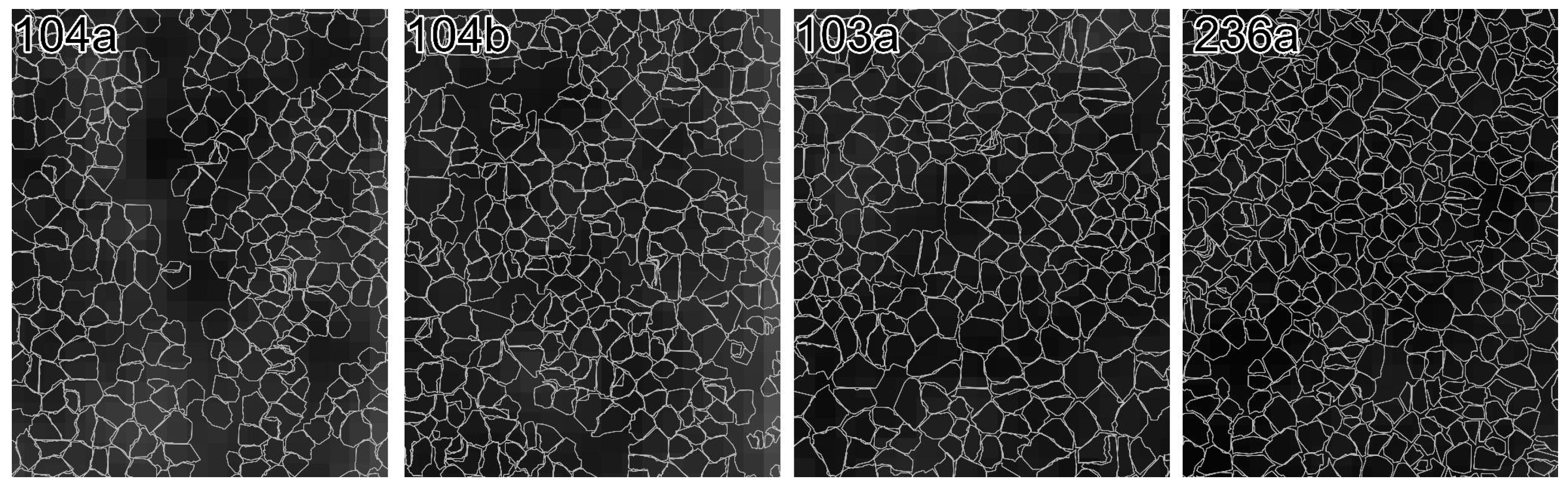
1. Introduction
- Establishing a clear relationship between observed LAI values and A. posticalis defoliation activity;
- Assessing the quality of empirical methods of LAI estimation via RS imagery.
2. Materials and Methods
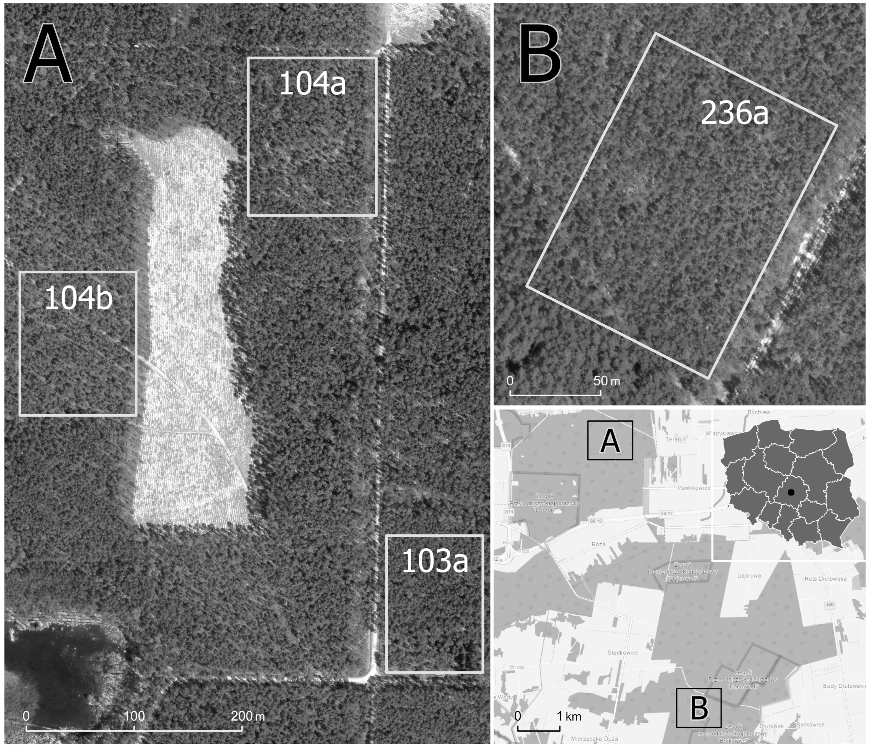
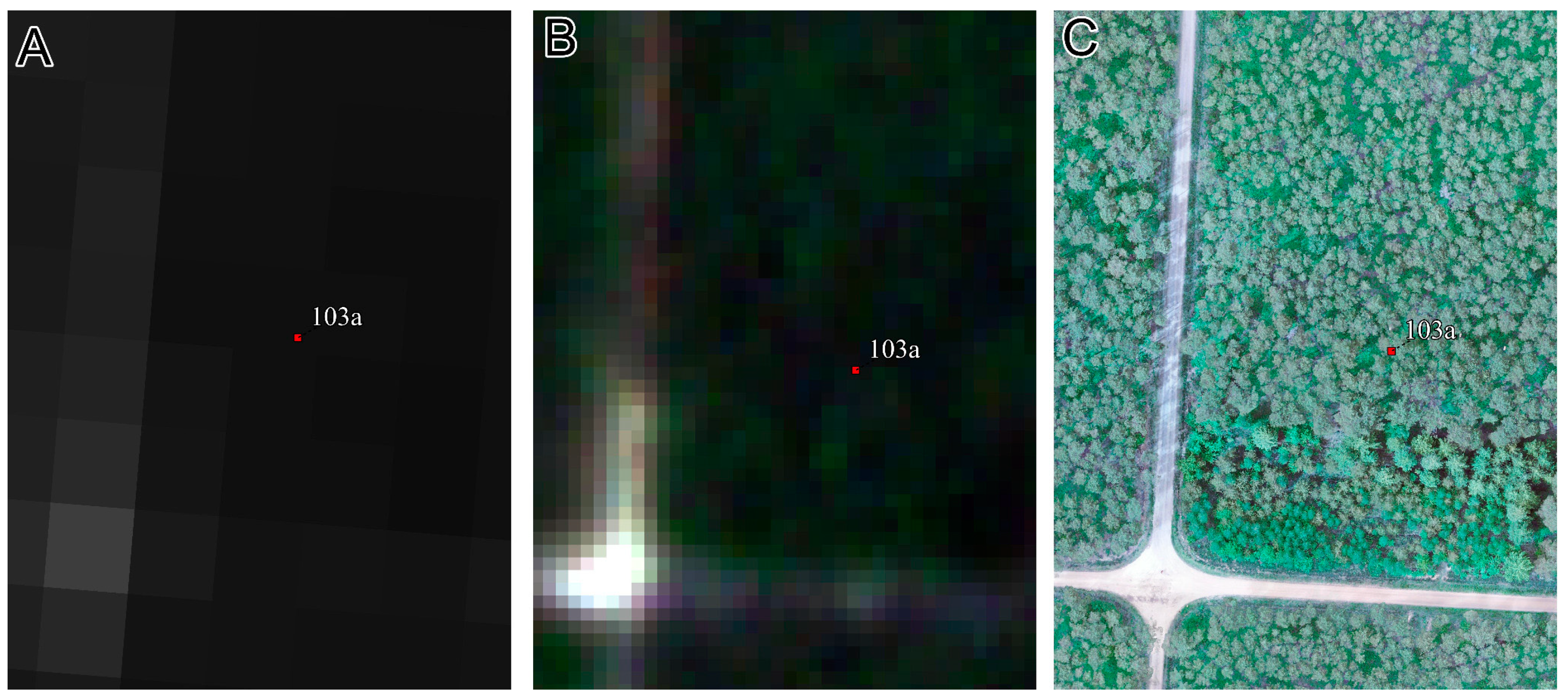
2.1. Area of Interest
2.2. Ground Observed Data
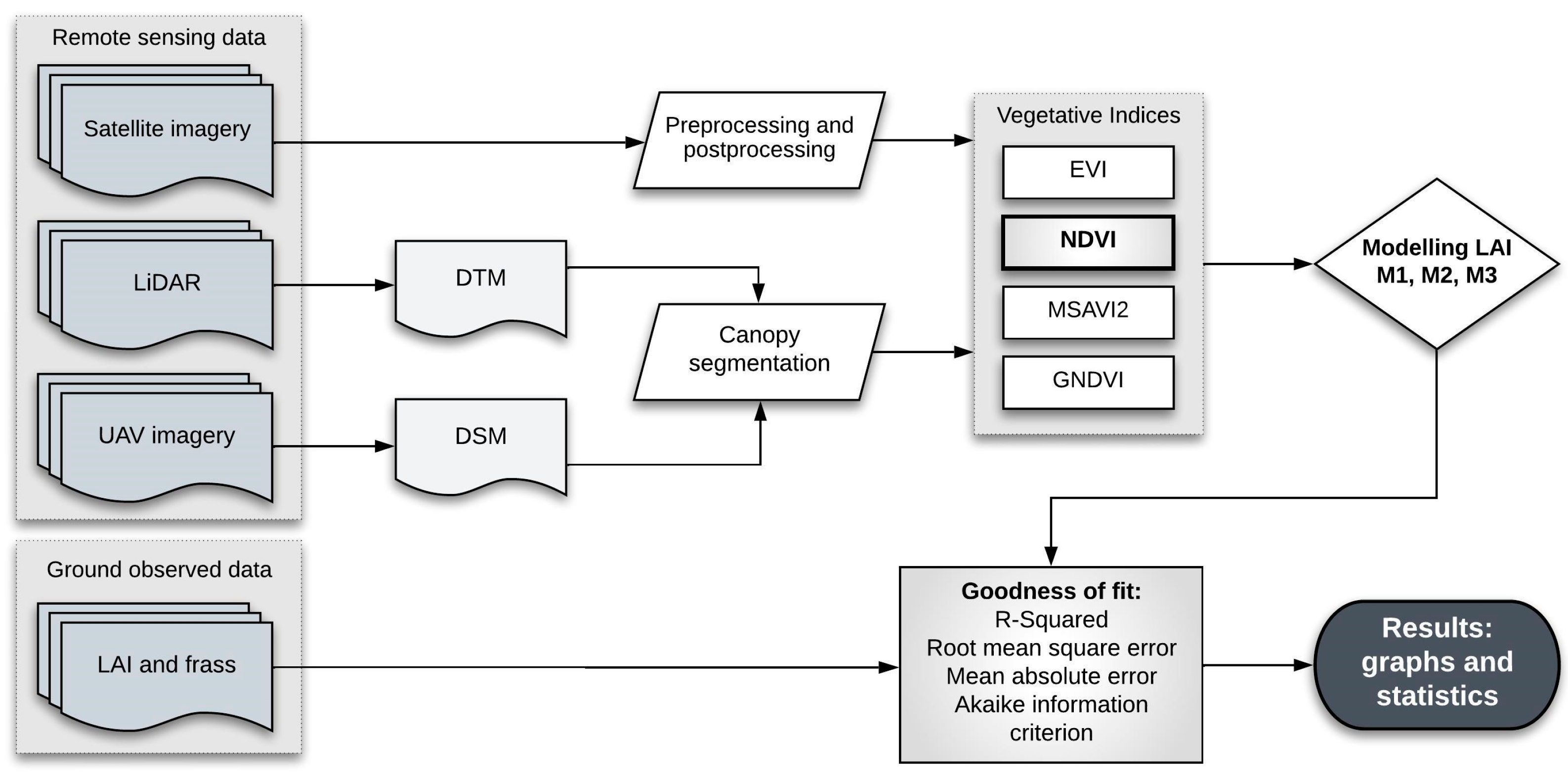
2.3. Remote Sensing Data
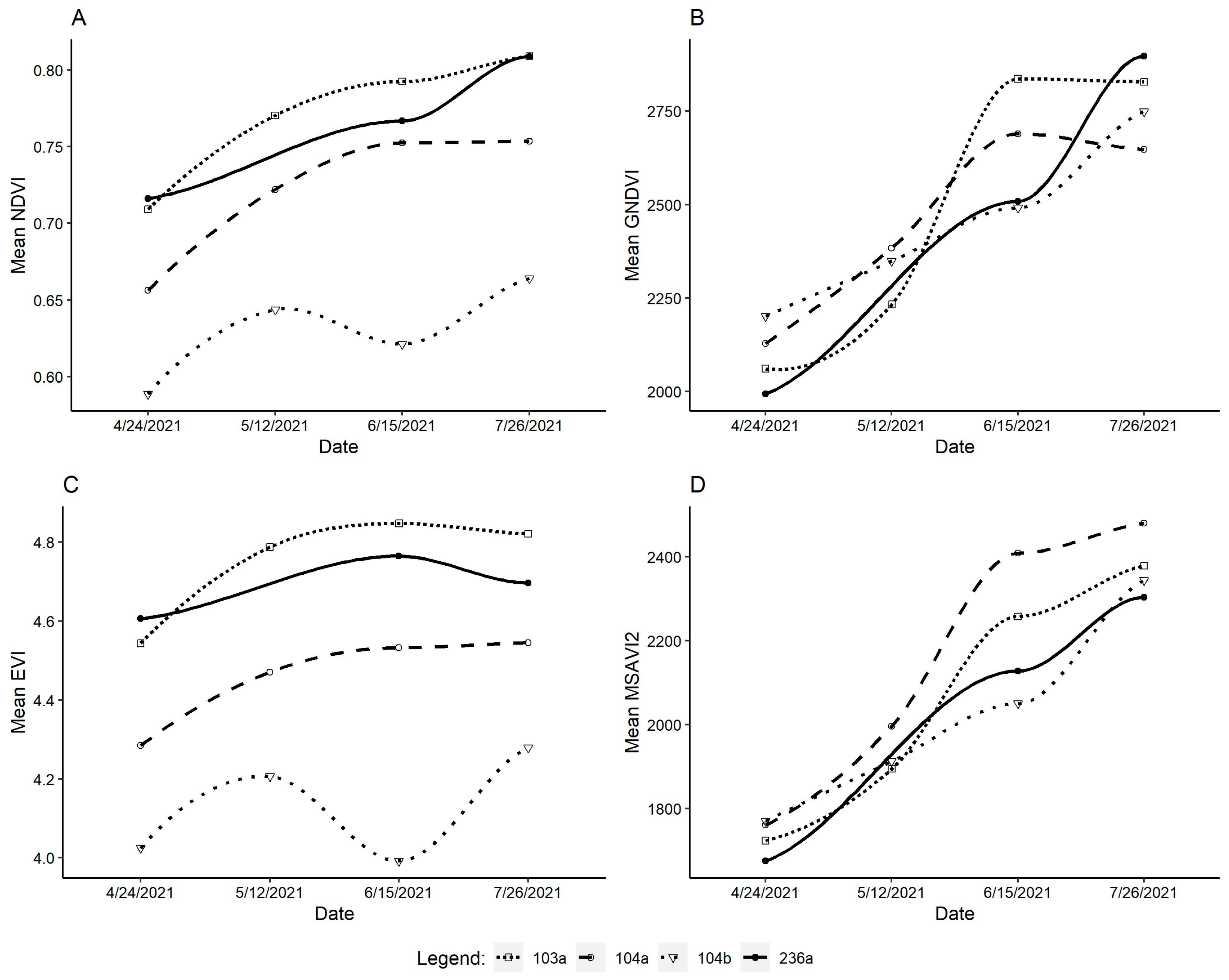
2.4. Vegetative Indices Selection
2.5. Canopy Segmentation
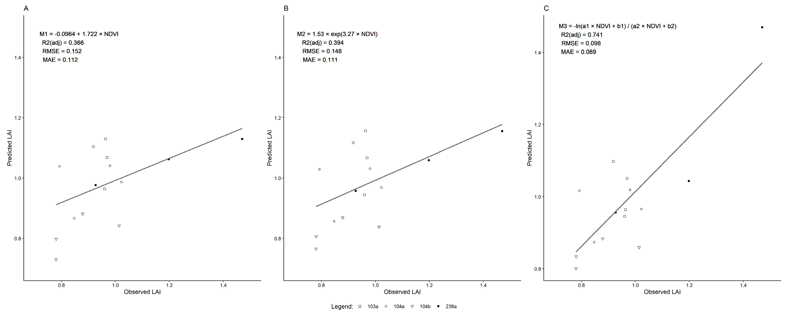
2.6. Modeling LAI
3. Results
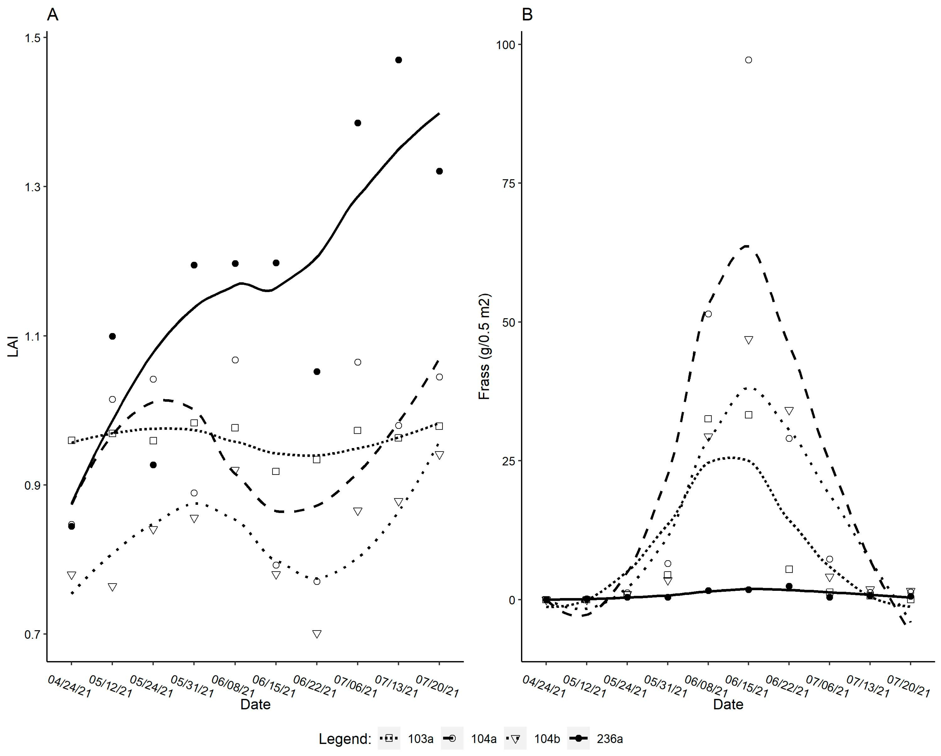
3.1. Ground Data
3.2. Vegetative Indices Results
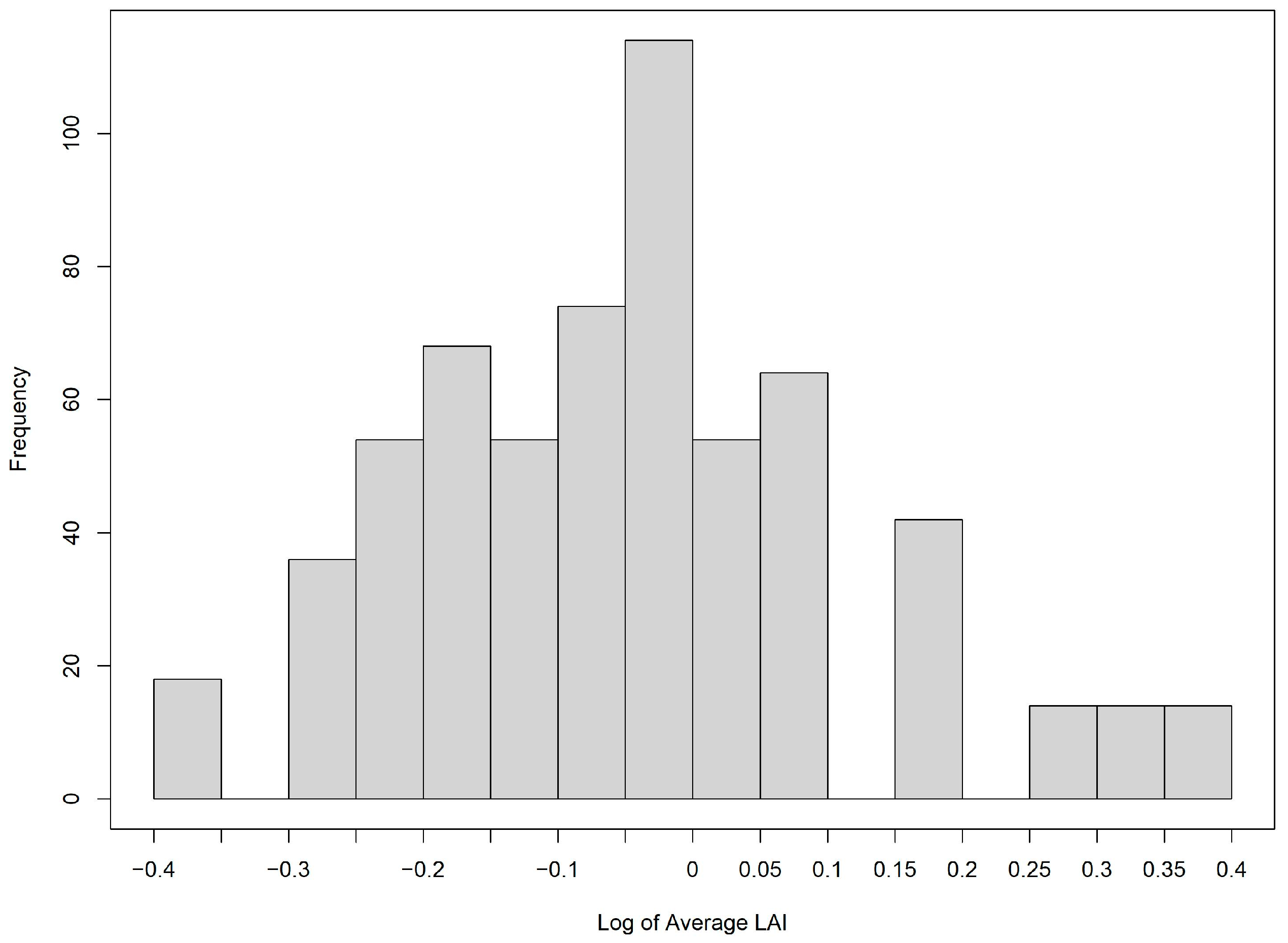
3.3. LAI Modeling
4. Discussion
4.1. The Relationship Between Acantholyda posticalis and Ground Observation Data
4.2. Influence of Ground Cover on Canopy Analysis in Remote Sensing
4.3. Study Limitations
4.4. Model Construction and Fitting
4.5. Impacts of Resolution
4.6. Remote Sensing Difficulties
4.7. LAI Modeling Confidence
4.8. Adaptation for Forest Management
- High-resolution multispectral imagery ≤ 0.5 m along with LiDAR point cloud data (though not presented in this study, a modified workflow that only uses LiDAR sensors could also be utilized);
- Employment of vegetative indices as a means of augmenting imagery to display underlaying biological responses;
- Development of a canopy segmentation that is capable of defining and labeling all unique individual crowns;
- Implementation of a model that accurately predicts LAI from sampled VI values that can later be used as the basis for constructing disturbance mapping.
4.9. Future Studies
5. Conclusions
- LAI, as a qualitative measure, is significantly correlated with A. posticalis defoliation disturbance in the context of a managed P. sylvestris stand;
- LAI can be modeled from vegetative index values in a way that is significantly similar to ground-observed LAI values;
- High spatial resolution (≤50 cm) is absolutely required to investigate insect defoliation disturbance using remote sensing methods in the context of small time scales and forestry application.
Author Contributions
Funding
Data Availability Statement
Conflicts of Interest
References
- Seidl, R.; Schelhaas, M.-J.; Lexer, M.J. Unraveling the Drivers of Intensifying Forest Disturbance Regimes in Europe. Glob. Change Biol. 2011, 17, 2842–2852. [Google Scholar] [CrossRef]
- Kautz, M.; Meddens, A.J.H.; Hall, R.J.; Arneth, A. Biotic Disturbances in Northern Hemisphere Forests—A Synthesis of Recent Data, Uncertainties and Implications for Forest Monitoring and Modelling. Glob. Ecol. Biogeogr. 2017, 26, 533–552. [Google Scholar] [CrossRef]
- Voolma, K.; Pilt, E.; Õunap, H. The First Reported Outbreak of the Great Web-Spinning Pine-Sawfly, Acantholyda posticalis (Mats.) (Hymenoptera, Pamphiliidae), in Estonia. For. Stud. 2009, 50, 115–122. [Google Scholar] [CrossRef]
- Viitasaari, M. Sawflies (Hymenoptera, Symphyta) I. Zoosystematics Evol. 2004, 80, 135. [Google Scholar] [CrossRef]
- Głowacka, B.; Skrzecz, I.; Bystrowski, C. Reducing the abundance of great pine web−spinning pine sawfly Acantholyda posticalis Mats. in pine stands. Sylwan 2014, 158, 323–330. [Google Scholar]
- Sławski, M.; Mokrzycki, T.; Perliński, S.; Rutkiewicz, A.; Sławska, M. Distribution of wintering pre-imaginal stages of the great web-spinning pine sawfly Acantholyda posticalis Mats. in Scots pine stands being the outbreak centres. Sylwan 2019, 163, 556–563. [Google Scholar] [CrossRef]
- Voolma, K.; Hiiesaar, K.; Williams, I.H.; Ploomi, A.; Jõgar, K. Cold Hardiness in the Pre-imaginal Stages of the Great Web-spinning Pine-sawfly Acantholyda posticalis. Agric. For. Entomol. 2016, 18, 432–436. [Google Scholar] [CrossRef]
- Raffa, K.F.; Aukema, B.H.; Bentz, B.J.; Carroll, A.L.; Hicke, J.A.; Turner, M.G.; Romme, W.H. Cross-Scale Drivers of Natural Disturbances Prone to Anthropogenic Amplification: The Dynamics of Bark Beetle Eruptions. BioScience 2008, 58, 501–517. [Google Scholar] [CrossRef]
- Senf, C.; Seidl, R.; Hostert, P. Remote Sensing of Forest Insect Disturbances: Current State and Future Directions. Int. J. Appl. Earth Obs. Geoinf. 2017, 60, 49–60. [Google Scholar] [CrossRef]
- Mngadi, M.; Germishuizen, I.; Mutanga, O.; Naicker, R.; Maes, W.H.; Odebiri, O.; Schroder, M. A Systematic Review of the Application of Remote Sensing Technologies in Mapping Forest Insect Pests and Diseases at a Tree-Level. Remote Sens. Appl. Soc. Environ. 2024, 36, 101341. [Google Scholar] [CrossRef]
- Frost, C.J.; Hunter, M.D. Insect Canopy Herbivory and Frass Deposition Affect Soil Nutrient Dynamics and Export in Oak Mesocosms. Ecology 2004, 85, 3335–3347. [Google Scholar] [CrossRef]
- Zheng, G.; Moskal, L.M. Retrieving Leaf Area Index (LAI) Using Remote Sensing: Theories, Methods and Sensors. Sensors 2009, 9, 2719–2745. [Google Scholar] [CrossRef] [PubMed]
- De Bei, R.; Fuentes, S.; Gilliham, M.; Tyerman, S.; Edwards, E.; Bianchini, N.; Smith, J.; Collins, C. VitiCanopy: A Free Computer App to Estimate Canopy Vigor and Porosity for Grapevine. Sensors 2016, 16, 585. [Google Scholar] [CrossRef] [PubMed]
- Marques Ramos, A.P.; Prado Osco, L.; Elis Garcia Furuya, D.; Nunes Gonçalves, W.; Cordeiro Santana, D.; Pereira Ribeiro Teodoro, L.; Antonio Da Silva Junior, C.; Fernando Capristo-Silva, G.; Li, J.; Henrique Rojo Baio, F.; et al. A Random Forest Ranking Approach to Predict Yield in Maize with Uav-Based Vegetation Spectral Indices. Comput. Electron. Agric. 2020, 178, 105791. [Google Scholar] [CrossRef]
- Morales-Gallegos, L.M.; Martínez-Trinidad, T.; Hernández-de La Rosa, P.; Gómez-Guerrero, A.; Alvarado-Rosales, D.; Saavedra-Romero, L.D.L. Tree Health Condition in Urban Green Areas Assessed through Crown Indicators and Vegetation Indices. Forests 2023, 14, 1673. [Google Scholar] [CrossRef]
- Congedo, L. Semi-Automatic Classification Plugin Documentation. Release 5.0.0.1 2016, 4, 29. [Google Scholar]
- Daniel, W.W.; Cross, C.L. Biostatistics: A Foundation for Analysis in the Health Sciences, 11th ed.; Wiley: Hoboken, NJ, USA, 2018; ISBN 978-1-119-49657-1. [Google Scholar]
- Akoglu, H. User’s Guide to Correlation Coefficients. Turk. J. Emerg. Med. 2018, 18, 91–93. [Google Scholar] [CrossRef]
- Oruba, A.; Ryczywolski, M.; Wajda, S.; Bosy, J.; Graszka, W.; Leończyk, M.; Somla, J. The Implementation of the Precise Satellite Positioning System ASG-EUPOS. In Proceedings of the ENC-GNSS 2008 Conference Proceedings, EUGIN, Toulouse, France, 23–25 April 2008. [Google Scholar]
- Mamouei, M.; Budidha, K.; Baishya, N.; Qassem, M.; Kyriacou, P.A. An Empirical Investigation of Deviations from the Beer–Lambert Law in Optical Estimation of Lactate. Sci. Rep. 2021, 11, 13734. [Google Scholar] [CrossRef]
- Saito, K.; Ogawa, S.; Aihara, M.; Otowa, K. Estimates of LAI for Forest Management in Okutama. In Proceedings of the 22nd ACRS Conference on Remote Sensing, Singapore, 5–9 November 2001; Rissho University: Kumagaya, Japan, 2001; Volume 1, pp. 600–605. [Google Scholar]
- Fan, L.; Gao, Y.; Brück, H.; Bernhofer, C. Investigating the Relationship between NDVI and LAI in Semi-Arid Grassland in Inner Mongolia Using in-Situ Measurements. Theor. Appl. Clim. 2009, 95, 151–156. [Google Scholar] [CrossRef]
- Tan, C.-W.; Zhang, P.-P.; Zhou, X.-X.; Wang, Z.-X.; Xu, Z.-Q.; Mao, W.; Li, W.-X.; Huo, Z.-Y.; Guo, W.-S.; Yun, F. Quantitative Monitoring of Leaf Area Index in Wheat of Different Plant Types by Integrating NDVI and Beer-Lambert Law. Sci. Rep. 2020, 10, 929. [Google Scholar] [CrossRef]
- Olsson, P.-O.; Kantola, T.; Lyytikäinen-Saarenmaa, P.; Jönsson, A.; Eklundh, L. Development of a Method for Monitoring of Insect Induced Forest Defoliation—Limitation of MODIS Data in Fennoscandian Forest Landscapes. Silva Fenn. 2016, 50, 1495. [Google Scholar] [CrossRef]
- Zhao, Y.; Chen, X.; Smallman, T.L.; Flack-Prain, S.; Milodowski, D.T.; Williams, M. Characterizing the Error and Bias of Remotely Sensed LAI Products: An Example for Tropical and Subtropical Evergreen Forests in South China. Remote Sens. 2020, 12, 3122. [Google Scholar] [CrossRef]
- Rosso, P.; Nendel, C.; Gilardi, N.; Udroiu, C.; Chlebowski, F. Processing of Remote Sensing Information to Retrieve Leaf Area Index in Barley: A Comparison of Methods. Precis. Agric. 2022, 23, 1449–1472. [Google Scholar] [CrossRef]
- Debeurs, K.; Townsend, P. Estimating the Effect of Gypsy Moth Defoliation Using MODIS. Remote Sens. Environ. 2008, 112, 3983–3990. [Google Scholar] [CrossRef]
- Eriksson, H.M.; Eklundh, L.; Kuusk, A.; Nilson, T. Impact of Understory Vegetation on Forest Canopy Reflectance and Remotely Sensed LAI Estimates. Remote Sens. Environ. 2006, 103, 408–418. [Google Scholar] [CrossRef]
- Duarte, A.; Borralho, N.; Cabral, P.; Caetano, M. Recent Advances in Forest Insect Pests and Diseases Monitoring Using UAV-Based Data: A Systematic Review. Forests 2022, 13, 911. [Google Scholar] [CrossRef]
- De Wit, C.T. Photosynthesis of Leaf Canopies; PUDOC: Wageningen, Germany, 1965; pp. 1–57. [Google Scholar]
- Jia, K.; Liang, S.; Zhang, L.; Wei, X.; Yao, Y.; Xie, X. Forest Cover Classification Using Landsat ETM+ Data and Time Series MODIS NDVI Data. Int. J. Appl. Earth Obs. Geoinf. 2014, 33, 32–38. [Google Scholar] [CrossRef]
- Li, Y.; Li, M.; Li, C.; Liu, Z. Forest Aboveground Biomass Estimation Using Landsat 8 and Sentinel-1A Data with Machine Learning Algorithms. Sci. Rep. 2020, 10, 9952. [Google Scholar] [CrossRef]
- Lovynska, V.; Sytnyk, S.; Stankevich, S.; Holoborodko, K.; Tkalich, Y.; Nikovska, I.; Bandura, L.; Buchavuy, Y. Aboveground Biomass Estimation in Conifer and Deciduous Forests with the Use of a Combined Approach. Biosys. Divers. 2024, 32, 210–216. [Google Scholar] [CrossRef]
- Maselli, F. Monitoring Forest Conditions in a Protected Mediterranean Coastal Area by the Analysis of Multiyear NDVI Data. Remote Sens. Environ. 2004, 89, 423–433. [Google Scholar] [CrossRef]
- Miraki, M.; Sohrabi, H.; Fatehi, P.; Kneubuehler, M. Detection of Mistletoe Infected Trees Using UAV High Spatial Resolution Images. J. Plant Dis. Prot. 2021, 128, 1679–1689. [Google Scholar] [CrossRef]
- Motohka, T.; Nasahara, K.N.; Oguma, H.; Tsuchida, S. Applicability of Green-Red Vegetation Index for Remote Sensing of Vegetation Phenology. Remote Sens. 2010, 2, 2369–2387. [Google Scholar] [CrossRef]
- Santoro, M.; Cartus, O.; Carvalhais, N.; Rozendaal, D.M.A.; Avitabile, V.; Araza, A.; De Bruin, S.; Herold, M.; Quegan, S.; Rodríguez-Veiga, P.; et al. The Global Forest Above-Ground Biomass Pool for 2010 Estimated from High-Resolution Satellite Observations. Earth Syst. Sci. Data 2021, 13, 3927–3950. [Google Scholar] [CrossRef]
- Schrader-Patton, C.; Grulke, N.; Bienz, C. Assessment of Ponderosa Pine Vigor Using Four-Band Aerial Imagery in South Central Oregon: Crown Objects to Landscapes. Forests 2021, 12, 612. [Google Scholar] [CrossRef]
- Usta, A.; Yilmaz, M. Prediction of Pine Mistletoe Infection Using Remote Sensing Imaging: A Comparison of the Artificial Neural Network Model and Logistic Regression Model. For. Pathol. 2023, 53, e12783. [Google Scholar] [CrossRef]
- Lacasa, J.; Hefley, T.J.; Otegui, M.E.; Ciampitti, I.A. A Practical Guide to Estimating the Light Extinction Coefficient with Nonlinear Models—A Case Study on Maize. Plant Methods 2021, 17, 60. [Google Scholar] [CrossRef]


| Data | Observed LAI | Frass (g/0.5 m2) | ||||||
|---|---|---|---|---|---|---|---|---|
| Infested Plots | Control Plot | Infested Plots | Control Plot | |||||
| 103a | 104a | 104b | 236a | 103a | 104a | 104b | 236a | |
| 24.04.21 | 0.960 | 0.847 | 0.780 | 0.845 | n/a | n/a | n/a | n/a |
| 12.05.21 | 0.969 | 1.015 | 0.764 | 1.099 | 0 | 0.135 | 0 | 0.148 |
| 24.05.21 | 0.960 | 1.042 | 0.841 | 0.927 | 0.826 | 1.275 | 0.998 | 0.442 |
| 31.05.21 | 0.983 | 0.889 | 0.856 | 1.195 | 4.453 | 6.542 | 3.514 | 0.445 |
| 08.06.21 | 0.977 | 1.068 | 0.920 | 1.197 | 32.58 | 51.47 | 29.38 | 1.652 |
| 15.06.21 | 0.918 | 0.793 | 0.780 | 1.198 | 33.27 | 97.19 | 46.94 | 1.833 |
| 22.06.21 | 0.934 | 0.771 | 0.701 | 1.052 | 5.478 | 29.057 | 34.172 | 2.447 |
| 06.07.21 | 0.973 | 1.065 | 0.866 | 1.385 | 1.362 | 7.297 | 4.139 | 0.471 |
| 13.07.21 | 0.963 | 0.980 | 0.879 | 1.470 | 0.732 | 1.317 | 1.873 | 0.735 |
| 20.07.21 | 0.979 | 1.045 | 0.941 | 1.321 | n/a | 1.35 | 1.604 | 0.606 |
| Variable | Plot | N | Mean | St.Dev | Min | Q1 | Q3 | Max |
|---|---|---|---|---|---|---|---|---|
| Observed Frass (g/0.5 m2) | All Plots | 35 | 12.4 | 21.6 | 0 | 0.7 | 7.3 | 97.2 |
| Observed LAI | 104a | 10 | 0.951 | 0.11 | 0.771 | 0.847 | 1.045 | 1.068 |
| 104b | 10 | 0.833 | 0.071 | 0.701 | 0.78 | 0.879 | 0.941 | |
| 103a | 10 | 0.962 | 0.02 | 0.918 | 0.96 | 0.977 | 0.983 | |
| 236a | 10 | 1.169 | 0.186 | 0.845 | 1.052 | 1.321 | 1.47 | |
| All Plots | 40 | 0.968 | 0.165 | 0.701 | 0.847 | 1.045 | 1.47 | |
| M3 Modeled LAI | 104a | 390 | 1.043 | 0.155 | 0.724 | 0.916 | 1.159 | 1.482 |
| 104b | 264 | 0.843 | 0.092 | 0.607 | 0.81 | 0.909 | 1.044 | |
| 103a | 228 | 1.276 | 0.162 | 0.914 | 1.184 | 1.404 | 1.736 | |
| 236a | 255 | 1.248 | 0.176 | 0.907 | 1.133 | 1.396 | 1.688 | |
| All Plots | 1137 | 1.005 | 0.169 | 0.8 | 0.884 | 1.044 | 1.47 | |
| Pixel DNV | NDVI | 1137 | 0.726 | 0.065 | 0.589 | 0.664 | 0.77 | 0.809 |
| GNDVI | 1137 | 2521.71 | 269.021 | 1993.06 | 2348.59 | 2749.32 | 2896.86 | |
| EVI | 1137 | 4.505 | 0.261 | 3.992 | 4.284 | 4.765 | 4.848 | |
| MAVI2 | 1137 | 31.763 | 55.06 | 74.032 | 12.382 | 44.5 | 80.128 |
| Regressions | Estimate | SE | t-Value | p-Value |
|---|---|---|---|---|
| LAI~Frass (g/0.5 m2) | −0.052 | 0.013 | −3.873 | 0.000303 *** |
| M1~Observed LAI | 0.730 | 0.029 | 25.62 | <2 × 10¹⁶ *** |
| M2~Observed LAI | 0.791 | 0.029 | 27.19 | <2 × 10¹⁶ *** |
| Predicted LAI (236a)~Observed LAI | 1.213 | 0.008 | 161.36 | <2 × 10¹⁶ *** |
| Predicted LAI (104b)~Observed LAI | 1.260 | 0.098 | 12.93 | 0.0128 * |
| Correlation | rho |
|---|---|
| NDVI~Observed LAI | 0.612 ** |
| GNDVI~Observed LAI | 0.374 ** |
| EVI~Observed LAI | 0.536 ** |
| MSAVI2~Observed LAI | 0.205 ** |
| Parameter | Estimate | SE | t-Value | p-Value |
|---|---|---|---|---|
| a1 | −4.247 | 0.229 | −18.54 | <2 × 10¹⁶ *** |
| a2 | 3.747 | 0.177 | 21.19 | <2 × 10¹⁶ *** |
| b1 | 4.435 | 0.185 | 23.93 | <2 × 10¹⁶ *** |
| b2 | −3.031 | 0.143 | −21.19 | <2 × 10¹⁶ *** |
| Models | df | AIC | R2 | RMSE | MAE |
|---|---|---|---|---|---|
| M1 | 1135 | −1045.528 | 0.3658 | 0.152 | 0.112 |
| M2 | 1135 | −1097.196 | 0.39397 | 0.148 | 0.111 |
| M3 | 1133 | −1942.804 | 0.74 | 0.098 | 0.069 |
Disclaimer/Publisher’s Note: The statements, opinions and data contained in all publications are solely those of the individual author(s) and contributor(s) and not of MDPI and/or the editor(s). MDPI and/or the editor(s) disclaim responsibility for any injury to people or property resulting from any ideas, methods, instructions or products referred to in the content. |
© 2025 by the authors. Licensee MDPI, Basel, Switzerland. This article is an open access article distributed under the terms and conditions of the Creative Commons Attribution (CC BY) license (https://creativecommons.org/licenses/by/4.0/).
Share and Cite
Seymour, J.; Brach, M.; Sławski, M. A Small-Scale Investigation into the Viability of Detecting Canopy Damage Caused by Acantholyda posticalis Disturbance Using High-Resolution Satellite Imagery in a Managed Pinus sylvestris Stand in Central Poland. Forests 2025, 16, 472. https://doi.org/10.3390/f16030472
Seymour J, Brach M, Sławski M. A Small-Scale Investigation into the Viability of Detecting Canopy Damage Caused by Acantholyda posticalis Disturbance Using High-Resolution Satellite Imagery in a Managed Pinus sylvestris Stand in Central Poland. Forests. 2025; 16(3):472. https://doi.org/10.3390/f16030472
Chicago/Turabian StyleSeymour, Jackson, Michał Brach, and Marek Sławski. 2025. "A Small-Scale Investigation into the Viability of Detecting Canopy Damage Caused by Acantholyda posticalis Disturbance Using High-Resolution Satellite Imagery in a Managed Pinus sylvestris Stand in Central Poland" Forests 16, no. 3: 472. https://doi.org/10.3390/f16030472
APA StyleSeymour, J., Brach, M., & Sławski, M. (2025). A Small-Scale Investigation into the Viability of Detecting Canopy Damage Caused by Acantholyda posticalis Disturbance Using High-Resolution Satellite Imagery in a Managed Pinus sylvestris Stand in Central Poland. Forests, 16(3), 472. https://doi.org/10.3390/f16030472