Article

Biomass Allometries for Urban Trees: A Case Study in Athens, Greece

by
Magdalini Dapsopoulou
1,2 and
Dimitris Zianis
1,*
1
Department of Forestry and Natural Environment Management, School of Plant Sciences, Agricultural University of Athens, 36100 Karpenisi, Greece
2
Department of Greenery & Urban Fauna, Municipality of Athens, 11527 Athens, Greece
*
Author to whom correspondence should be addressed.
Forests 2025, 16(3), 466; https://doi.org/10.3390/f16030466
Submission received: 13 February 2025 / Revised: 27 February 2025 / Accepted: 28 February 2025 / Published: 6 March 2025
(This article belongs to the Special Issue Urban Green Infrastructure and Urban Landscape Ecology)

Abstract

:
Urban street trees often exhibit distinct architectural characteristics compared to their counterparts in natural forests. Allometric equations for the stem (MS), branches (MB), and total dry aboveground biomass of urban trees (MT) were developed, based on 52 destructively sampled specimens, belonging to 10 different species, growing in the Municipality of Athens, Greece. Linear, log-linear, and nonlinear regression analyses were applied, and fit statistics were used to select the most appropriate model. The results indicated that diameter at breast height (D1.3) and tree height (H) are needed for accurately predicting MS, while MB may be estimated based on D1.3. To circumvent the caveat of the additivity property for estimating the biomass of different tree component, nonlinear seemingly unrelated regression (NSUR) was implemented. The 95% prediction intervals for MS, MB, and MT efficiently captured the variability of the sampled trees. Finally, the predictions were compared with estimates from i-Tree, the most widely used model suite for urban and rural forestry analysis, and a mean deviation of 134% (ranging from 3% to 520%) was reported. Therefore, in the absence of urban-specific allometries, the obtained empirical models are proposed for estimating biomass in street trees, particularly in cities with Mediterranean-like climatic influences.

1. Introduction

The adverse effects of urbanization on the environment are mitigated through the benefits provided by the functional and structural properties of green spaces. Green spaces play a multifaceted role, such as improving air quality, adjusting temperatures, decreasing soil water depletion, etc. Tree species constitute a critical component for urban green spaces, since the organic matter sustained by individuals belonging to different taxa largely contributes to the multifunctionality of these ecosystems. The reported absence of statistically robust estimations of volume and biomass production for urban trees [1,2] is a significant constraint towards an integrated analysis of urban ecosystems. To circumvent quantitative problems related to the sustainable planning of urban green spaces, managers use empirical equations developed for trees growing in forested ecosystems [3,4,5].
For instance, even though i-Tree [6,7] is one of the most widely used urban tree platforms, cited in 8461 research articles across 21 countries [8], the built-in empirical equations for estimating aboveground tree biomass (M) were derived mainly from trees growing in forested stands. On contrast, street trees experience human-induced, biotic, and abiotic effects, which are totally different in intense and extremity than the ones affecting their counterparts growing in forested conditions. For example, Pinkard & Beadle [9] reported that pruning urban trees reduced both branch diameter and length in the upper crowns of Eucalyptus nitens, whereas it did not affect branch extension length and branch growth rate in Pinus radiate trees [10].
Both in forest stands and in open-grown trees, height growth is prioritized in the early stages of development, followed by increased investment in stem (cambial) growth as the tree matures. Moreover, urban trees may inherently prioritize resource allocation towards cambial growth [11,12], whereas forest trees typically allocate resources to height growth, initiating branching near the apical meristem. This differentiation in growth habits may affect the production of organic matter, and in turn introduce systematic errors in predicting M for urban specimens, in case forest-based allometries are to be used.
McHale et al. [13] noted that in order to derive M for open-grown trees, predictions obtained for forest trees are usually reduced by a factor of 0.8 due to the lack of empirical equations for estimating dry biomass for urban trees. They compared M predictions from allometries built for urban trees in Colorado (USA) to those derived from trees growing in forests. While some published equations for forest trees provided similar biomass estimates to urban-based predictions, the variability for individual trees reached up to 300%. This variability was reduced at larger scales, dropping to 60% for a community of street trees comprising 11 species and 10,551 trees [13]. Although errors in biomass estimates were reduced when including a diverse range of species, a 60% variability is still significant, suggesting that researchers should be very cautious when selecting allometric equations and interpreting their results. Similarly, findings by Yoon et al. [14] indicated that equations developed for forest trees tended to overestimate M in comparison to equations for urban trees by 68 to 427%. As Yang et al. [15] highlighted in their review of methods for quantifying and estimating urban trees biomass, the variability in M predictions underscores the need for more tailored approaches in urban settings.
Pillsbury and Reiner [16] developed empirical volume equations for urban trees growing in California and highlighted the shortage of allometries for green spaces. The derived volumetric predictions were used by urban forest managers to estimate wood residue, and are now used under the context of greenhouse gas offsets [6].
There are many empirical equations relating the biomass (M) of forest trees to their linear dimensions (e.g., stem diameter at 1.3 m above the ground; D1.3). These equations often follow the simple power mathematical function which is called allometry in biological modelling [17]:
M = aD1.3b
The theoretical framework and the practical utility of this model have been extensively reported in the literature ([18,19,20,21,22,23,24,25,26,27], to name but a few). Statistically, this equation can be classified into two types of regression models: the “intrinsically linear”, which assumes a multiplicative error structure and requires log-transformation, and the “intrinsically nonlinear”, which incorporates an additive random error in the raw data [28].
Another statistical feature pertaining to M estimation is the additivity property of tree components [29,30,31]. In other words, the sum of the predictions for different M components (stem, branches, foliage, roots, etc.) should be equal to the prediction for total tree biomass. This issue mainly originates from the destructive sampling of biomass components; M measurements performed in different tree components are added up to provide the organic matter for the whole tree. To address this property, the simultaneous estimation approach has long been proposed [32,33]. Zellner [34] proposed the seemingly unrelated nonlinear regressions (NSUR) technique, utilizing the simultaneous estimation approach which was further exemplified by Parresol [29] and Parresol [30]. Specific methods to ensure the additivity of regression functions are presented in [35]. The heteroscedasticity problem (non-constant variance of M predictions across the independent variable range) is another issue in allometric studies. As Parresol [36] discusses, the error variance is usually related to the explanatory variable(s) of the model and can be incorporated in the fitting process algorithm.
Although numerous studies have developed empirical equations to describe size–shape relationships for urban trees, a significant issue with most of these analyses is that they lack direct measurement of urban tree volume and biomass [1,2]. Most studies quantifying the benefits and costs associated with urban trees and their management use allometric equations originally developed for trees in traditional forests [3,4,5]. Despite the extensive development of these equations worldwide, biomass allometries for urban trees are largely missing from the literature. Thus, the first objective of this study is to develop empirical allometric equations to robustly and efficiently predict M for trees located in the metropolitan area of Athens, Greece. The second objective is to demonstrate the appropriateness of i-Tree, a software suite designed for urban and rural forestry analysis, in predicting the aboveground carbon content of Mediterranean urban trees.

2. Materials and Methods

2.1. Study Area

Raw biomass datasets were collected from the Municipality of Athens, the most populous municipality and the capital of Greece, with 643,452 permanent residents. The metropolitan area of Athens has approximately 2.7 million inhabitants [37].

2.1.1. Morphology and Topology

The city of Athens is located within the basin of Attica and is the center of Metropolitan Athens. It is located at an altitude of 130 m above sea level, at latitude 38° and longitude 24°, and occupies an area of 39 km2. The basin is surrounded by four mountain masses: Parnitha to the north, Aigaleo to the west, Hymettos to the east, and Penteli to the northeast, while to the south it is washed by the Saronic Gulf. This particular geomorphology favors the formation of temperature inversions. The temperature inversion creates a stabilized state in the atmosphere and blocks the movement of gas masses. As a result, gaseous pollutants are trapped in the atmosphere and incidents of air pollution are created (soot 8), according to the Municipality of Athens [38].

2.1.2. Climate

The climate of Athens is characterized as subtropical, Mediterranean, with prolonged hot and dry summers, mild winters, and moderate rainfall. The average temperature is 17.7 °C, based on the local weather station of the Thisio area. In the center of the municipality, quite elevated temperatures in the summer season have been recorded, while during the December–March period the temperature can drop below 0 °C. The highest temperature for all of Europe was recorded in Athens on 10 July 1977, reaching 48 °C. The average rainfall is relatively low (378 mm per year), as well as the wind speed (around 2 m/s annual average wind intensity) [39,40].
In addition, due to the intense sunshine, during the summer months Athens has frequent occurrences of photochemical pollution episodes. Athens is also strongly affected by the urban heat island phenomenon. This phenomenon refers to the appearance of higher temperatures in areas of the city where there is dense construction and a lack of greenery and air movement compared to neighboring greener areas. During days with high temperatures, the western parts of the Municipality of Athens show a 3–4 °C temperature difference (on average) compared to other parts of the city [38].

2.1.3. Tree-Level Data

In total, fifty-two (52) trees were randomly selected across the Municipality of Athens and destructively sampled during the growth period of 2023. The sampled trees exhibited diverse structural conditions, with some displaying evidence of recurrent pruning, topping, and other anthropogenic influences such as soil compaction and vandalism.
Total tree height (H, in m) and stem height from the base of the tree to the starting point of the tree crown (Hs) were measured for each sample before cutting, using Nikon’s Laser Forestry Pro II (Distance-Measuring Monocular). The diameter at 0.3 m above ground (D0.3, in cm), the diameter at breast height (D1.3, in cm), and the diameter at the base of the crown (DC, in cm) were measured using diameter tape. Basal areas of the corresponding diameters were also calculated (i.e., B0.3, B1.3, and BC, in m2). The logs were weighed in the field and their fresh mass was measured using an electronic balance. Several discs (sub-samples) were removed from each log and their fresh weight was also determined in the field.
Branch sub-samples were selected from each tree as cutting progressed from the lower branches to the top, ensuring that they represented the size distribution of branches for the entire tree. The crown was divided into three equally spaced sections—upper, middle, and lower—and several sub-samples were taken from each part. The branches in each sub-sample were weighed and the fresh biomass was recorded.
To prevent moisture loss during transportation to the laboratory, all sub-samples (branch and stem discs) were placed in plastic bags, then dried in an oven at 104 °C until reaching a constant weight. The dry/fresh ratio of the sub-sampled data was used to estimate the dry biomass for each tree component in order to develop the empirical equations.
As a result, total aboveground dry biomass (MΤ, in kg) was calculated by the adding stem dry biomass (MS, in kg) to the dry biomass of branches (MB, in kg). In the biomass calculations, the sawdust at the time of cutting was not recorded.

2.2. Statistical Approaches

2.2.1. Solids of Revolution (Linear Approach)

Since size–shape allometries have not been thoroughly studied for urban trees, the modelling approach initiated within a ‘first’ principles framework. The linear dimensions of the sampled trees were used to derive predictions for MS, MB, and MT, assuming tree bole as a solid of revolution. The commonly applied approaches by Smallian and Newton were implemented to linearly regress biomass values against the basal areas, the tree height, and the length of the stem of the sampled specimens. The analyzed equations are reported in Appendix A.
Additionally, assuming that the shape of the tree may be approximated as a truncated cone or paraboloid, the following equation was used:
MT = s16D1.32H
The nlme R library, which includes the gls function, was used for this analysis [41].

2.2.2. Log-Linear Regression (Log Approach)

Assuming a multiplicative error structure in Equation (1), the values of the variables were log-transformed, and the following linear equation was obtained:
lnM = lna + blnD1.3 + lnε
which is commonly used to derive constant variance (homoscedasticity) across the range of the tree size, with lnε denoting the error of the predictions. Thus, the linear regression procedure can be applied in order to obtain estimates for lna and b. However, in back-transforming M predictions to normal scale, a correction factor is needed (CF), as reported in several studies [28,42,43,44].
M = a D 1.3 b   C F
According to Baskerville [42],
F = S E E 2 2 and CF = exp(F)
SEE stands for the standard error of the estimate of the linear regression and equals ( l n Y i l n Y i ^ ) 2 / ( n p ) ; n = number of observations, and p = number of parameters.
According to Yandle & Wiant [45], the systematic error or deviation of predictions or estimates from the true values, indicating inaccuracy in the model’s predictions, can be expressed and calculated using the formula:
Percent bias = ( ( e F 1 ) / e F ) 100
Wiant & Harner [46] considered it more informative to express the standard error of the estimated value Y ^ Corrected for a given X as a percentage of the estimated value Y ^ Corrected according to the formula:
Percent   standard   error = ( e F 1 ) 1 2 100

2.2.3. Generalized Nonlinear Least Squares (NLR Approach)

The conventional fitting approach for nonlinear regression (NLR) closely resembles the linear regression on the log-transformed data, with the distinction that it involves fitting a curve to the dataset instead of a straight line [35]. Similar to the linear case, the objective is to minimize the sum of the squares of both horizontal and vertical distances between the curve and the data points. To apply NLR regression, certain assumptions must be satisfied. In cases where no constant M variance is detected, appropriated weight variables can be used [29]. The intrinsically nonlinear functions analyzed are presented in the Appendix B. The nlme R library, which includes the gls function, was used for this analysis [41].

2.2.4. Nonlinear Seemingly Unrelated Regressions (NSUR)

According to Parresol [30], the additivity property of biomass equations is insured by setting constraints on the regression coefficients. The first step in NSUR is to apply the most appropriate empirical equation for each biomass component. In turn, restrictions to the parameters of the structural equations can be inserted so as the component equations to be simultaneously adjusted.
The system of the three contemporaneously correlated nonlinear biomass models was formulated as
MS = f1(X, β) + ε1
MB = f2(X, β) + ε2
MT = f3(X, β) + ε3
where X denotes the matrix of explanatory variables and β the parameters vector. Alternatively, setting
M = M S M B M T ,   f = f 1 f 2 f 3 and ε = ε 1 ε 2 ε 3 the following equation can be derived
M = f(X, β) + ε
Thus, the same explanatory variables and parameters are allowed to be common in some of the analyzed equations [30]. If weights are to be used, a matrix of weights in block-diagonal form [29] can also be incorporated into the analysis [30]. To build the structure in Equation (4), the most appropriate function for each component should be selected. To apply the NSUR algorithm in the sampled trees, the nlsur library in R was used for this analysis [47].

2.2.5. Variance of the Predicted Values

The estimation of variance of the predicted values for the linear, log-linear, and nonlinear regressions has been thoroughly documented in Mehtätalo & Lappi [48]. For the NSUR approach, the hypothesis of log-normal distribution for M predictions was adopted, since ‘…there is increasing evidence that lognormal distributions are widespread in the physical, biological, and social sciences, and in economics…’, as pointed out by [49]. Thus, assuming that the biomass follows a lognormal distribution, M ~ LN (μ, σ2), then the log-transformed values (My) follow a normal distribution, My ~ N (μy, σ2y), where the mean and variance at the log-scale are calculated as μ y = ln μ 2 μ 2 + σ 2 and σ y 2 = l n 1 σ 2 μ 2 . To estimate the lower (L) and upper (U) confidence interval, the approach proposed by Thomopoulos & Johnson [50] was applied with
L = μ y z σ y
and
U = μ y z σ y
where z is the value of the standardized normal deviate (1.645 for 5% significance level).

2.2.6. Goodness-of-Fit Criteria

It should be noted that the value of the coefficient of determination, R 2 , does not provide a satisfactory measure of model fit, especially in the case of logarithmic transformations. For transformed models, more appropriate indices than R 2 have been designed [51,52,53].
Ezekiel & Fox [51] proposed an index called ‘S’ for log-linear regression, used by Albini & Brown [54]:
S = 1 Σ ( y y ^ ) 2 Σ ( y y ) ¯ 2
Parresol [29], Zianis & Mencuccini [26], and Sileshi [55] reported that one of the most appropriate criteria for assessing a model’s performance is the mean absolute percentage difference (PD). This involves calculating the absolute difference between the observed ( O i ) and predicted values ( p i ) for each tree, dividing by the observed value ( O i ) , and averaging these deviations. The average result then is multiplied by 100. Thus, PD is defined as
P D = 1 n 1 p i O i 100
In addition, the percent relative standard error (Rse) was also used to evaluate the reliability of the point estimates of the parameters [55],
R s e = s . e . M e a n × 100
where s.e. is the standard error of the estimate.
All statistical analyses were conducted using R software [41,56].
To ensure a comprehensive evaluation of model performance, both numerical and graphical validation methods were employed. Numerical performance indicators such as the Akaike information criterion (AIC) and Bayesian information criterion (BIC) were used to assess model reliability. Additionally, statistical significance tests were applied, including the White test to detect heteroscedasticity in residuals, ensuring that variance assumptions were met. Standard errors of estimates were also calculated to quantify prediction uncertainty.
Complementing these numerical validation metrics, graphical evaluation methods were utilized to visually assess model accuracy and detect potential biases. Scatterplots of observed versus predicted values were generated to examine the goodness-of-fit, while residual plots were analyzed to verify the homoscedasticity assumption. Q–Q plots and residual distributions were also used to evaluate normality. These combined approaches provided a robust framework for model validation, ensuring both statistical rigor and visual assessment of predictive performance.

3. Results

3.1. Dendrometric Characteristics

The summary of the dendrometric characteristics for the 52 tree specimens are reported in the Supplementary Materials (Table S1).
Scatterplots in Figure 1, illustrate that the values of MT, MS, and MB are nonlinearly related to D1.3. Similarly, several linear tree dimensions of the trees, such as D0.3, DC, and H, showed nonlinear relationships with D1.3.

3.2. Linear Regressions

The derived linear regressions for different tree components are depicted in the Supplementary Materials (Figure S1). The values for the slope and intercept, along with the fitted statistics for tree components’ regressions, are reported in Table 1.
Even though Equations (A2) and (A4), explained more that 90% of MS variability (see Appendix A and Table 1), the “average deviation” of the predicted values was more than 40% (see PD values). The same trend was depicted for Equation (A10) for MT, in which R2 was 90% but PD equaled 56.6%. Regressions for MB did not perform equally well, since only 70% of the variability in the “independent” variable was captured.
Apart from the goodness-of-fit statistics, visual inspection of models’ performance (see in the Supplementary Materials Figure S2) indicated that Equation (A4) was more appropriate to predict MS, since the linear regression between the observed and predicted values (see in the Supplementary Materials Figure S2A) obtained the highest R2 value (92%). However, the Q–Q plot for A4 indicated a “heavy-tailed” residual distribution. For MB, the analyzed equations did not provide accurate predictions (see in the Supplementary Materials Figure S2B), while Figure S2C in the Supplementary Materials illustrates that model A11 performed better than its counterparts. However, the Q–Q plot for model A11 indicated a deviation from normality for the distribution of errors. Equation (1a), an analogy to the “form factor” approach in forestry studies, has been also used for conducting a linear regression forced through the origin, but no better results were obtained. Moreover, several combinations of the recorded linear variables were used as regressors for estimating MS, MB, and MT, but the derived predictions were not improved for all biomass components.
Overall, the linear regressions provided quite good estimates for MS and MT, but failed to predict MB values.

3.3. Log-Linear Regressions

The parametric values (along with various statistics) for the log-linear regressions are reported in Table 2. For MB the PD was 41%, but D1.3 explained 78% of the variability in branch biomass. MT and MS showed stronger relationships, explaining 90% and 89% of the variability, respectively. Τhe lnMT–lnD1.3 model stood out as the best model, with a coefficient of determination (R2) equal to 0.90, SEE = 0.2580, and a low value of sum of squared errors (SSE = 55,240.98). The mean absolute percentage difference (PD = 19.93%) and the root mean square error (RMSE = 32.59) were also relatively low, further supporting model’s reliability.
In comparison, the lnMS–lnD1.3 model had a slightly lower R2 value (0.89) and a higher percentage difference (PD = 21.06%), while the lnMB–lnD1.3 model exhibited the lowest R² (0.78) and the highest percentage difference (PD = 40.90%), indicating reduced accuracy compared to lnMT–lnD1.3. Using lnD0.30 and lnDC as regressor variables for linear regressions, lower R2 values (ranging from 0.59 to 0.76) and higher errors were reported. These models obtained higher SSE and RMSE values, indicating less accuracy and reliability compared to lnMT–lnD1.3. Thus, lnD1.3 provides the best performance and reliability for estimating dry biomass for tree components under the log-linear approach.
However, as illustrated in Figure 2, the log-linear model for MS overestimated the observed values for trees with MS > 48 kg and underestimated branch biomass (when MB > 25 kg). The predicted values for MS and MB explained 83% and 71% of the variability in raw data, respectively.

3.4. Nonlinear Regressions
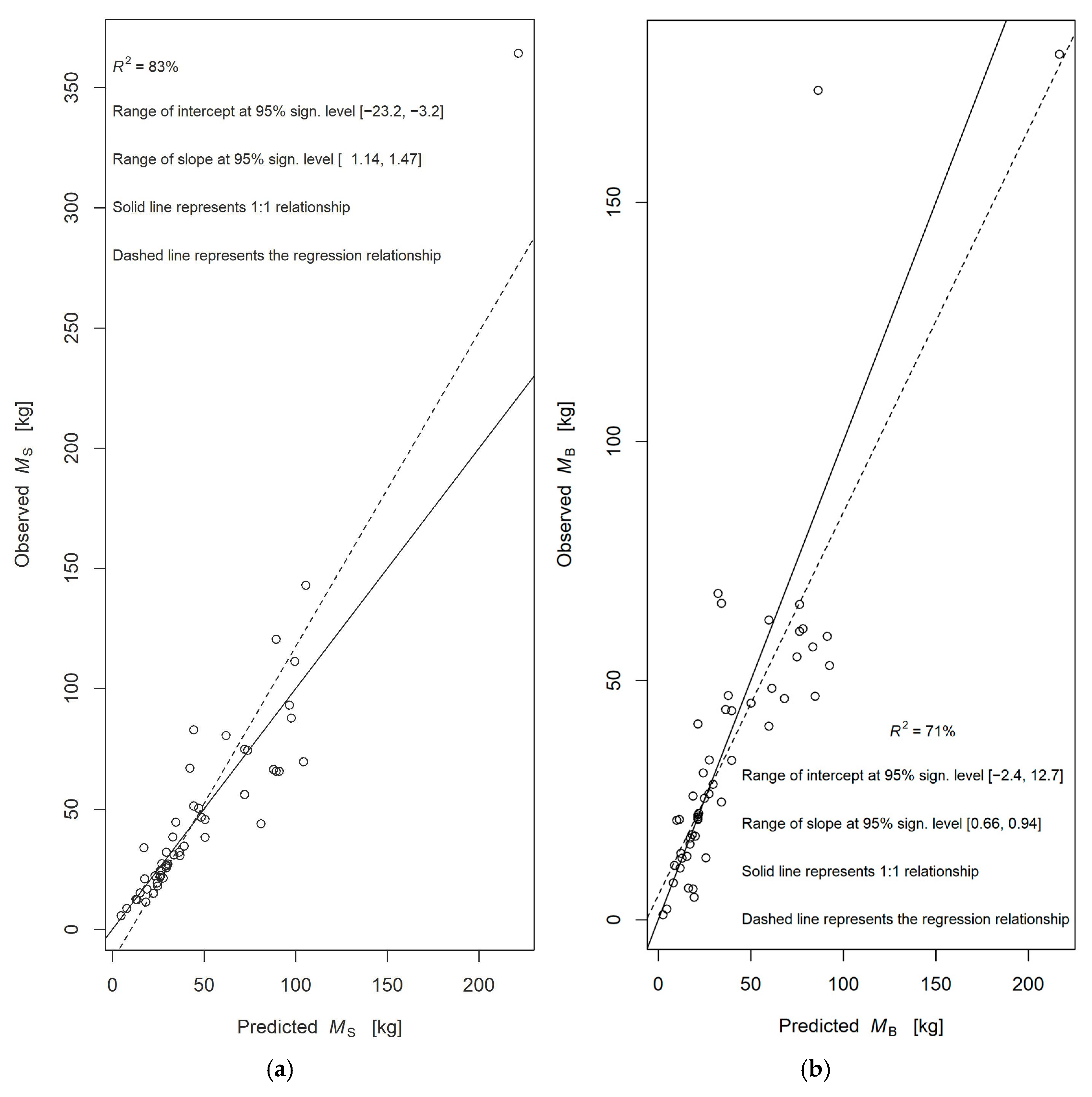
The “intrinsically nonlinear” regressions for different tree components are depicted in the Supplementary Materials (Figure S3), along with graphs illustrating the goodness-of-fit criteria. The estimates for the allometric exponent, the constant, and the fitted criteria for different components are reported in Table 3. The comparison of different allometric relationships predicting MS indicated that Equation (A14) in Appendix B better performed than its counterparts in terms of the White test criterion (13.21%, see in the Supplementary Materials Figure S3) and presented less profound “heavy-tailed” residuals in the Q–Q plot. The derived MS values explained more than 85% of the observed data, and PD was around 28% (see in the Supplementary Materials Figure S3A; Equation (A14)). Even though Equations (A15)–(A17) attained lower PD values (ca. 23%), the residuals presented high heteroskedasticity (White test < 5%).
For MB, Equation (A18) provided better results in terms of the White test criterion (Figure S3B in the Supplementary Materials) and PD value (Table 3), but the residuals were slightly positively skewed (Q–Q plot in Figure S3B in the Supplementary Materials). Finally, Equation (A24) was selected as the most appropriate to estimate MT for the studied trees (PD ca. 28%; White test > 5%; Q–Q plot near normality and predicted values explained more than 90% of the variability in the raw data).
In comparison to linear approaches, the analyzed nonlinear equations provided better predictions in terms of fitted criteria. For the stem component, PD ranged from 37.7 to 43.8% for linear regressions (Table 1; Equations (A1)–(A4)), while PD ranged from 22 to 30% for allometric relationships (Table 3; Equations (A13)–(A17)). For MB, linear approaches obtained PD values of more than 98% (Table 1; Equations (A5)–(A8)), while nonlinear regressions deviated, on average, around 45% (Table 3; Equations (A18)–(A22)). Allometric relationships provided better results for MT as well. Overall, the minimum AIC and BIC values were smaller for nonlinear models than for the linear regressions.
Log-transformed regressions performed equally well to nonlinear models, in terms of PD, AIC, and BIC values (compare Table 2 and Table 3), but nonlinear regressions outperformed log-linear models in explaining the variability of the observed biomass values. Comparing the regression analysis in Figure 2 to the linear model in Figure S3A in the Supplementary Materials for Equation (A17), we conclude that NLR explained 93.5% of the variability in MS, while log-linear regression explained 83%. Similar results were also obtained for the variability in MB. In Figure S3B in the Supplementary Materials for Equation (A18), the observed versus predicted values followed a 1:1 trend, while in Figure 2 the linear trend was statistically different from the 1:1 relationship.

3.5. NSUR Approach

Since Equations (A14) and (A18) were selected as the most appropriate equations to predict MS and MB, respectively, the biomass additivity structural system (Equation (3)) can be specified as:
M s M B M T = f S ( X S ,   0 ,   β S ,   β Β ) f B ( 0 ,   X B ,   β S ,   β Β ) f T ( X S ,   X B ,   β S ,   β Β ) + ε S ε B ε T
where f s = α 2 ( D 1.3 2 H ) b 2 , f B = α 6 D 1.3 b 6 (or equivalently Equations (A14) and (A18) in Appendix B),
and in turn, f T = α 2 ( D 1.3 2 H ) b 2 + α 6 D 1.3 b 6 .
The design matrices are presented as XS and XB and βS = [a2, b2]′, βB = [a6, b6]′.
The parameters in Equation (8) were estimated through the nlsur library in R [47]. Arguments in nlsur allow for inserting a weighted covariance matrix whose elements were estimated using Equation [21] in Parresol [30]. Even though the selected allometries for MB and MT did not present any heteroskedasticity trend, their residuals were highly correlated (0.46), so a weight function was used for each component to estimate the variance of the parameters. The procedure reported in Parresol ([29]; Section 1.1.5) was applied and the variance function for MS was found to be dependent on D−1.989, for MB on D−1.983, and for MT on D−2.001. To simplify the analysis, the weight functions for the three components were assumed to depend on D−2. The estimated coefficients in Table 4 and their standard errors corresponded to the NSUR model, which ensured the additivity property in biomass estimation (a1, b1 corresponded to the stem biomass model and a2, b2 corresponded to the branch model). Meanwhile, Figure 3 illustrates the expected M predicted values for each tree component and the associated 95% prediction intervals, as calculated via Equation (4a,b).
The NSUR predictions of the three components were improved (in terms of PD and Rse) in relation to the nonlinear regressions, while the estimated log-normal distribution of the predicted M values captured the “dispersion” of the raw datasets. For example, only 2–3 observed values fell beyond the 95% prediction intervals for MS, MB, and MT. More importantly, the derived NSUR results provided biologically sound M estimates via the constrained parameters property, as illustrated in the following example. Taking into consideration a sampled tree with D1.3 = 30.24 cm and H = 4.7 m, the predicted MS was 0.0657(30.242 × 4.7)0.8131 = 59.1 kg and the expected MB was 0.0589 × 30.242.0696 = 68.2 kg. Thus, the predicted MT was 59.1 + 68.2 = 127.3 kg, which coincides with the mean value in Figure 4 (plot at bottom-left). It is noted that this property holds true for all the collected data. On the other hand, the summation of the predictions from nonlinear regressions presented in Table 3 for MS (Equation (A14)) and MB (Equation (A18)) equaled 129.8 kg (61.8 + 68) and diverged from estimates derived from Equation (A24), MT = 0.3158(30.242 × 4.7)0.6998 = 110.2 kg.

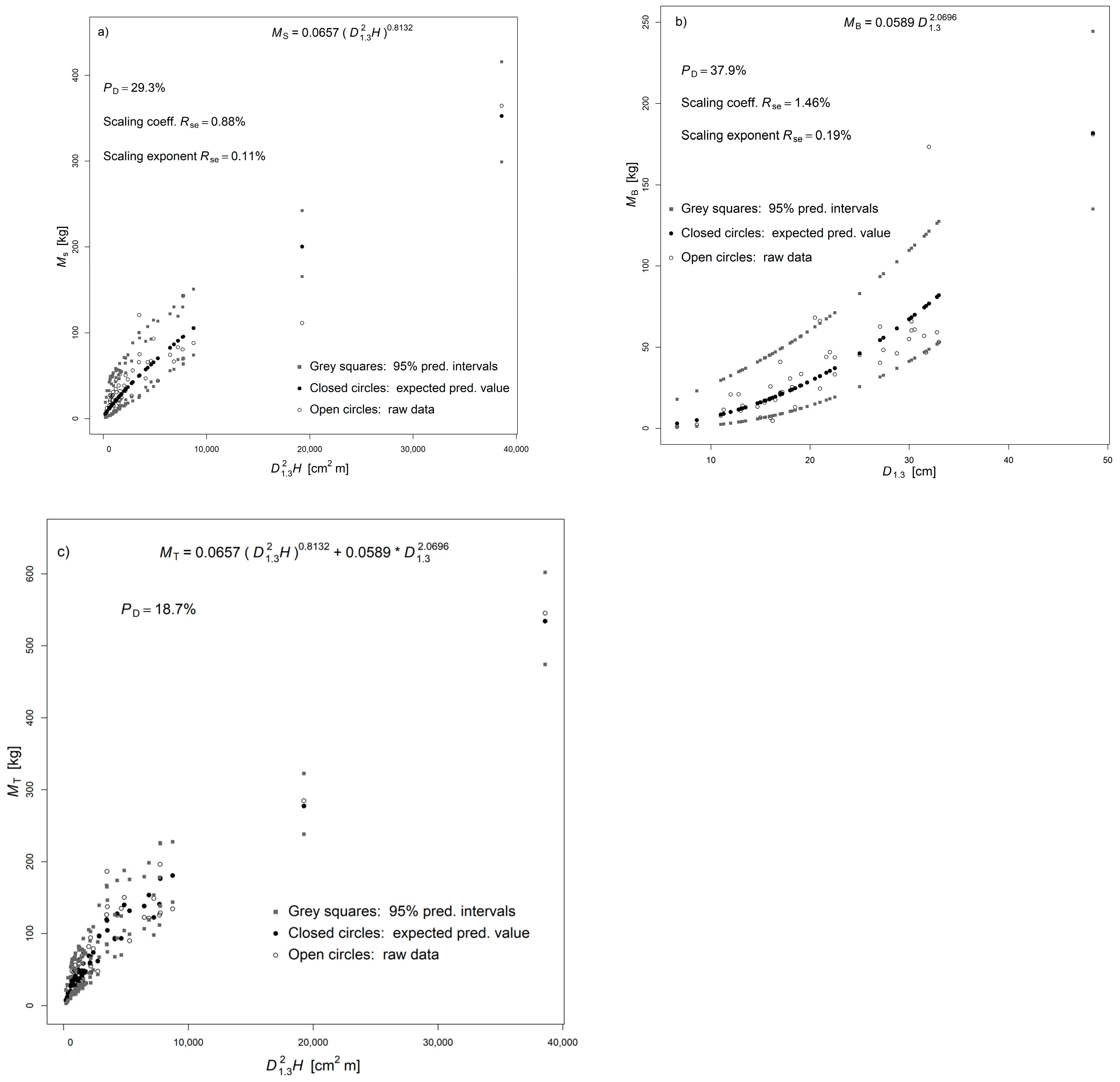
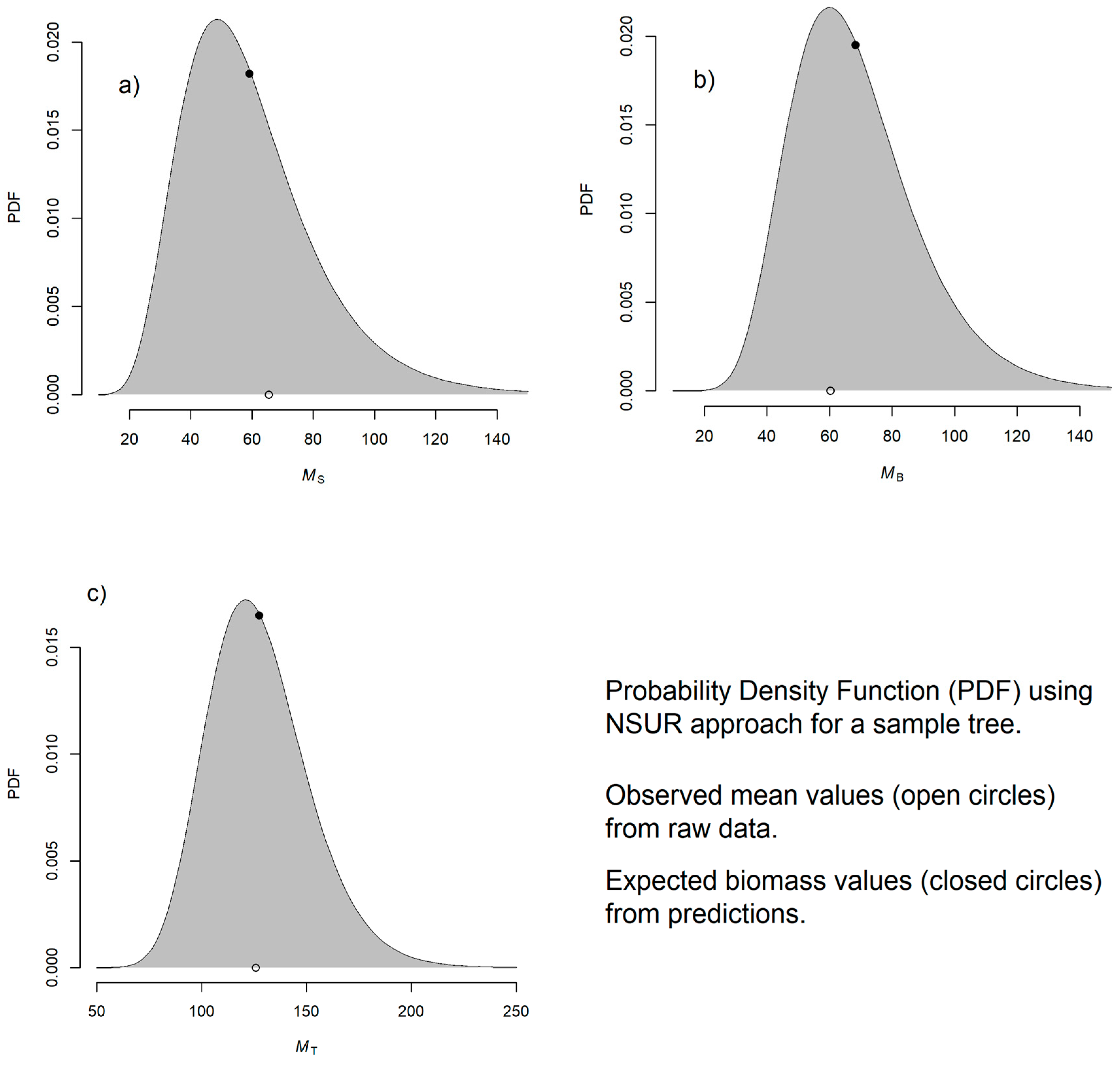
3.6. Implementing NSUR Approach

Estimation of predicted M values using the NSUR approach is a straightforward procedure. For example, let D1.3 = 20.7 cm and H = 6.1 m be the linear dimensions of a new sampled tree (which are actually the mean values of the sampled trees). The coefficient values in Table 4 can be applied to the new specimen, and the following predictions are derived:
MSn = 0.0657(20.72 × 6.1)0.8131 = 39.5 kg
MBn = 0.0589 × 20.72.0696 = 31.2 kg
MTn = 39.5 + 31.2 = 70.7 kg
The estimated variance of the predicted values from a specific equation is calculated via Equation (27) in Parresol [30] viz. S2 = f(b)′ Σb f(b), where f(b)′ is a row vector whose elements are the partial derivatives of the equation with respect to the parameters, and Σb is the covariance matrix of the parameters. Τhe standard error of the prediction, for the new tree, is given by Se = S2 + σ2Ν σΕ ψΕ, where σ2Ν and σΕ are estimated through Equations (26) and (32) in Parresol [30], respectively; ψΕ denotes the weight of the specific function for the new predictor value. The row vector of the partial derivatives of MSn with respect to the parameters, for the new tree, is the following:
fS(b)′ = [(D1.32 H)b2, a2(lnD1.3 + lnH) (D1.32 H)b2, 0, 0] = [600.84, 310.73, 0, 0]
and
Σ b = 3.36 × 10 7 5.01 × 10 7 2.08 × 10 7 9.48 × 10 7 5.01 × 10 7 7.53 × 10 7 3.16 × 10 7 1.4 × 10 6 2.08 × 10 7 3.16 × 10 7 7.43 × 10 7 3.43 × 10 6 9.48 × 10 7 1.4 × 10 6 3.43 × 10 6 1.59 × 10 5
as derived from the nlsur package, based on all the sampled trees.
Thus, for MSn, the estimated variance equals
Ss2 = fS(b)′ Σb fS(b) = 0.00669 kg2 and
σΕ = 0.565 kg2 cm2 and
ψΕ = 20.72 = 428.49 cm−2
The NSUR system variance for the structural equations and the specific dataset was estimated as σ2Ν = 0.9429 kg2.
In effect, the standard error of the MSn prediction for the given tree is Se = Ss2 + σ2Ν σΕ ψΕ = 0.00669 + 0.9429 × 0.565 × 428.49 = 228.48 kg2.
Assuming that M predictions follow a log-normal distribution (Section 2.2.5), Equation (4a,b) are applied and the prediction intervals for different tree components are the following:
for MSn [21.5–72.5 kg], for MBn [15.3–63.4 kg], and for MTn [48.3–103.4 kg].

3.7. Comparison to i–Tree Predictions

The predicted NSUR values were compared against i-Tree carbon estimates using the MyTree application [57], where the data characteristics for each individual sampled tree were entered. The results of this comparison are reported in the Supplementary Materials (Table S2). The MT values derived from NSUR predictions were divided by 2 to obtain carbon estimates. The predicted NSUR carbon value for each specimen was symbolized as Ni, and the corresponding carbon content was predicted by i-Tree as Ii. For each entry, the percentage difference (|1 − Ii/Ni| × 100) is also shown, providing a measure of how closely the i-Tree estimates align with NSUR predictions.
Overall, the mean deviation between NSUR and i-Tree predictions amounted to 134.36%. The range of deviation was 3.02% to 519.73%, with the highest value denoted for Ligustrum japonicum and the lowest for Ailanthus altissima.

4. Discussion

Very strong biomass allometries were derived from the studied urban trees, in spite of the genetic diversification of the specimens (individuals belonging to different taxa) and the intensified human-induced effects (pruning, soil compaction, vandalism, etc). Since the pioneering work of Nowak [58] on estimating CO2 in urban forests, no empirical scaling equations for predicting street tree biomass have been conducted so far, to the best of our knowledge. The obtained empirical equations in this study, developed using a pooled dataset of multiple species, represent one of the first attempts to estimate accumulated organic matter and CO2 assimilation for urban trees, with very high accuracy (in Figure 3 PD = 19% for MT). The models provided larger PD values for MS (ca. 30%) and MB (ca. 38%); the inclusion of several linear dimensions (D0.3, DC, HS) did not improve the accuracy of the predicted values. Additionally, there is a high correlation between the aforementioned variables, so by including them in the modelling process, confounding results might have been produced due to the multicollinearity property. At this point it should be emphasized that, contrary to forest trees, there was no relationship between H and D1.3 (see scatter plot in Figure 1) and therefore there was no issue of multicollinearity for model A14 (Appendix B). The frequent and intense human-induced effects on urban tree canopies may affect the relationship between H and D1.3. Introducing qualitative variables regarding the stature and the health status of urban tree crows in biomass allometries might have improved the accuracy of biomass predictions (specifically for MS and MB). However, since this is the first attempt to model size–shape scaling relationships in urban trees, such variables were not provisionally included in the sampling protocol. It is proposed that this type of dataset should be collected if these analyses will be pursued in future studies.
Apart from predicting the expected (average) tree biomass value for a single tree, variance prediction is equally important, so as to probabilistically estimate the range of the derived M values for a specific urban tree. The example presented in Section 3.6 is a straightforward approach to estimate 95% prediction intervals for NSUR models. The theoretical background and the statistical details are thoroughly explained in Parresol [29] and Parresol [30]. As illustrated in Figure 3, a very small proportion of the sampled trees fell beyond the prediction intervals, indicating the useability of this analysis in identifying the uncertainty level for estimating M values. It is pointed out that probability density function for M predictions is rarely reported for trees growing in forests. However, it is recommended to start reporting the upper and lower limits of predicted values, since variability around the mean is one of the most important properties of biological variables and strongly related to the quality assessment of the empirical studies.
Another issue of allometric relationships which is not gaining much attention in biomass studies is the additivity property of different tree components. The mathematical analysis required to build robust and efficient models free of additivity errors may have been too cumbersome for most of the researchers so far. However, the advent of freely available software and the exemplified approaches published in scientific articles and textbooks [29,30,35] remove the restrictions imposed by time-consuming and laborious calculations (or miscalculations). The additivity property of the sampled trees was modelled through Equation (8) and a very strong relationship for predicting MT was obtained (Figure 3), stressing the usefulness of this approach in predicting M.
Tree biomass allometries for forest and agroforest trees have also been examined under the Bayesian framework [59,60,61,62]. The full potential of Bayesian modelling can be initiated by the use of prior probability distributions of the parametric values, in Equation (1). Additionally, the uncertainty in M predictions may follow several formulations of error structure (multiplicative/additive), while information on statistical parameters from published allometries can be incorporated into a Bayesian context to improve M predictions [61,62]. However, since empirical biomass equations for urban trees have not been published so far, informative Bayesian modelling could not be developed for the studied trees. Having used the statistical values derived from trees growing in forested ecosystems, large deviations would have been derived [58,63]. Thus, only the classical (frequentist) approach was applied in this article to model the biomass of urban trees.
For comparative analysis, the i-Tree MyTree application [57] was utilized to evaluate carbon predictions against those derived from the NSUR model. A mean absolute percentage difference (PD) of 134.36% across all samples indicates a moderate to high level of variability between the models, underscoring the importance of refining predictive models for enhanced accuracy in carbon estimation. This observed variability aligns with findings from McHale et al. [13], who reported variances in biomass estimates up to 300% for individual urban trees compared to forest-based predictions, despite a reduction to 60% variability at larger scales. Similarly, Yoon et al. [14] noted substantial overestimation biases ranging from 68 to 427% when using equations developed for forest trees to predict urban biomass. These comparisons highlight how models not specifically tailored to urban trees can yield substantial predictive discrepancies, reinforcing the necessity of refining models to account for urban-specific conditions.
i-Tree’s tools for urban forest assessment serve as valuable benchmarks; however, the findings of this study underscore the necessity of refining predictive models to account for the unique characteristics of urban environments. As urban trees face distinct environmental stresses and management practices, specifically tailored models are critical to achieving more accurate carbon and biomass predictions. Past studies (e.g., Genet et al. [64]; Gourlet-Fleury et al. [65]) emphasize the importance of accounting for environmental variability, as tree growth differs significantly between urban and forested settings. When a species-specific equation is not available, i-Tree estimates biomass by averaging the results from equations of the same genus. If genus-specific equations are not available, i-Tree then applies the average of all broadleaf or coniferous tree equations, depending on the case [58,63]. This variability reinforces the necessity of context-specific approaches in biomass estimation, ensuring that urban forestry strategies will be informed by precise, empirically grounded data [8,66].
In future work, validating the developed models with new datasets is essential to assess the predictive accuracy and robustness across diverse urban tree species and varying urban conditions. This validation will enhance the model’s applicability and reliability in broader urban contexts, capturing the unique influences of urban environments on tree growth and carbon storage. While a single formula provides a generalized approach for urban tree biomass estimation, species-specific models have been widely developed, primarily for trees growing in non-mixed forested ecosystems. Future research should evaluate the trade-offs between generalized models for urban settings and species-specific models which have traditionally been applied to pure (single species) forest stands to optimize both accuracy and usability. The practical limitations of small sample sizes for certain species make species-specific equations less statistically reliable at this stage. The inclusion of multiple species in a single model improves statistical robustness and enhances applicability, particularly in urban environments where tree composition is often heterogeneous, and growth is shaped by artificial rather than natural selection pressures. Unlike trees in mixed forests, urban trees do not experience strong interspecies competition; instead, their biomass accumulation is affected by anthropogenic influences such as pruning, soil compaction, and air pollution. These factors contribute to growth patterns that may not strictly adhere to species-level differences, supporting the need for an integrated allometric approach. Additionally, applying these models specifically within the Attica region offers a valuable opportunity to inform urban forest management and policy initiatives. Such regional applications could provide insights that support sustainable urban planning and contribute to broader efforts in carbon management and climate resilience. This localized application may also serve as a framework for extending the model’s utility to other urban areas with similar ecological and environmental characteristics, further reinforcing its value as a tool for urban forestry research and practice.

5. Conclusions

This study contributes to the growing body of knowledge on urban tree biomass estimation by developing and validating allometric models that are sensitive to the distinct growth patterns and environmental pressures of urban settings. Integrating these findings into urban planning frameworks offers a pathway to optimizing green space design for maximal environmental benefits, while also providing urban policymakers with actionable insights into the carbon sequestration potential of urban trees. By quantifying aboveground biomass and addressing the additivity property, this research supports more accurate assessments of carbon storage across varied urban ecosystems, advancing our understanding of biomass dynamics in urban environments. Given the structural and physiological diversity among species, future refinements in biomass estimation may benefit from approaches that account for interspecies variation while maintaining broad applicability in urban forestry.

Supplementary Materials

The following supporting information can be downloaded at: https://www.mdpi.com/article/10.3390/f16030466/s1, Figure S1: Derived linear regressions for different tree components: (A) stem biomass (Models A1–A4); (B) branch biomass (Models A5–A8); (C) total biomass (Models A9–A12); Figure S2: goodness-of-fit statistics and visual inspection of models’ performance for different tree components: (A) stem biomass (Models A1–A4); (B) branch biomass (Models A5–A8); (C) total biomass (Models A9–A12); Figure S3: Nonlinear regression allometries and graphs depicting goodness-of-fit criteria for different tree components: (A) stem biomass (Equations A13–A17); (B) branch biomass (Equations A18–A22); (C) total biomass (Equations A23–A27); Table S1: Descriptive Statistics for the fifty-two sampled trees, including diameter, height, and crown length measurements; Table S2: Comparison of carbon content predictions for sampled trees using NSUR and i-Tree models.

Author Contributions

Conceptualization, M.D. and D.Z.; methodology, M.D. and D.Z.; software, M.D. and D.Z.; validation, M.D. and D.Z.; formal analysis, M.D. and D.Z.; investigation, M.D. and D.Z.; resources, M.D. and D.Z.; data curation, M.D. and D.Z.; writing—original draft preparation, M.D. and D.Z.; writing—review and editing, M.D. and D.Z.; visualization, M.D. and D.Z.; supervision, M.D. and D.Z.; project administration, M.D. and D.Z. All authors have read and agreed to the published version of the manuscript.

Funding

This research received no external funding.

Data Availability Statement

The data supporting the findings of this study are available upon request from the first author.

Acknowledgments

The support from the Institute of Mediterranean Forest Ecosystems and the Municipality of Athens, Department of Greenery & Urban Fauna, for this work is greatly appreciated.

Conflicts of Interest

The authors declare no conflicts of interest.

Abbreviations

The following abbreviations are used in this manuscript:
MTree biomass
MTTotal aboveground dry biomass (MS + MB) in kg
MSStem dry biomass in kg
MBBranches’ dry biomass in kg
HTree height (m)
HSStem height (m)
HCCrown height (m)
CLCrown length in centimeters (cm)
D0.30Tree diameter at a height of 0.30 above the ground in centimeters (cm)
D1.30Diameter at breast height, at a height of 1.30 above the ground in centimeters (cm)
DCDiameter at the base of the crown in centimeters (cm)
B0.3Basal area at 0.3 meters aboveground (m2)
B1.3Basal area at 1.3 meters aboveground (m2)
BCBasal area at the base of the crown (m2)

Appendix A

MS = s1H(B0.3 + BC)/2 + s2
MS = s3HS (B0.3 + BC)/2 + s4
MS = s5H(B0.3 + 4B1.3 + BC)/6 + s6
MS = s7HS(B0.3 + 4B1.3 + BC)/6 + s8
MB = s1H(B0.3 + BC)/2 + s2
MB = s3 HS(B0.3 + BC)/2 + s4
MB = s5H(B0.3 + 4B1.3 + BC)/6 + s6
MB = s7HS(B0.3 + 4B1.3 + BC)/6 + s8
MT = s9H(B0.3 + BC)/2 + s10
MT = s11HS(B0.3 + BC)/2 + s12
MT = s13H(B0.3 + 4B1.3 + BC)/6 + s14
MT = s15 HS(B0.3 + 4B1.3 + BC)/6 + s15

Appendix B

M s = α 1 D 1.3 b 1 + ε
M s = α 2 ( D 1.3 2 H ) b 2 + ε
M s = α 3 D 1.3 b 3 H c 3 + ε
M s = α 4 ( D 1.3 2 H s ) b 4 + ε
M s = α 5 ( D c 2 H s ) b 5 + ε
M B = α 6 D 1.3 b 6 + ε
M B = α 7 ( D 1.3 2 H ) b 7 + ε
M B = α 8 D 1.3 b 8 H c 8 + ε
M B = α 9 ( D 1.3 2 H c ) b 9 + ε
M B = α 10 ( D 1.3 b 10 H c ) c 10 + ε
M T = α 11 D 1.3 b 11 + ε
M T = α 12 ( D 1.3 2 H ) b 12 + ε
M T = α 13 D 1.3 b 13 H c 13 + ε
M T = α 14 ( D 1.3 b 14 H s ) b 14 + ε
M T = α 15 ( D 1.3 b 15 H c ) c 15 + ε

References

  1. McPherson, E.G.; Simpson, J.R. Carbon Dioxide Reduction Through Urban Forestry: Guidelines for Professional and Volunteer Tree Planters; U.S. Department of Agriculture, Forest Service, Pacific Southwest Research Station: Albany, CA, USA, 1999. [CrossRef]
  2. Pataki, D.E.; Alig, R.J.; Fung, A.S.; Golubiewski, N.E.; Kennedy, C.A.; Mcpherson, E.G.; Nowak, D.J.; Pouyat, R.V.; Romero Lankao, P. Urban ecosystems and the North American carbon cycle. Glob. Change Biol. 2006, 12, 2092–2102. [Google Scholar] [CrossRef]
  3. McPherson, E.G.; van Doorn, N.S.; Peper, P.J. United States Department of Agriculture Urban Tree Database and Allometric Equations; General Technical Report; PSW-GTR-235; U.S. Department of Agriculture: Albany, CA, USA, 2016. [CrossRef]
  4. Pretzsch, H.; Forrester, D.I.; Rötzer, T. Representation of species mixing in forest growth models: A review and perspective. Ecol. Model. 2015, 313, 276–292. [Google Scholar] [CrossRef]
  5. Song, X.P.; Lai, H.R.; Wijedasa, L.S.; Tan, P.Y.; Edwards, P.J.; Richards, D.R. Height-diameter allometry for the management of city trees in the tropics. Environ. Res. Lett. 2020, 15, 114017. [Google Scholar] [CrossRef]
  6. Nowak, D.J. Understanding i-Tree; U.S. Department of Agriculture, Forest Service, Northern Research Station: Madison, WI, USA, 2021. [CrossRef]
  7. i-Tree Tools. Available online: https://www.itreetools.org/ (accessed on 23 June 2024).
  8. Lin, J.; Kroll, C.N.; Nowak, D.J.; Greenfield, E.J. A review of urban forest modeling: Implications for management and future research. Urban For. Urban Green. 2019, 43, 126366. [Google Scholar] [CrossRef]
  9. Pinkard, E.A.; Beadle, C.L. Aboveground biomass partitioning and crown architecture of Eucalyptus nitens following green pruning. Can. J. For. Res. 1998, 28, 1419–1428. [Google Scholar] [CrossRef]
  10. Bandara, G.D.; Whitehead, D.; Mead, D.J.; Moot, D.J. Effects of pruning and understorey vegetation on crown development, biomass increment and above-ground carbon partitioning in Pinus radiata D. Don trees growing at a dryland agroforestry site. For. Ecol. Manag. 1999, 124, 241–254. [Google Scholar] [CrossRef]
  11. Kramer, P.J.; Kozlowski, T.T. Physiology of Woody Plants; Academic Press: New York, NY, USA, 1979. [Google Scholar]
  12. Rhoades, R.W.; Stipes, R.J. Growth of trees on the Virginia Tech campus in response to various factors. Arboric. Urban For. 1999, 25, 211–217. [Google Scholar] [CrossRef]
  13. McHale, M.R.; Burke, I.C.; Lefsky, M.A.; Peper, P.J.; McPherson, E.G. Urban forest biomass estimates: Is it important to use allometric relationships developed specifically for urban trees? Urban Ecosyst. 2009, 12, 95–113. [Google Scholar] [CrossRef]
  14. Yoon, T.K.; Park, C.-W.; Lee, S.J.; Ko, S.; Kim, K.N.; Son, Y.; Lee, K.H.; Oh, S.; Lee, W.-K.; Son, Y. Allometric equations for estimating the aboveground volume of five common urban street tree species in Daegu, Korea. Urban For. Urban Green. 2013, 12, 344–349. [Google Scholar] [CrossRef]
  15. Yang, M.; Zhou, X.; Liu, Z.; Li, P.; Tang, J.; Xie, B.; Peng, C. A Review of General Methods for Quantifying and Estimating Urban Trees and Biomass. Forests 2022, 13, 616. [Google Scholar] [CrossRef]
  16. Pillsbury, N.H.; Reimer, J.L. Tree Volume Equations for 10 Urban Species in California 1; U.S. Department of Agriculture, Forest Service: Albany, CA, USA, 1997.
  17. Huxley, J.S. Problems of Relative Growth; Methuen Publishing: London, UK, 1932. [Google Scholar]
  18. Broad, L.R. AIIometry and Growth. For. Sci. 1998, 44, 458–464. [Google Scholar]
  19. Jenkins, J.C.; Chojnacky, D.C.; Heath, L.S.; Birdsey, R.A. National-Scale Biomass Estimators for United States Tree Species. For. Sci. 2003, 49, 12–35. [Google Scholar] [CrossRef]
  20. Návar, J. Allometric equations for tree species and carbon stocks for forests of northwestern Mexico. For. Ecol. Manag. 2009, 257, 427–434. [Google Scholar] [CrossRef]
  21. Pilli, R.; Anfodillo, T.; Carrer, M. Towards a functional and simplified allometry for estimating forest biomass. For. Ecol. Manag. 2006, 237, 583–593. [Google Scholar] [CrossRef]
  22. Ter-Mikaelian, M.T.; Korzukhin, M.D. Biomass equations for sixty-five North American tree species. For. Ecol. Manag. 1997, 97, 1–24. [Google Scholar] [CrossRef]
  23. West, G.B.; Brown, J.H.; Enquist, B.J. A general model for the origin of allometric scaling laws in biology. Science 1997, 276, 122–126. [Google Scholar] [CrossRef] [PubMed]
  24. Zianis, D. Predicting mean aboveground forest biomass and its associated variance. For. Ecol. Manag. 2008, 256, 1400–1407. [Google Scholar] [CrossRef]
  25. Zianis, D.; Muukkonen, P.; Mäkipää, R.; Mencuccini, M. Biomass and Stem Volume Equations for Tree Species in Europe. Silva Fennica Monographs 4; Finnish Society of Forest Science, Finnish Forest Research Institute: Helsinki-Uusimaa, Finland, 2005. [Google Scholar] [CrossRef]
  26. Zianis, D.; Mencuccini, M. Aboveground net primary productivity of a beech (Fagus moesiaca) forest: A case study of Naousa forest, northern Greece. Tree Physiol. 2005, 25, 713–722. [Google Scholar] [CrossRef]
  27. Zianis, D.; Mencuccini, M. Aboveground biomass relationships for beech (Fagus moesiaca Cz.) trees in Vermio Mountain, Northern Greece, and generalised equations for Fagus sp. Ann. For. Sci. 2003, 60, 439–448. [Google Scholar] [CrossRef]
  28. Payandeh, B. Choosing Regression Models for Biomass Prediction Equations. For. Chron. 1981, 57, 229–232. [Google Scholar] [CrossRef]
  29. Parresol, B.R. Assessing Tree and Stand Biomass: A Review with Examples and Critical Comparisons. For. Sci. 1999, 45, 573–593. [Google Scholar] [CrossRef]
  30. Parresol, B.R. Additivity of nonlinear biomass equations. Can. J. For. Res. 2001, 31, 865–878. [Google Scholar] [CrossRef]
  31. Sanquetta, C.R.; Netto, S.P.; Corte, A.P.D.; Rodrigues, A.L.; Behling, A.; Sanquetta, M.N.I. Quantifying biomass and carbon stocks in oil palm (Elaeis guineensis Jacq.) in Northeastern Brazil. Afr. J. Agric. Res. 2015, 10, 4067–4075. [Google Scholar] [CrossRef]
  32. Kozak, A. Methods for Ensuring Additivity of Biomass Components by Regression Analysis. For. Chron. 1970, 46, 402–404. [Google Scholar] [CrossRef]
  33. Reed, D.D.; Green, E.J. A method of forcing additivity of biomass tables when using nonlinear models. Can. J. For. Res. 1985, 15, 1184–1187. [Google Scholar] [CrossRef]
  34. Zellner, A. An Efficient Method of Estimating Seemingly Unrelated Regressions and Tests for Aggregation Bias. J. Am. Stat. Assoc. 1962, 57, 348–368. [Google Scholar] [CrossRef]
  35. Greene, W.H. Econometric Analysis, 4th ed.; Prentice Hall: Upper Saddle River, NJ, USA, 2000. [Google Scholar]
  36. Parresol, B.R. Modeling Multiplicative Error Variance: An Example Predicting Tree Diameter from Stump Dimensions in Baldcypress. For. Sci. 1993, 39, 676–679. [Google Scholar] [CrossRef]
  37. Hellenic Statistical Authority. Census 2021 GR. 2021. Available online: https://www.statistics.gr/2011-census-pop-hous (accessed on 25 June 2024).
  38. Municipality of Athens. Part I of the Climate Action Plan. 2022. Available online: https://www.cityofathens.gr/wp-content/uploads/2022/08/schedio-gia-tin-klimatiki-allagi-9-6-2022.pdf (accessed on 25 June 2024).
  39. World Meteorological Organization’s World Weather and Climate Extremes Archive. Available online: https://wmo.asu.edu/content/wmo-region-vi-europe-continent-only-highest-temperature (accessed on 25 June 2024).
  40. Hellenic National Meteorological Service. Available online: https://www.emy.gr/ (accessed on 15 January 2025).
  41. Pinheiro, J.C.; Bates, D.M. Mixed-Effects Models in S and S-PLUS; Springer: Berlin/Heidelberg, Germany, 2000. [Google Scholar] [CrossRef]
  42. Baskerville, G.L. Use of logarithmic regression in the estimation of plant biomass. Can. J. For. Serv. 1972, 2, 49–53. [Google Scholar] [CrossRef]
  43. Beauchamp, J.J.; Olson, J.S. Corrections for Bias in Regression Estimates After Logarithmic Transformation. Ecology 1973, 54, 1403–1407. [Google Scholar] [CrossRef]
  44. Sprugel, D.G. Correcting for Bias in Log-Transformed Allometric Equations. Ecology 1983, 64, 209–210. [Google Scholar] [CrossRef]
  45. Yandle, D.O.; Wiant, H.V. Estimation of plant biomass based on the allometric equation. Can. J. For. Res. 1981, 11, 833–834. [Google Scholar] [CrossRef]
  46. Wiant, H.V.J.; Harner, E.J. Percent bias and standard error in logarithmic regression. For. Sci. 1979, 25, 167–168. [Google Scholar]
  47. JanMarvin/nlsur: Estimating Nonlinear Least Squares for Equation Systems Version 0.8 from GitHub. Available online: https://rdrr.io/github/JanMarvin/nlsur/ (accessed on 1 December 2024).
  48. Mehtätalo, L.; Lappi, J. Forest Biometrics with Examples in R Contents; CRC: Boca Raton, FL, USA, 2020. [Google Scholar]
  49. Limpert, E.; Stahel, W.A.; Abbt, M. Log-normal distributions across the sciences: Keys and clues. Bioscience 2001, 51, 341–352. [Google Scholar] [CrossRef]
  50. Thomopoulos, N.T.; Johnson, A.C. Tables And Characteristics of the Standardized Lognormal Distribution. Proc. Decis. Sci. Inst. 2003, 103, 1031–1036. [Google Scholar]
  51. Ezekiel, M.; Fox, K.A. Methods of Correlation and Regression Analysis: Linear and Curvilinear; John Wiley and Sons Inc.: Taipei, Taiwan, 1959. [Google Scholar]
  52. Furnival, G. An index for comparing equations used in constructing volume tables. For. Sci. 1961, 7, 337–341. [Google Scholar]
  53. Schreuder, H.T.; Swank, W.T. A comparison of several statistical models in forest biomass and surface area estimation. In Forest Biomass Studies, IUFRO, Section 25: Yield and Growth. Life Sci. and Agric. Exp. Stn., Univ. Maine. Orono, ME, USA; Young, H.E., Ed.; Springer: Berlin/Heidelberg, Germany, 1971; pp. 125–138. [Google Scholar]
  54. Albini, F.A.; Brown, J.K. Predicting Slash Depth for Fire Modeling; Reserch Paper; INT-RP-206; USDA Forest Service, Intermountain Forest and Range Experiment Station: Ogden, UT, USA, 1978.
  55. Sileshi, G.W. A critical review of forest biomass estimation models, common mistakes and corrective measures. For. Ecol. Manag. 2014, 329, 237–254. [Google Scholar] [CrossRef]
  56. The R Project for Statistical Computing. Available online: https://www.r-project.org/ (accessed on 1 October 2024).
  57. MyTree Tool. Available online: https://mytree.itreetools.org/#/ (accessed on 11 November 2024).
  58. Nowak, D.J. Understanding the Structure of Urban Forests. J. For. 1994, 92, 42–46. [Google Scholar] [CrossRef]
  59. Dutcă, I.; Zianis, D.; Petrițan, I.C.; Bragă, C.I.; Ștefan, G.; Yuste, J.C.; Petrițan, A.M. Allometric biomass models for european beech and silver fir: Testing approaches to minimize the demand for site-specific biomass observations. Forests 2020, 11, 1136. [Google Scholar] [CrossRef]
  60. Zapata-Cuartas, M.; Sierra, C.A.; Alleman, L. Probability distribution of allometric coefficients and Bayesian estimation of aboveground tree biomass. For. Ecol. Manag. 2012, 277, 173–179. [Google Scholar] [CrossRef]
  61. Zianis, D.; Spyroglou, G.; Tiakas, E.; Radoglou, K.M. Bayesian and classical models to predict aboveground tree biomass allometry. For. Sci. 2016, 62, 247–259. [Google Scholar] [CrossRef]
  62. Zianis, D.; Pantera, A.; Papadopoulos, A.; Losada, M.R.M. Bayesian and classical biomass allometries for open grown valonian oaks (Q. ithaburensis subs. macrolepis L.) in a silvopastoral system. Agrofor. Syst. 2017, 93, 241–253. [Google Scholar] [CrossRef]
  63. Aguaron, E.; McPherson, E.G. Comparison of methods for estimating carbondioxide storage by sacramento’s urban forest. In Carbon Sequestration in Urban Ecosystems; Springer: Dordrecht, The Netherlands, 2012; pp. 44–71. [Google Scholar] [CrossRef]
  64. Genet, A.; Wernsdörfer, H.; Jonard, M.; Pretzsch, H.; Rauch, M.; Ponette, Q.; Nys, C.; Legout, A.; Ranger, J.; Vallet, P.; et al. Ontogeny partly explains the apparent heterogeneity of published biomass equations for Fagus sylvatica in central Europe. For. Ecol. Manag. 2011, 261, 1188–1202. [Google Scholar] [CrossRef]
  65. Gourlet-Fleury, S.; Rossi, V.; Rejou-Mechain, M.; Freycon, V.; Fayolle, A.; Saint-André, L.; Cornu, G.; Gérard, J.; Sarrailh, J.-M.; Flores, O.; et al. Environmental filtering of dense-wooded species controls above-ground biomass stored in African moist forests. J. Ecol. 2011, 99, 981–990. [Google Scholar] [CrossRef]
  66. Lin, J.; Kroll, C.N.; Nowak, D.J. An uncertainty framework for i-Tree eco: A comparative study of 15 cities across the United States. Urban For. Urban Green. 2021, 60, 127062. [Google Scholar] [CrossRef]
Figure 1. Summary scatterplots for MT, MS, MB, D0.30, D1.30, DC, and H across the pooled dataset (MT: total aboveground dry biomass, MS: stem dry biomass, MB: branches dry biomass, D0.30: tree diameter at a height of 0.30 m above the ground in centimeters (cm), D1.30: diameter at breast height, at a height of 1.30 m above the ground in centimeters (cm), DC: the diameter at the base of the crown in centimeters (cm), H: the total height of the tree in meters (m).
Forests 16 00466 g001
Figure 2. Linear regression statistics from 52 sampled trees across 10 different species, showing observed versus predicted values for (a) stem and (b) branch biomass.
Forests 16 00466 g002
Figure 3. Expected biomass values (closed circles) for the following tree component: (a) stem biomass (MS); (b) branch biomass (MB); (c) total biomass (MT) along with the associated 95% prediction intervals (grey squares), calculated using Equation (4a,b).
Forests 16 00466 g003
Figure 4. Predicted biomass values for the following tree component: (a) stem biomass (MS); (b) branch biomass (MB); (c) total biomass (MT), using NSUR approach based on nonlinear regressions for a sample tree (D1.3 = 30.24 cm, H = 4.7 m), highlighting the consistency of the Probability Density Function (PDF) from NSUR estimates (closed circles represent the mean predicted value) and the observed mean values (open circles).
Forests 16 00466 g004
Table 1. Linear regression statistics for stem, branch, and total aboveground biomass regressions in the form Y = a + bX (see Appendix A). The number of sampled trees is 52 belonging to 10 different species. R2: the coefficient of determination; s.e.: the standard errors of the estimates at 95% significance level; % s.e.: computed with Equation (7); PD (%): computed with Equation (6); RMSE: root mean square error; Akaike information criterion (AIC) and Bayesian information criterion (BIC) allow for model comparison, with lower values indicating a better fit.
ComponentEq.abs.e. (a)s.e. (b)Rse (a) %Rse (b) %PD (%)AICBICR2RMSE
StemA118.260893.01223.00944.712316.485.0738.5445.4522451.18820.8917.98
A218.6670249.92682.752011.540014.744.6243.8435.1883440.92430.9016.55
A318.7013103.16663.08655.396316.505.2337.7448.0563453.79240.8818.49
A418.5975285.66342.488911.840513.384.1440.3425.0899430.82590.9215.00
BranchA518.912052.29613.13454.908216.579.39103.8449.5247455.26070.6918.73
A621.3903122.59193.825416.041317.8813.09123.7468.1231473.85920.5423.00
A718.235361.04932.75004.807915.087.8898.6436.5118442.24780.7616.48
A820.9650143.67693.655117.388417.4312.1119.9463.5180469.25400.5822.02
TotalA937.1729145.30864.98147.800113.45.3747.6495.8484501.58450.8136.44
A1040.0575372.51856.059725.410415.136.8256.6514.1221519.85820.9026.44
A1136.9366164.21644.41187.713511.944.745.5483.7824489.51850.8433.49
A1239.5627429.34035.557926.441014.056.1653.6505.4290511.16500.8729.76
Table 2. Regression equations of the form Y = ln a + bX. The number of sampled trees is 52. R2: the coefficient of determination; s.e.: the standard errors of the estimates at 95% significance level; % s.e.: computed with Equation (7); SEE: standard error of the estimate; PD (%): computed with Equation (6); SSE: sum of squared errors; RMSE: root mean square error; Akaike Information Criterion (AIC) and Bayesian Information Criterion (BIC) values correspond to the original datasets and not on the log-transformed data; CF: the correction factor; %bias: computed with Equation (2b); S: computed with the Equation (5); MT: total aboveground dry biomass; MS: stem dry biomass; MB: branches dry biomass; D1.30: diameter at breast height, at a height of 1.30 above the ground in centimeters (cm).
YXlnabs.e. (a)s.e. (b)Rse (a) %Rse (b) %SEECF% bias% s.e.SSES
lnMSlnD1.3−2.09951.92310.29190.097813.905.090.26581.033.4618.9531,0390.79
lnMBlnD1.3−3.30092.20940.50070.167915.177.600.45591.109.8733.0919,706.170.67
lnMTlnD1.3−1.75981.99680.28330.09516.104.760.2581.033.2718.3955,240.980.85
YXPD (%)AICBICR2RMSE
lnMSlnD1.321.06387.20391.520.8924.43161
lnMBlnD1.340.9406.48413.250.7819.46702
lnMTlnD1.319.93442.13450.20.932.59336
Table 3. The estimates for the allometric exponent, the constant, and the fitted criteria for different components. Formulae of the equations in Appendix B.
ComponentEq.abcRse (a) %Rse (b) %Rse (c) %PD (%)AICBIC
StemA130.01022.6833-42.644.41-29.8450.5351456.3888
A140.11480.7518-37.245.17-27.7467.9970473.8508
A150.02792.20990.300740.436.4926.2323.3440.5869448.3919
A160.23970.7598-18.052.76-23.2415.7359421.5897
A170.22350.7655-19.662.97-21.7424.1670430.0208
BranchA180.08191.9719-58.388.54-40.8453.9460459.7997
A190.23510.6354-31.835.38-56.5422.3186428.1724
A200.22771.29110.618938.3910.3313.9155.7424.2816432.0866
A210.16440.7052-28.534.53-49.0404.3647410.2184
A220.20301.29300.804833.038.339.1152.2404.3980412.2030
TotalA230.05142.3688-41.034.89-21.0505.2491511.1028
A240.31590.6999-25.433.84-28.8487.1642493.0180
A250.16261.76160.445928.205.6313.1719.6471.6368479.4417
A260.26991.75240.428536.657.0217.8120.8482.3682490.1731
A270.12351.85960.503427.214.8612.1119.2466.5848474.3897
Table 4. Estimated coefficient values and standard errors from NSUR analysis, including the estimated coefficients, standard errors (s.e.), z-values, and p-values for each parameter (*** indicates a high level of statistical significance).
CoefficientEstimates.e.z-Valuep-Value
a10.06572460.0005797113.39 < 2 × 10 16 ***
b10.81315150.0008683936.52 < 2 × 10 16 ***
a20.05894740.000862368.36 < 2 × 10 16 ***
b22.06962030.0039958517.95 < 2 × 10 16 ***
Disclaimer/Publisher’s Note: The statements, opinions and data contained in all publications are solely those of the individual author(s) and contributor(s) and not of MDPI and/or the editor(s). MDPI and/or the editor(s) disclaim responsibility for any injury to people or property resulting from any ideas, methods, instructions or products referred to in the content.

