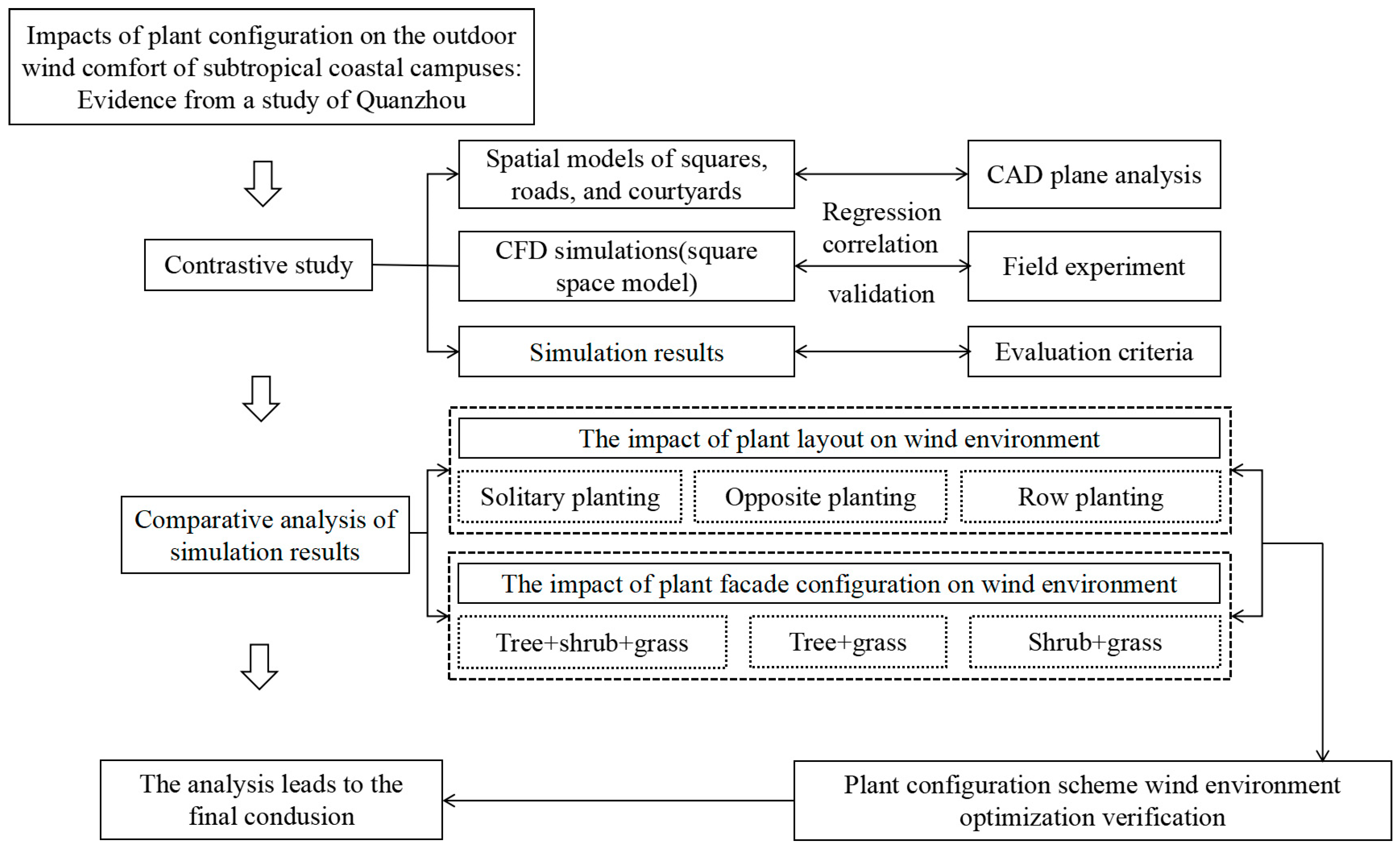
2.4.2. Details of Wind Environment Experiment and Simulations
- (1)
Measured Points Selection
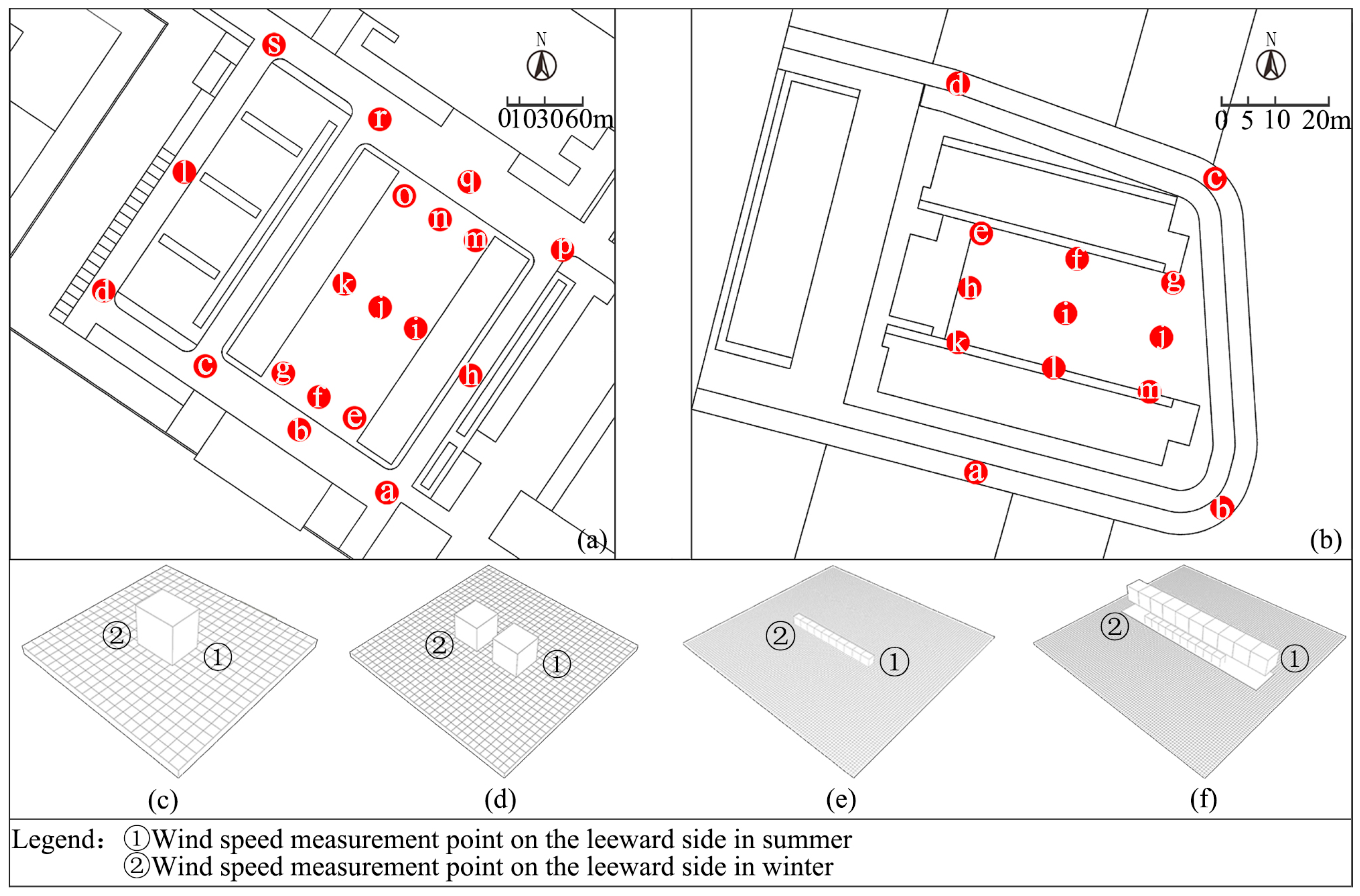
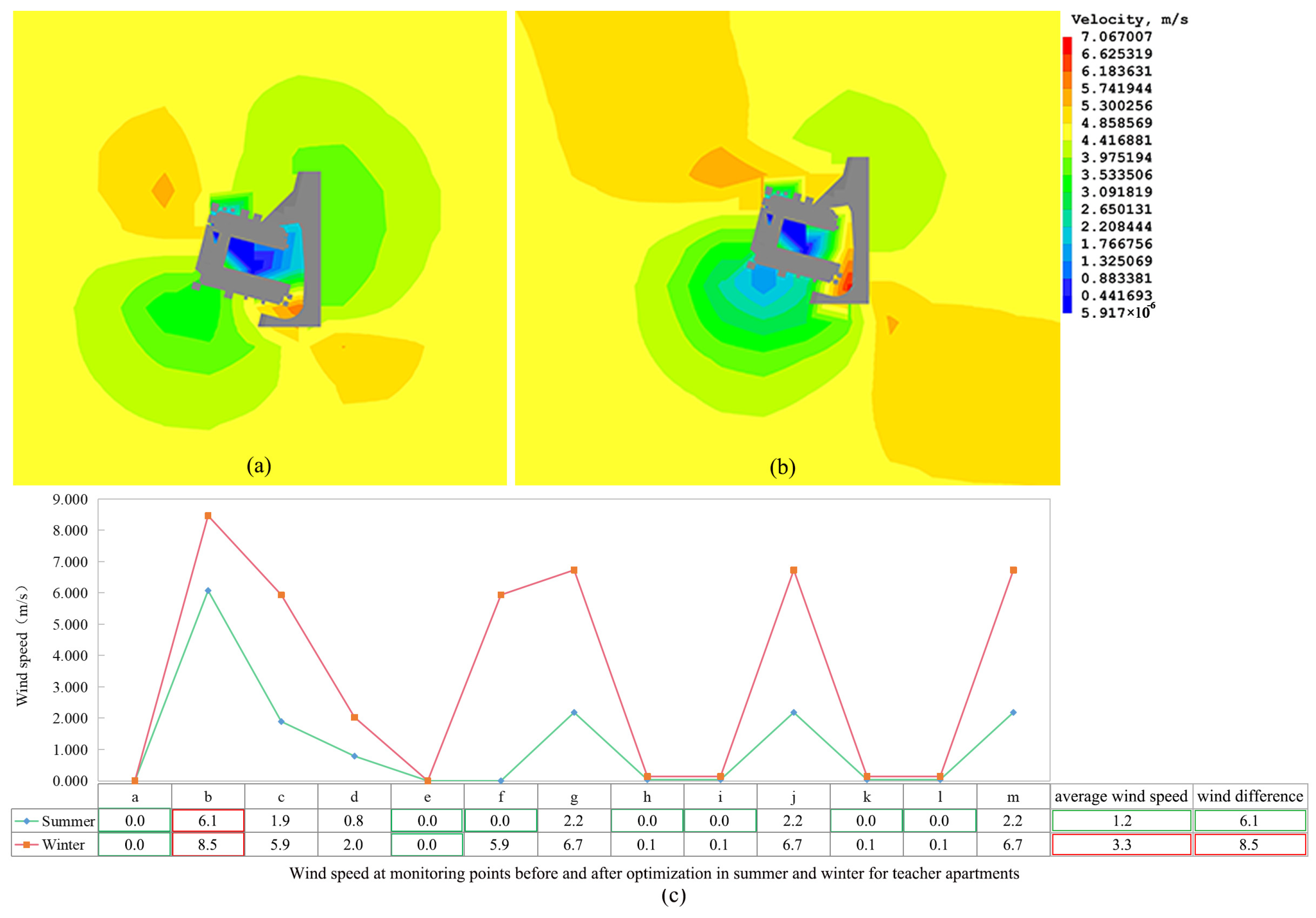
CFD was used to simulate the wind environment at the main gate square of the Donghai Campus of Quanzhou Normal University in order to clarify the horizontal flow field division in the outdoor area and determine the measurement points for the summer and winter wind conditions. Representative wind speed detection points were chosen according to the distinct flow patterns generated by natural winds during the summer and winter as they interact with the primary entrance square, individual building courtyards, and varied plant configurations: ① In terms of outdoor space, the main entrance square space in Zone A and the courtyard space of individual buildings in Zone E were selected, and 19 points most commonly involved in crowd activities in the square space (
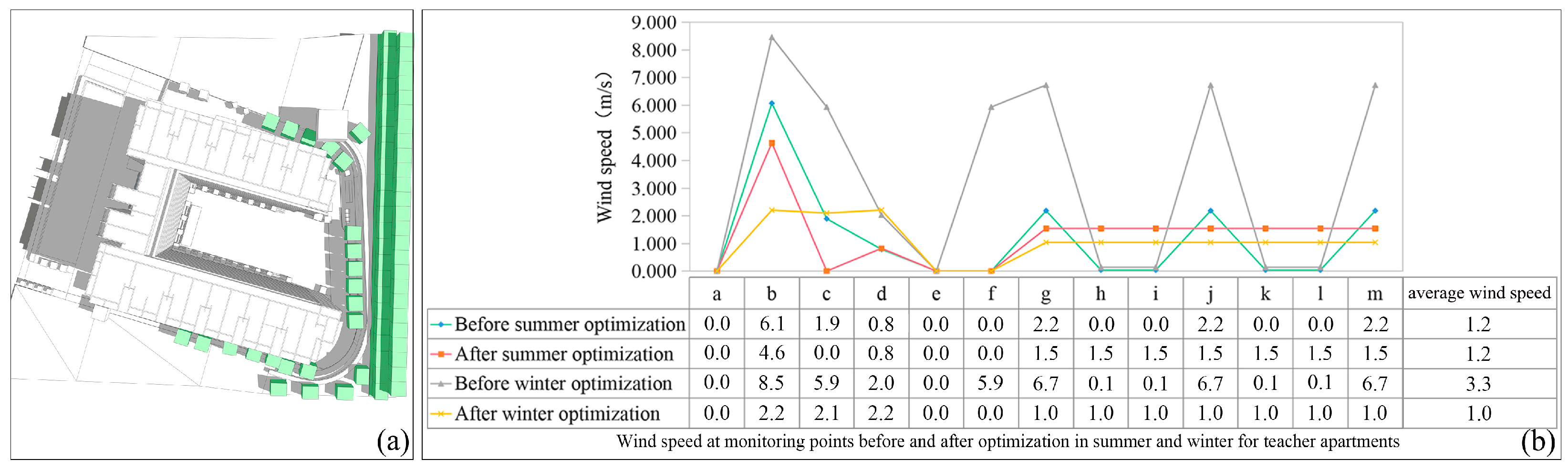
Figure 4a) and 13 points most commonly involved in crowd activities in the courtyard space (
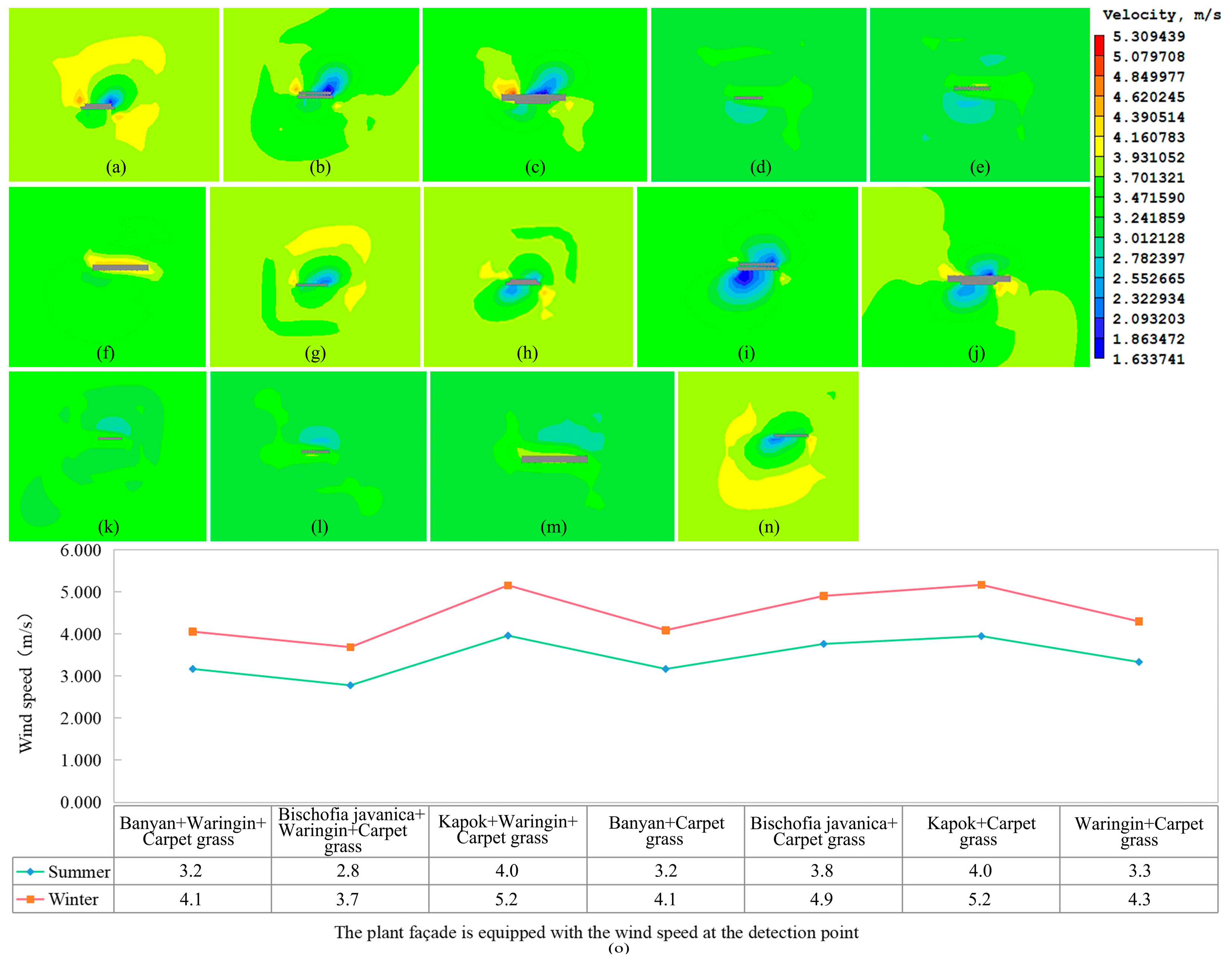
Figure 4b) were chosen; ② In terms of plant configuration, wind speed detection points were selected as the wind shadow area of plant configuration according to seasonal changes (
Figure 4c–f) to explore the wind reduction efficiency of plants.
- (2)
Onsite Experiment Method
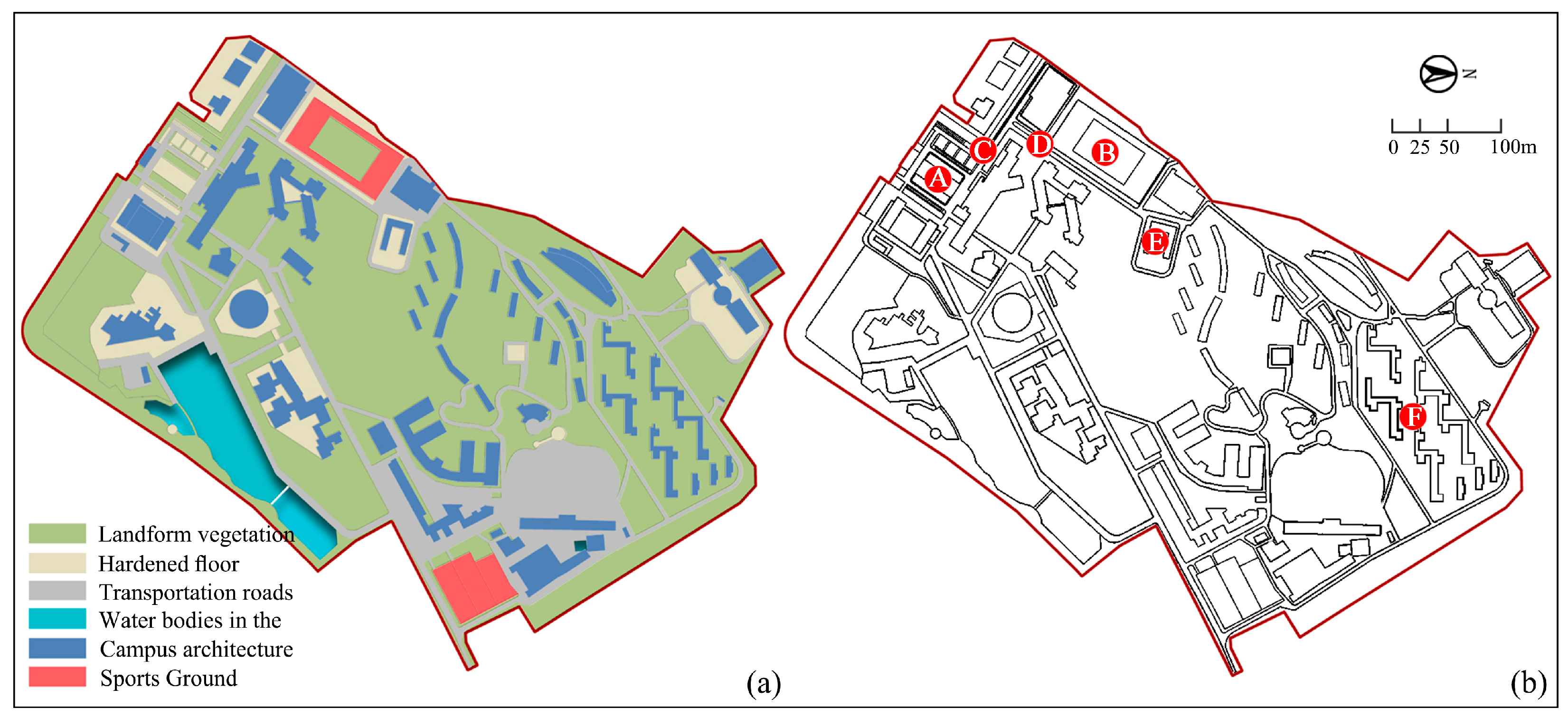
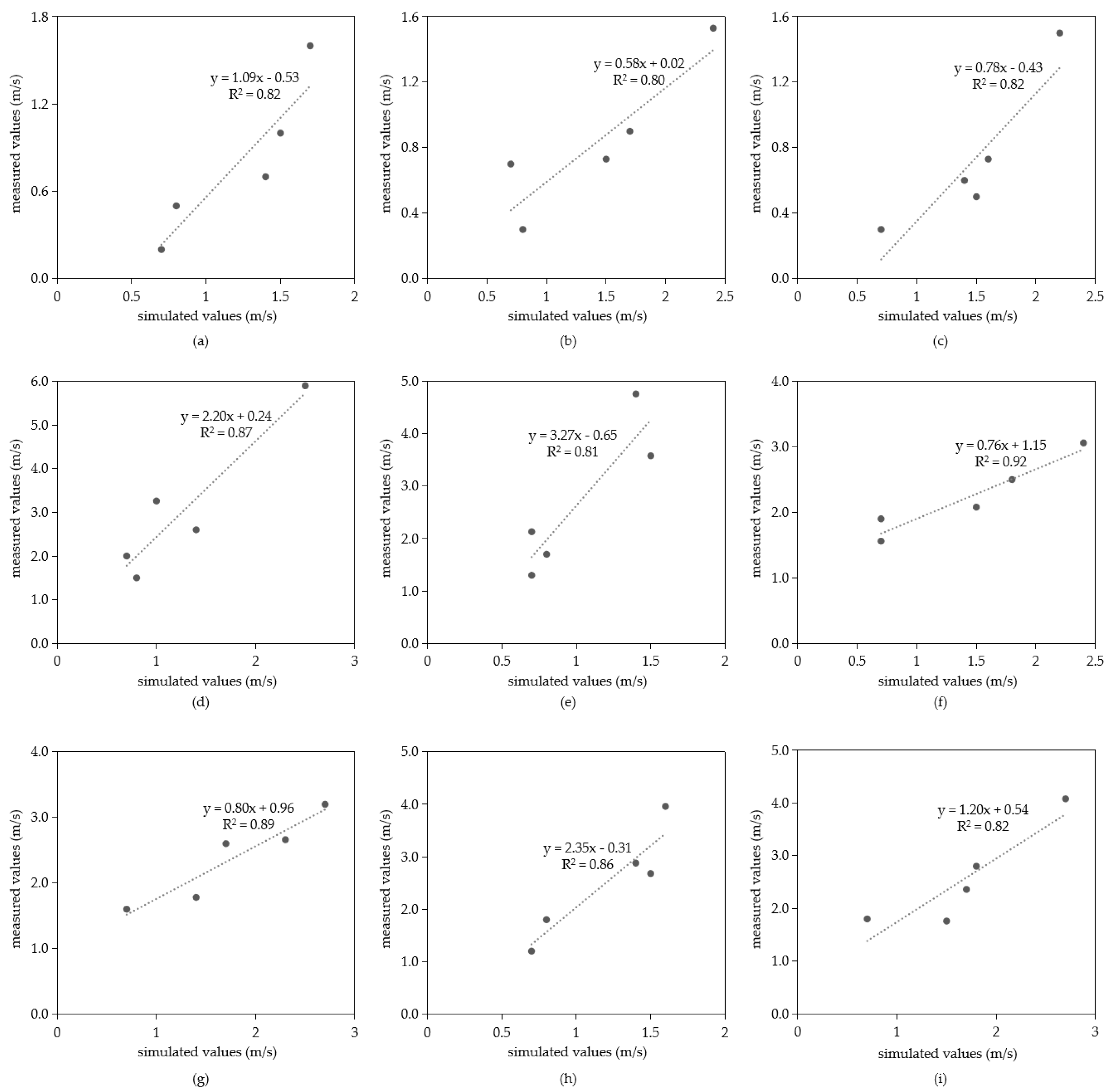
To validate the correlation between observed and modeled wind speeds, we conducted measurements of the outdoor wind conditions at the Donghai Campus of Quanzhou Normal University during sunny and partly cloudy summer days. From 9:00 a.m. to 5:00 p.m. on 30 September 2022, the NK 5500 LINK wind speed meteorological instrument was used, and multiple people were simultaneously positioned and observed to conduct fixed-point measurements in six measurement areas, identified as A, B, C, D, E, and F, on the campus. Firstly, a tripod-fixed anemometer was used for testing in each of the six measurement areas, positioning the inlet of the anemometer at a height of 1.5 m above the ground. Secondly, data was collected hourly, and the average wind speed within a one-minute timeframe of each measurement point was recorded for every data point (wind speed values were measured at minimum, average, and maximum levels every 10 s over the course of 1 min). During the hours of 9:00 a.m. to 5:00 p.m., 6 groups and 54 valid wind speed data points were obtained. Then, an evaluation was performed to compare and analyze the authentic wind conditions in different outdoor locations on campus, utilizing the measured data. The NK500LNK anemometer has a wind speed measurement standard range from 0.6 m/s to 40.0 m/s, featuring a resolution of 0.1 and an accuracy of ±3%.
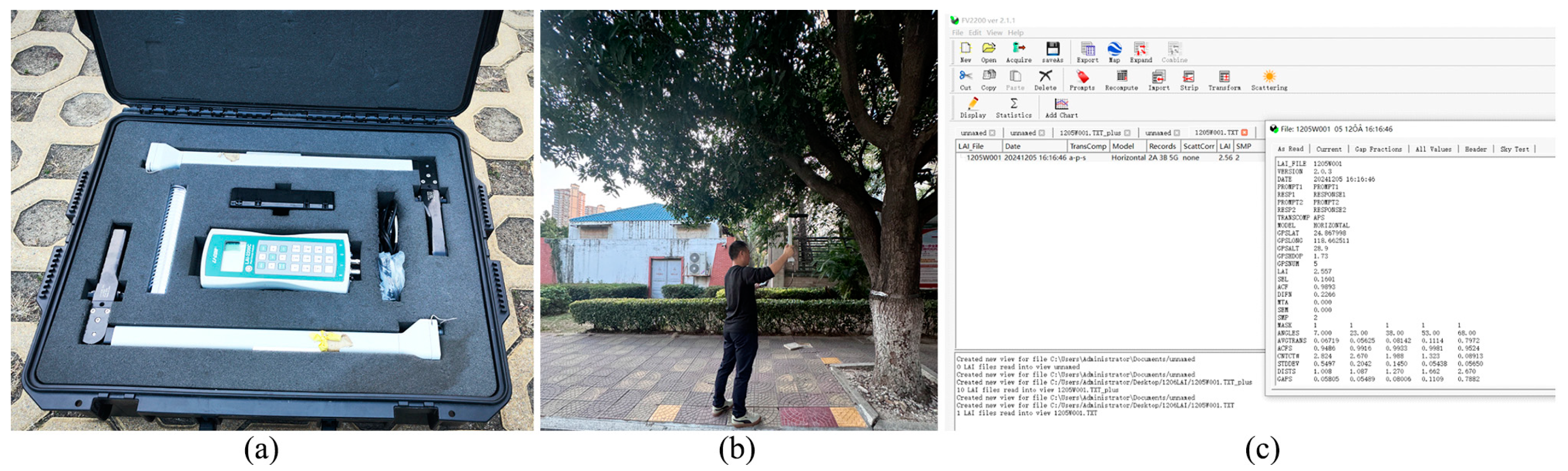
On 6 December 2024, leaf area index (LAI) measurements were conducted on typical plants in the main entrance square of the campus (
Figure 5) using the LAI-2200C Plant Canopy Analyzer (LI-COR Biosciences, Lincoln, Nebraska, USA). Measurements were taken in four directions beneath the canopy of each plant to determine the corresponding leaf area index. Subsequently, the measured data from the analyzer was transferred to a computer for analysis using the FV2200 V 2.1.1 software to derive the LAI values for each plant.
- (3)
3D Model Construction
Establishment of Plant Configuration Model: Through on-site investigation of the plants in the main entrance square, it was found that the plants are mainly divided into three categories: herbs, shrubs, and trees. Among them, the herbs include carpet grass, the shrubs include waringin and
Aglaia odorata lour, and the trees include
Erythrina indica, banyan,
Bischofia javanica, mango trees,
Chorisia speciosa, and kapok. Aerial surveys were conducted on the canopy height, width, and trunk height of various plants, and the leaf area index of different plants was measured using the LAI-2200C Plant Canopy Analyzer (
Table 1). The research by Li et al. indicates that the rectangular model has advantages such as simple modeling, fast calculation, and good convergence [
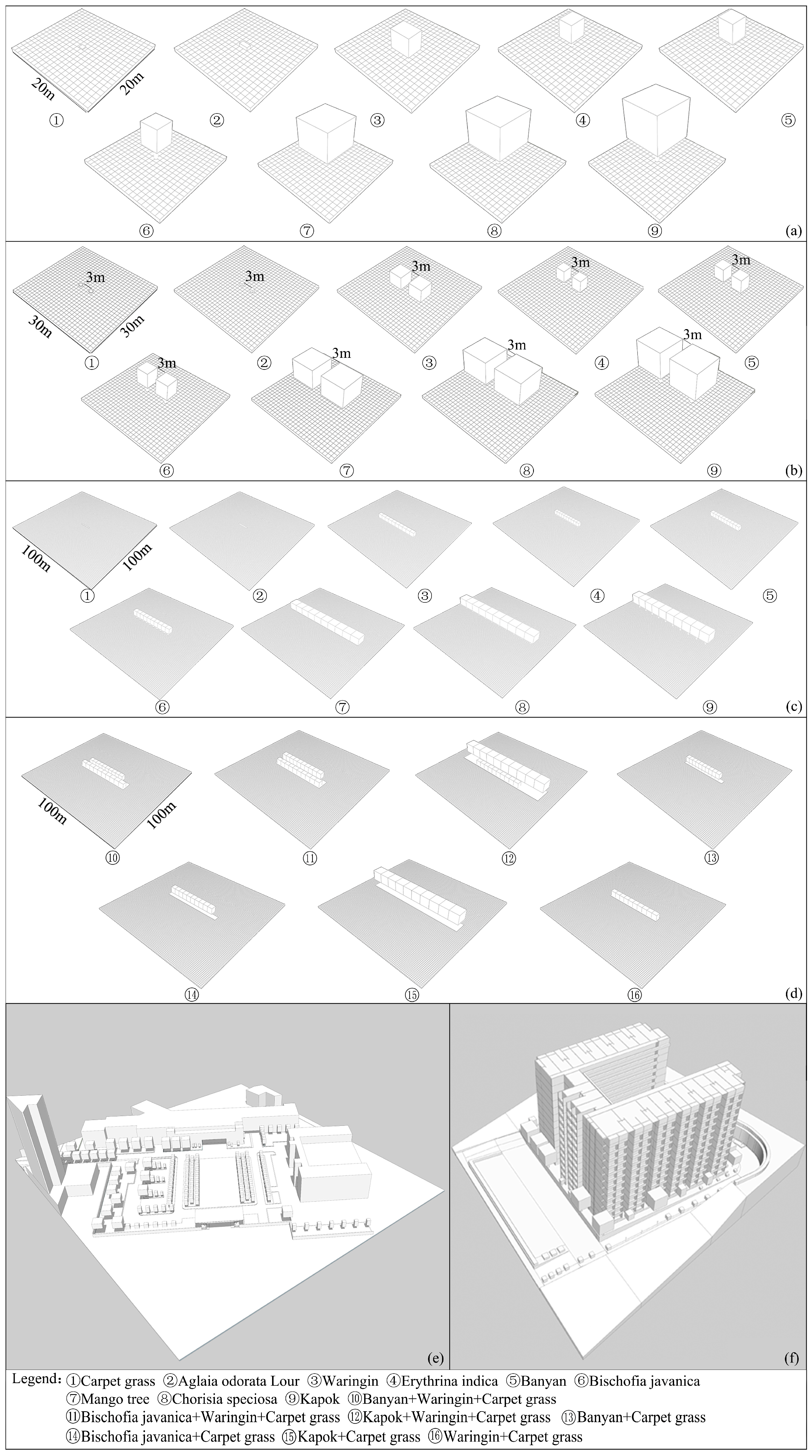
23]. Therefore, the simulation employed the technique of simplifying the rectangular model and utilized SketchUp v.2021 software to create a three-dimensional model for calculating the outdoor wind field for 34 plant configurations, categorized into planar and vertical configurations (refer to
Table 2 and
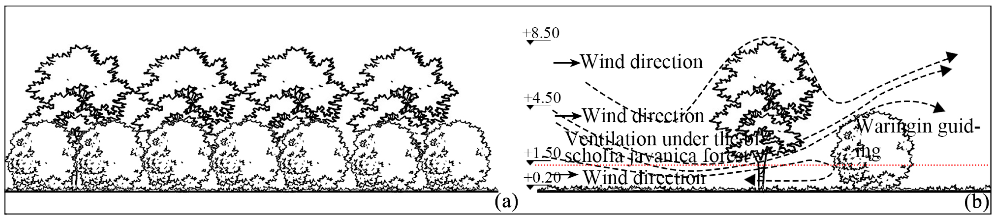
Figure 6a–d). In terms of the planar configuration, under opposite planting conditions, the crown spacing between two plants is 3 m. Under the row planting condition, it is set to single-row dense planting, with a crown spacing of 0 m, for a total of 10 trees. In terms of the facade configuration, select plants with better wind regulation efficiency when planting alone to further explore the facade configuration scheme of plants with better wind reduction efficiency. Through solitary planting experiments, it was found that the wind regulation efficiency of banyan,
Bischofia javanica, and kapok was relatively good, while that of waringin in shrubs was relatively good. Therefore, the facade configuration scheme of trees + shrubs + grass includes three types: banyan + waringin + carpet grass,
Bischofia javanica + waringin + carpet grass, and kapok + waringin + carpet grass. The facade configuration scheme of trees + grass includes three types: banyan + carpet grass,
Bischofia javanica + carpet grass, and kapok + carpet grass. The facade configuration scheme of shrubs + grass only includes one type: waringin + carpet grass.
Establishment of an outdoor space model: Using the measured CAD v.2021 topographic map of the campus, create a three-dimensional model with SketchUp v.2021 software to simulate outdoor wind flow in the main square and courtyard spaces of a single building. Make necessary simplifications and rounding of the model details without impacting the calculation results (
Table 2,
Figure 6e,f).
Change the outdoor space and plant configuration models to STL format, and then import them into PHOENICS software for simulating the wind environment. Retrieve the simulation results for the wind environment at a pedestrian height of 1.5 m (Z = 1.5 m) above ground level.
- (4)
CFD Simulation Settings
There are several software choices for carrying out CFD simulations, such as PHOENICS v.2016, ANSYS FLUENT v.2019, ENVI-met v.2021, Airpak v.2016, and Butterfly v.2018. PHOENICS, considered the original commercial software for fluid and heat transfer calculations, is increasingly favored by researchers for simulating wind conditions in different settings like residential areas, school campuses, and landscape gardens. Through the use of PHOENICS for CFD simulation, researchers have discovered that different height distribution patterns can influence alterations in both wind speed and pressure [
24]. Making changes to the architectural layout can be a useful strategy for decreasing community energy consumption and carbon emissions [
25]. The arrangement of courtyard plants has a significant effect on the outdoor microclimate, residential wind, and thermal comfort [
26]. Changes in the arrangement and proportion of architectural spaces can create efficient ecological buffer zones [
27]. ENVI-Met is primarily used for thermal comfort and has extensive experience and data backing in simulating urban microclimates. It offers precise simulation results for specific urban environments and climate conditions [
28]. PHOENICS software, in contrast to ENVI-met software 4.0, is capable of modeling intricate three-dimensional fluid dynamics, encompassing turbulence and eddies, essential for the precise evaluation of wind conditions. By employing meticulous grid segmentation and sophisticated numerical techniques, PHOENICS can deliver detailed wind parameters, such as speed and direction, thus augmenting the assessment of wind comfort. Hence, the PHOENICS software is ideal for modeling wind conditions within the square area under investigation. The setup of the CFD simulation and the creation of the model will be outlined in the following section.
Model selection: In PHOENICS, the RNG
k-
ε turbulence model is employed, utilizing Equations (1) and (2) alongside the PRESTO discrete equation and the integrated PARSOL function settings for simulating velocity–pressure coupling. Implement small-scale network configurations in the core area to enhance calculation accuracy. The automatic convergence detection feature in PHOENICS ensures that simulation results converge reasonably with an accuracy level of 10
−5 [
29].
The equations utilize the symbols k for turbulent kinetic energy and ε for turbulent dissipation rate, and are solved using the software PHOENICS v.2016.
Grid setting: The length and width of the calculation domain are five times larger than those of the corresponding scene model, and the height is three times greater than the model’s height (
Figure 7) [
30]. The calculation domain measures 5 W × 5 L × 3 H (
Table 3 shows a comparative analysis of simulation data using various computational domain heights, indicating that the height of the computational domain has no impact on simulation outcomes). The computational domain grid is divided into two regions: the center and the edge, with specific grid densities assigned to each. The grid densities are as follows: coarse meshes, X
min = Y
min = Z
min = 0.27 H; fine meshes, X
min = Y
min = Z
min = 0.13 H; and finest meshes, X
min = Y
min = Z
min = 0.06 H (
Table 4 presents a comparative analysis of simulated data using various computational domain grid densities, showing that higher grid resolutions result in improved accuracy at the cost of longer simulation durations) [
31]. Simulation accuracy is enhanced and the number of grid segments is decreased by the grid setting, which improves time efficiency. Using a fixed pressure and zero gradients, an outlet boundary condition was defined. The ground roughness parameter
α, was set to 0.2.
The inflow profile at the top boundary had a constant horizontal velocity and turbulent kinetic energy, while the left and right symmetric boundaries were considered slip walls without gradients.
By utilizing Equation (3), it is possible to calculate the gradient of the oncoming wind at the inlet:
where
u(z) is the horizontal velocity at height
z, and
u0 is the horizontal velocity at height
z0. In this model,
u0 = 3.4/3.5 m/s (summer/winter),
z0 = 108.4 m, and
α = 0.25 [
32].
The turbulent kinetic energy,
k (m
2/s
2), and its dissipation rate,
ε (m
2/s
3), are set as follows:
where
u* is the friction velocity,
δ is the depth of the boundary layer, and
K is the von Karman’s constant. In this model,
u* = 2.7/2.9 m/s (summer/winter),
K = 0.4, and
Cµ = 0.09 [
30].
Trees in the model were parameterized as a one-dimensional column, where the normalized LAI was scaled to tree height [
33]. Observing the non-uniform vertical distribution of LAI allows for easy identification of different types of vegetation, as LAI changes depending on height, influenced by crown shape, height, and canopy edges [
34]. When it comes to turbulence models, tree crowns are seen as porous media, with individual tree branches being compared to the crown [
35]. The tree canopy causes a reduction in the kinematic energy of airflow due to drag and pressure, leading to utilization of resistance in the momentum equation to model the impact of vegetation on turbulent flow patterns. The momentum equation includes a sink term to factor in turbulence resistance caused by the canopy layer as follows:
where
Cd is the drag coefficient,
is the vector speed on foliage surface (m/s), and
is the Cartesian velocity in
direction (m/s).
Additional source terms in the momentum equation can demonstrate the correlation between airflow and tree canopy turbulence as follows:
In this investigation,
βp,
βd,
C4ε, and
C5ε are empirical constants with values of 1.0, 3.0, 1.5, and 1.5, respectively.
βp denotes the average fluid kinetic energy of the wake flow,
k, produced by the drag force of the canopy; whereas
βd indicates the kinetic energy,
k, dissipated by the short circuits of Kolmogorov energy gradients [
36,
37,
38,
39].
Wind conditions setting: As per the “Design Code for Heating, Ventilation and Air Conditioning of Civil Buildings” (GB507360-2012, China), “China Weather Network”, “China Meteorological Network”, and “China Meteorological Data Network”, Quanzhou experiences an average wind speed of 4.7 m/s and an average air temperature of 27.8 °C during the summer, with a relative humidity of 85% and a mean radiant temperature of 31 °C. The prevailing wind direction is southwest. In the winter, the average wind speed increases to 6.13 m/s, while the average air temperature drops to 14.6 °C. The average relative humidity is 75% and the mean radiant temperature is 17.8 °C, with the prevailing wind direction shifting to the northeast. The seasonal dominant wind direction refers to the range of wind direction angles with the highest wind frequency within a specific season. The dominant wind direction in Quanzhou is southwest in the summer and northeast in the winter. These values are used as inflow boundary conditions for 2000 iterations.

 ,
, 


