Abstract
The use of a novel chrono-potentiometry method (abbreviated as “CP”) in the determination of the moisture content in wood (abbreviated as “MC”) above the FSP is a practical application of the electrical charging effect (or ECE). In the specific case of this CP method, the ECE consists of an electrical charging phase for the wood and a discharge phase following the interruption of the charging current. The electrical resistance, R, and the electrical chargeability, Cha(E), of three hardwood species were determined from the final potential, E1, of the charging phase and the initial potential, E2, of the discharge phase, with the three hardwood species being birch (Betula spp.), aspen (Populus spp.), and black alder (Alnus glutinosa (L.) Gaertn). An auxiliary variable in the form of U (E1; E2) was defined as a function of E1 and E2. This was used as an independent electrical variable in the calibration model for a CP moisture meter for the three tree species when it came to the moisture content (MC) region above the FSP (fibre saturation point). It was found that upon a determination of the MC in the wood, the traditional calibration model (the R-model), which uses the electrical resistance of wood, was able to predict a single-measurement precision level of +/−10% for the MC while the U-model predicted a precision level of +/−1.75% for the MC over a single MC measurement in the wood.
1. Introduction
Below the FSP, the electrical resistance of wood is a time-independent constant [1,2,3]. At moisture contents that are above the FSP, the electrical resistance of wood becomes time-dependent [4,5,6,7]. The various types of calibration functions that are available via a novel moisture meter were analysed and modelled by Tamme (2021) [8]. The theoretical background for the wood moisture meter, based on the electrical charge effect (ECE), was also presented by Tamme et al. (2022) [9]. According to the classification of measuring procedures, which has been adapted by Tamme et al. (2022) for the study of electrical properties in wood (see Table 1), it is possible to induce the ECE at a constant charge (or polarisation) voltage (or potential). Such a means of electrically charging the wood is referred to as a potentiostatic charging regime. It is also possible to use constant current charging to induce the ECE in wood. This form of charging is referred to as galvanostatic charging. The potentiostatic charging–discharging cycle and the galvanostatic charging–discharging cycle are both referred to as chrono-methods [10]. Those chrono-methods, which were used in the papers [5,8,9], are all potentiostatic, i.e., the electrical charging of the wood takes place at a constant voltage between the measuring electrodes (or potential relative to the reference electrode, RE, to use MetrOhm Autolab terminology). It would be interesting to know which results could be obtained in terms of determining the MC of wood in the MC region above the FSP by means of the electrical charging of the wood in the galvanostatic mode and what could be the corresponding calibration models in the wood moisture meter.

Table 1.
Summary of the main statistical parameters of the actual MC%, R, and Cha(E), as measured during the experiment, for the three tree species.
The aim of the present work was to use chrono-potentiometry (CP) in tandem with the galvanostatic charging mode as one possible method to determine the MC of wood and the chargeability of wood (Cha(E)) in the MC region above the FSP and to develop relevant calibration models.
2. Materials and Methods
2.1. Materials
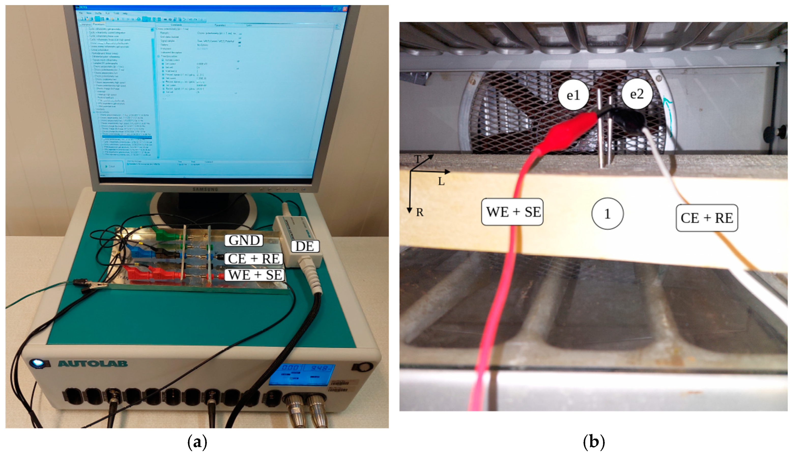
Calibration models were constructed for three hardwood species: birch (Betula spp.), aspen (Populus spp.), and black alder (Alnus glutinosa (L.) Gaertn). For the determination of the MCs in the wood, test specimens were used for those species, which formed part of this study, with dimensions of 500 mm (length in the longitudinal direction), 150 mm (width in the tangential direction), and 36 mm (thickness in the radial direction). The following drying method was used to vary the average MC in the wood: Test specimen 1 was dried out in a climatic chamber [11] (see the photo in Figure 1b). The longitudinal (L-direction in Figure 1b) ends of the test specimen (a 150 mm × 36 mm cross-section of a twig-free board) were carefully moisture-insulated with a double layer of nitrocellulose lacquer and a single layer of aluminium tape. The tangential (T-direction in Figure 1b) sides of the board were insulated against moisture transfer with just a triple layer of nitrocellulose lacquer [12]. Due to this longitudinal and tangential moisture insulation, the drying moisture could only exit the wood in the radial direction from both sides of board 1. The result was that during the drying process, the test specimen acquired a one-dimensional (1-D) moisture profile (i.e., MC distribution), symmetrical in respect to the board’s central area. Detailed data on the drying schedule that was used in the drying experiment and on the radial moisture profiles at different depths, which result from the drying of different hardwood species, can be found in Tamme et al. (2023) [13]. The recording of electrical quantities was based on the requirements of EN 13183-2:2005 [14] for the insertion of measuring electrodes into wood, the spacing of the measuring electrodes, and the measuring depth. According to EN 13183-2:2005, measuring electrodes (preferably insulated pin electrodes that are made of stainless steel) [15] are to be inserted into the wood in a radial direction, with a spacing of 30 mm and to a depth of one-third of the thickness of the board when measured from the board’s surface. The electrical field between the electrodes is then directed in a tangential direction, perpendicular to the longitudinal direction (see the photo in Figure 1b). The standard EN 13183-2:2005 assumes that at a measurement depth of one-third of the board thickness, the local MC in the wood is approximately equal to the board’s average moisture content, something that is easily determined by weighing it (see Table 1), as stated in the standard ISO 3130:1975 [16]. The numerical equivalence of the local MC as measured at a depth of one-third of the board thickness, along with the average board MC, is mathematically verifiable in the MC region below the FSP [17]. Above the FSP, the occurrence of a numerical equivalence between the local MC and the average MC probably depends upon the drying plan being used and on the board’s thickness. Therefore, the implementation of the one-third table depth requirement of the standard EN 13183-2:2005 would necessitate at least one experimental confirmation of the approximate numerical equivalence of the average MC, both in the test specimen and in the local MC, measured at a one-third board depth. In Figure 2a, the relevant experimental confirmation is illustrated using alder as an example adapted from the article by Tamme, 2023 [13].
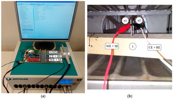
Figure 1.
(a) MetrOhm Autolab with self-made junction box. (CE + RE) and (WE + SE)—signal cables, DE—differential electrometer, GND—ground. (b) Test specimen 1 in climate chamber [11]. e1 and e2—pin electrodes; L, T, and R—anatomical directions of the wood.
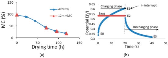
Figure 2.
(a) The example of the approximate equality of the average moisture content of the specimen and the local moisture content measured at the depth of 1/3 of the surface of the test specimen (adapted from [13]). (b) The CP general shape of the charge–discharge cycle in the example of the birch wood.
2.2. Methods
After the measuring electrodes were inserted into the wood in accordance with the EN 13183-2:2005 standard, those electrical quantities that are required for the calibration model were then measured. In one test piece at a randomly selected electrode insertion position, placed inside a climatic chamber along with the electrodes and a signal cable, one measurement of the charge–discharge cycle was carried out by means of the CP measurement procedure (see Figure 1a,b and Figure 2b and Table 1). A two-electrode measuring mode was used in which the coupling electrode (CE) and the reference electrode (RE) were coupled together, i.e., one symmetrical measuring electrode was formed based on (RE+CE). In addition, the working electrode (WE) and the sensitive electrode (SE) were coupled together, i.e., a second symmetrical measuring electrode was formed based on (WE+SE). Following the completion of the measurement of the CP cycle, the test specimen was removed from the climatic chamber before being weighed, and the electrodes were removed to be inserted into the next randomly chosen location on the test specimen. The time required to weigh the test piece and change the electrode positions was approximately one minute. Test specimen 1 was then placed back into the climatic chamber with the measuring electrodes in the new position (see the photo in Figure 1b). Then, after waiting for about one minute for the temperature and humidity in the test specimen’s surface layer to equalise once more with the environment within the climatic chamber, the next CP cycle was measured (see Figure 2b), then the next cycle was measured, and so on. In total, approximately twenty to thirty replicate measurements were carried out at various random locations for the measuring electrodes on test specimen 1, at one average MC level for the test specimen but always to a depth of 1/3 of the surface of the board. The typical shape of one CP cycle, as resulted from the measurements, is shown in Figure 2b. From point E0 to point E1, the wood is electrically charged at a constant current of I = 1µA, as previously set out on the measurement procedure’s CP sheet. The charging curve from E0 to E1 consists of two hundred data points, and the charging phase lasts for twenty seconds. Under these conditions, it was guaranteed that an electrical charge, which would be equal to twenty microcoulombs, would pass through the space between the electrodes during each repeated measurement. The average value for the potential Eavg in the charging curve is represented by a horizontal series of points that are parallel to the time axis. At point E1, there is an interruption in the charging current, and the potential drops over a measuring interval of 0.1 s to point E2. This abrupt drop (E1 to E2) is called the “Ohmic drop”. It is used to determine the electrical resistance of the wood (MetrOhm Autolab, 2024) [18]. The curve that is formed by the data points between points E2 and E3 is referred to as the “discharging curve”. This also has a time duration of twenty seconds, and it consists of two hundred data points. Thanks to the CP cycle, it was possible to calculate the electrical resistance, “R’”, of the wood, along with the wood’s electrical chargeability, Cha(E), and its average electrical resistance, Ravg.
The Ohmic drop is expressed through MetrOhm Autolab (2024) [18] as follows:
where E1 − E2 is the Ohmic drop, from which R is expressed through Ohm’s law as
When using the definition of electrical capacitance, the wood’s electrical capacitance at potential E1 was determined as follows:
where C is the electrical capacitance of the wood at the end of the charging phase at the twentieth second of charging and I = 1 µA = const at each charging phase and for any wood species.
Chargeability [9] was determined through the equation
where Cha(E) is the electrical chargeability of the wood according to the potential jump before and after the current cut-off.
The average electrical resistance of the wood in terms of mega-ohms was found via Ohm’s law:
The average electrical capacitance of the wood in microfarads was determined from Equation (3) as
where
2.3. A Quality Assessment for the Wood Moisture Meter’s Calibration Model
The quality of the calibration model was assessed theoretically as a regression model that was adapted to the calibration task [19,20]. The standard error margin (or “SE”) was expressed for the model, or a numerically close RMSE was used, along with the model’s p-value: regression residuals were subjected to various tests (Q-Q plot, histogram, Kolmogorov–Smirnov test, and Shapiro–Wilk test) [21]. From the point of view of practical metrology [21,22], the most important information for any user of the moisture meter is the model’s estimation of the precision of an individual measurement under repeatable conditions. This precision estimation may in turn depend upon the average MC in the wood within the region above the FSP value [22]. Rozema (2010) [23] presented a classification for the assessment of the quality of calibration models for resistive-type wood moisture meters. Tamme et al. (2021) [24] showed the lowest-quality class being selected from Rozema’s classification and being named as Rozema’s criterion (Rcr). Rcr was defined as a constant numerical value of the single MC% measurement’s tolerance interval, with a 95% confidence level that must be met in the MC region above the FSP value for any average MC value of wood (Rcr < 3.5% MC). Tamme [24] has shown (2021) that Rcr may be difficult to achieve for various wood moisture meters in the region above the FSP. As an alternative, something was proposed that was referred to as a multiple model, wherein the arithmetic average of 16 MC measurements play out the role of a single measurement. An example of a practical realisation of the multiple model is the use of sixteen parallel MC measurement channels in a kiln, with an average of the readings being taken at each measurement interval (e.g., each hour).
3. Results
3.1. Average Charging Number, Cha(N)avg, in the Wood
A function was written that was based on Equations (5) and (6):
Equation (7) is valid for the average MC above the FSP in any wood type.
And after the logarithmic of function (7), it was found that
Equation (8) is illustrated by Figure 3.
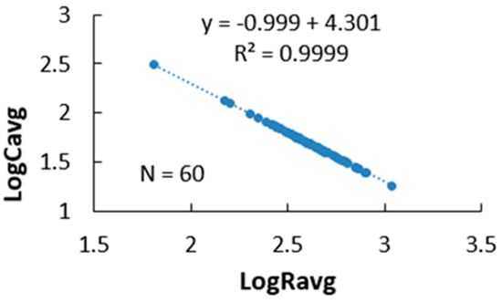
Figure 3.
The average electrical charging number for birch wood under galvanostatic charging at any average MC value of the wood.
In Figure 3, the logarithmic average electrical resistance, Ravg, is shown in kilo-ohms and the logarithmic average electrical capacitance is shown in microfarads, with the number of observations at n = 60 for the CP-cycle charging phase. When processing the experimental data, it was found that the average charging number, Cha(N)avg, in wood does not depend upon the wood’s moisture content.
3.2. Selecting Measurement Data for the Moisture Meter’s Calibration Model
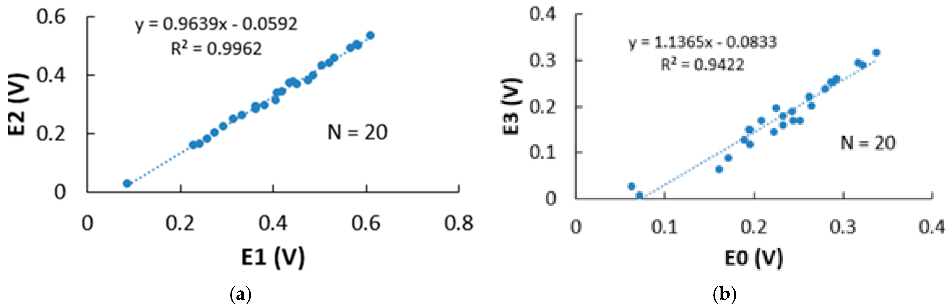
The measurement data consisted of a non-electrical quantity—i.e., the MC measurement data for the actual (gravimetric) moisture content of the wood and the charging–discharging cycle as recorded by the CP measurement procedure. The measurement points were clearly numerically asymmetric (Tamme, H, 2023) [25]. One measurement from the actual MC % corresponded to four hundred data points of electrical potential as obtained by the CP measurement procedure. Clearly, the number of data points for the electrical measurements needed to be drastically reduced. Initially, four characteristic points were selected for the charge–discharge cycle, E0, E1, E2, and E3, and also the average potential, Eavg, during the charge phase (see Figure 2b). The strengths of the linear correlations between E1 and E2 and between E0 and E3 were then investigated. The results are shown in Figure 4a,b. There is a strikingly strong correlation between E1 and E2 (R2 = 0.998). Thanks to this, the characteristic points E0, E3, and Eavg were dropped from the calibration model, with it now using only E1 and E2 as electrical variables. Tamme et al. (2021) [8] has shown that if two electrical quantities are strongly correlated and their random deviations are in the opposite phase with respect to the average value, then it is possible to make the random deviations converge into a single point by defining an expedient auxiliary variable. This characteristic point was referred to as the model’s focal point.
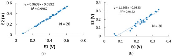
Figure 4.
(a) A plot of the linear correlation for parameters E1 and E2. (b) A plot of the linear correlation for parameters E0 and E3.
In this paper, the auxiliary variable, U, is defined as follows:
where U is the auxiliary variable, E1 and E2 are the potentials as measured at the actual average moisture content level, and k is a constant that was found through machine learning. Therefore, it is possible to use the characteristic points E1 and E2 to find the wood’s electrical resistance levels; to find the electrical chargeability levels; and to define an auxiliary variable, U, for the construction of focusing the calibration models.
3.3. Calibration Models for Different Tree Species and a Determination of Electrical Chargeability, Cha(E), for Different Tree Species in Terms of the Galvanostatic Charging Mode
Figure 5a,b illustrate the raw data obtained from the experiment for the wood electrical charging phase and the wood discharging phase. It was found that a logarithmic trend line was well-suited to be able to approximate all charging and discharging curves.
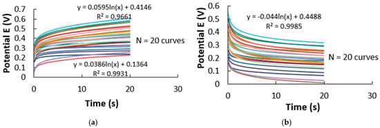
Figure 5.
(a) An example of a cloud of experimentally determined potential curves for birch wood during the electrical charging phase. (b) An example of a cloud of experimentally determined potential curves for birch wood during the electrical discharge phase.
Clarification: the SE interval, i.e., the “narrow interval”, is not shown in Figure 6, Figure 7, Figure 8 and Figure 9 for the calibration models, but its value is given in Table 2.
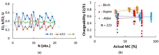
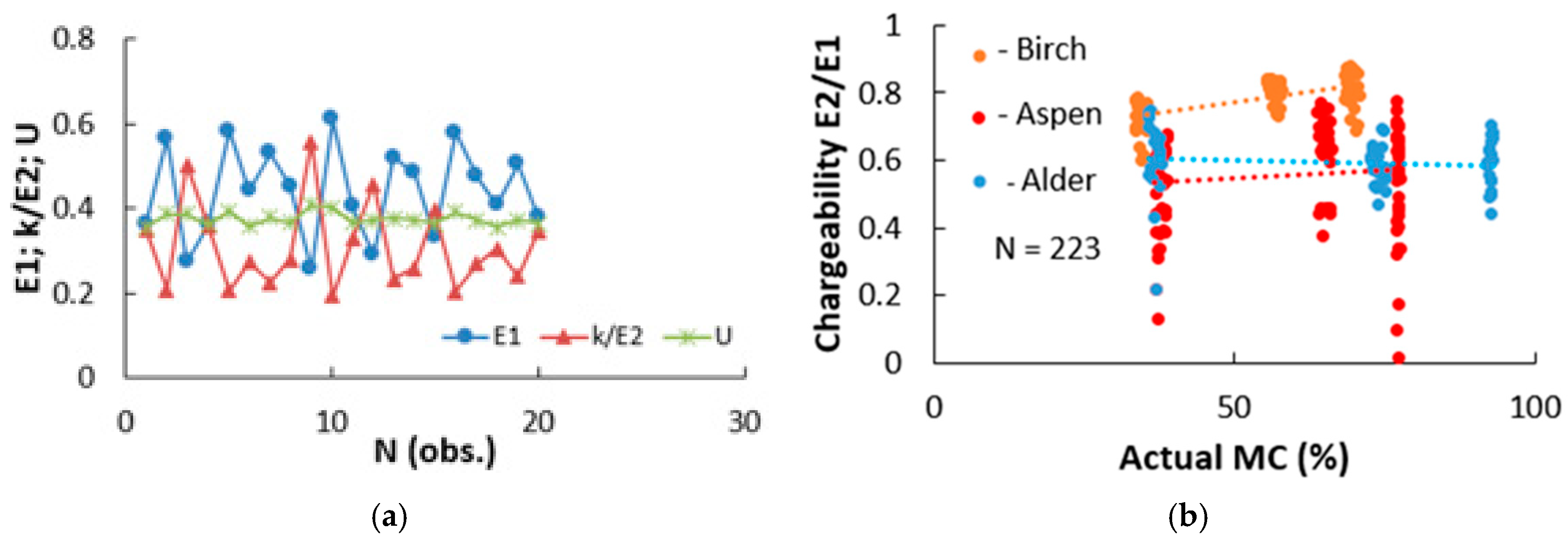
Figure 6.
(a) An example of a minimisation mechanism for random measurement errors in measured electrical quantities in connection with a birch test specimen during the composition of the auxiliary variable, U, using Equation (9) to define the auxiliary variable. (b) The dependence of electrical chargeability on the wood’s MC in the region above the FSP, as calculated using Equation (4) for three tree species.
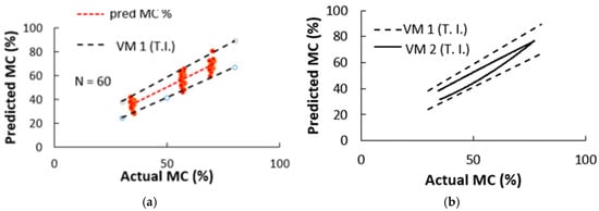
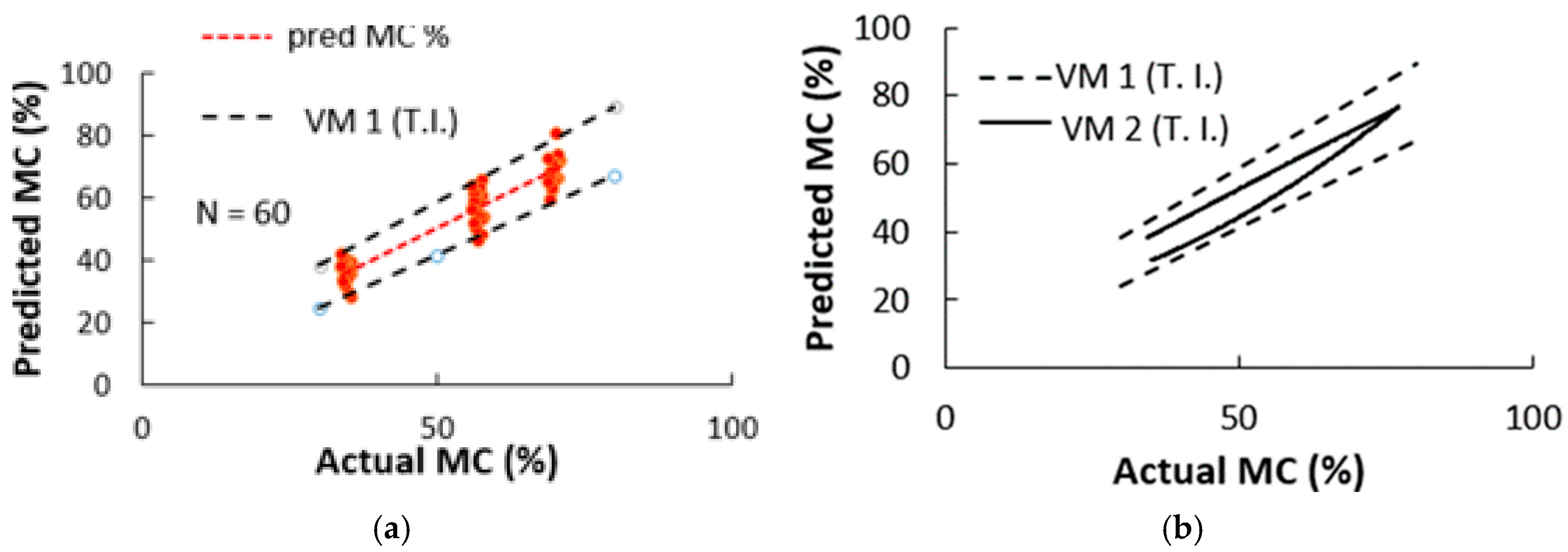
Figure 7.
(a) The dependence of the MC on the actual (gravimetric) MC for birch wood, as predicted in the R-model of electrical resistance. (b) The dependence of the MC as predicted from the U-model for birch wood focussing on the actual MC. To be able to create a comparison, the tolerance interval for the focussed model is supplemented by the tolerance interval from the previous, Figure 6a (the R-model), i.e., the “wide interval”.
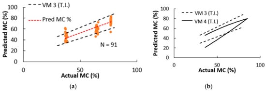
Figure 8.
(a) The dependence of the MC on the actual (gravimetric) MC for aspen wood as predicted in the R-model of electrical resistance. (b) The dependence of the MC as predicted in the U-model for aspen wood focussing on the actual MC. To be able to create a comparison, the tolerance interval for the focussed model is supplemented by the tolerance interval from the previous, Figure 6a (the R-model), i.e., the “wide interval”.

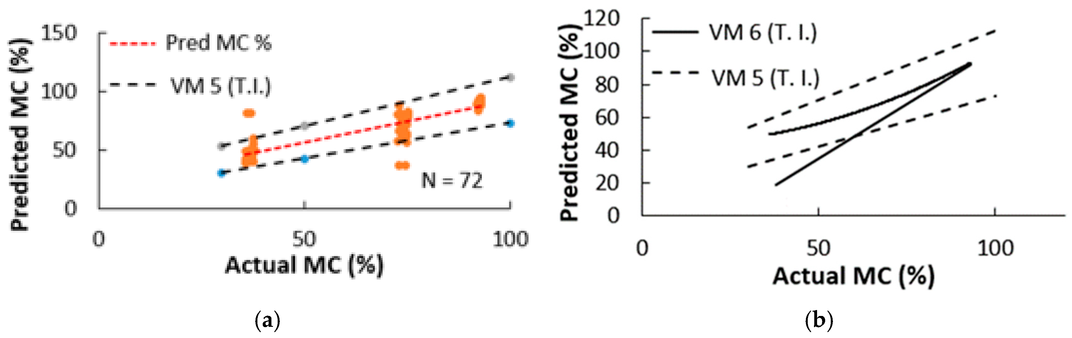
Figure 9.
(a) The dependence of the MC on the actual (gravimetric) MC for alder wood as predicted in the R-model of electrical resistance. (b) The dependence of the MC as predicted in the U-model for alder wood focussing on the actual MC. To be able to create a comparison, the tolerance interval for the focussing model is supplemented by the tolerance interval from the previous, Figure 6a (the R-model), i.e., the “wide interval”.
Table 2.
Significant statistical characteristics of validation models (VMs) for three hardwood species—birch (Betula spp.), aspen (Populus spp.), and black alder (Alnus glutinosa (L.) Gaertn.)—under repeatability conditions and at wood MCs above FSP.
Explanation of the legends of Figure 7, Figure 8 and Figure 9: “T.I.”, that is, the “wide range”, is the range where 95% of all individual measurements in the sample lie. “VM” literally means the reference model (RM) [8]. The validation model (VM) compares the actual MC% values under repeatability conditions with the values calculated based on the calibration function.
Table 2 shows the results that came from the quality assessment of the calibration model under repeatable conditions for the three tree species [20,21,22].
4. Discussion
- For three hardwood species—birch (Betula spp.), aspen (Populus spp.), and black alder (Alnus glutinosa (L.) Gaertn)—rather surprisingly, it was found that the average electrical chargeability, Cha(E), in the wood was practically independent of the wood’s average MC in the region above the FSP (see Table 1 and Figure 6b). The actual density of the birch wood sample was 0.66 g/cm3. The actual density of the aspen wood was 0.53 g/cm3. The actual density of the alder wood sample was 0.46 g/cm3. On the other hand, the average electrical chargeability was found to be of the same order of magnitude as the basic density (i.e., the dry weight divided by the wet volume (above the FSP)) for the same wood species. If the hypothesis of an approximate numerical equivalence between the wood’s basic density and its average electrical chargeability is confirmed by further studies, then the possibility opens up that the wood’s chargeability can be used to predict the wood’s basic density in a non-destructive way, something that is similar to that of the use of a resistograph [26].
- For three hardwood species—birch (Betula spp.), aspen (Populus spp.), and black alder (Alnus glutinosa (L.) Gaertn)—it was found that the electrical resistance, R, of the wood as determined by the CP method was suitable for the prediction of the wood’s average MC using the R-model (see Figure 7a, Figure 8a and Figure 9a and Table 2).
- For the three hardwood species, it was found that the CP-determined auxiliary variable U (E1;E2) (see Equation (9)) was suitable for predicting the average wood MC using the U-model, with a prediction accuracy about five times better than the one that involved the R-model (see Figure 7b, Figure 8b and Figure 9b and Table 2).
- Comparing the tolerance intervals (T.I.s) of the R-model (VM 1, VM 3, VM 5) and U-model (VM 2, VM4, VM6) single measurements shown in Figure 7b, Figure 8b and Figure 9b, similar trends as in the paper by Tamme (2021) [8] were observed. Namely, the T.I. of the R-model expanded with increasing wood MC, while the T.I. of the U-model concentrated at a single point with increasing wood MC.
- Table 2 shows that the standard error (SE) of the U-model is smaller than the SE of the R-model for all three tree species modelled in this paper.
- When comparing the RMSE of the validation model of the NIR method [27] and the SE of the validation model of the CP method, the RMSE of the NIR method was between 11.29 and 11.38 MC%, depending on the used model. This is of the same order of magnitude as the SE of the R-model of the CP method (see Table 2). We note here that the RMSE and SE are numerically very close quantities because their definition formulas differ only by one degree of freedom. If we compare the RMSE of the validation model of the microwave method [28] and the SE of the validation model of the CP method, the microwave method has an RMSE = 1.9 MC%. However, the CP method (U-model) validation model has an SE = 1.95 MC % (see Table 2). Thus, the RMSEs (SEs) of the microwave and CP methods were practically equal. Unfortunately, in the articles on the NIR method [27] and the microwave method [28], there are no comparative data on the single-measurement tolerance interval (T.I.) of practical interest.
- For the calibration models, repeat measurements were carried out on the CP cycles under the typical indoor conditions of a kiln [13], but when it came to the CP measurement procedure, this fact had no effect on reliability (e.g., faulty measurements, random measurement noise, etc). Consequently, the CP measurement procedure can be used in practice as a possible method for the MC monitoring of wood in a kiln.
5. Conclusions
In this article, the prospective value of using the CP measurement procedure as a method for monitoring wood drying has been thoroughly experimentally researched and modelled. It was found that for the possible monitoring of wood drying using the CP method, the accuracy of a single measurement, when modelled with the U-model, is about five times better than the accuracy of a single measurement that has been modelled by using the R-model. In addition, an investigation was conducted to determine the electrical chargeability of the wood in the MC region above the FSP for the three tree species in question. It was found that the Cha(E) reading in the region above the FSP was practically independent of the wood’s MC levels, but this may correlate to the basic density of the wood. The novel CP method for the determination of the MC in wood that is being presented in this paper may be of practical use as a method for monitoring wood drying.
Author Contributions
Conceptualisation, V.T. and H.T.; methodology, V.T. and H.T.; validation, V.T. and H.T.; formal analysis, V.T. and H.T.; investigation, V.T. and H.T.; resources, V.T.; data curation, V.T. and H.T.; writing—original draft preparation, V.T. and H.T.; writing—review and editing, P.M. and A.K.; supervision, A.K. All authors have read and agreed to the published version of the manuscript.
Funding
This work was supported by the Environmental Investment Centre of Estonia (Grant No. T220055MIMP (RE.4.08.22-0049)).
Data Availability Statement
Data are contained within the article.
Conflicts of Interest
On behalf of all authors, the corresponding author states that there are no conflicts of interest.
References
- Brischke, C.; Rapp, A.O. Influence of wood moisture content and wood temperature on fungal decay in the field: Observations in different micro-climates. Wood Sci. Technol. 2008, 42, 663–677. [Google Scholar] [CrossRef]
- Brookhuis Micro-Electronics BV. Moisture Measuring Manual; Version 1.4; Brookhuis Micro-Electronics BV: Almelo, The Netherlands, 2009; p. 27. [Google Scholar]
- Uwizeyimana, P.; Perrin, M.; Eyma, F. Moisture monitoring in glulam timber structures with embedded resistive sensors: Study of influence parameters. Wood Sci. Technol. 2020, 54, 1463–1478. [Google Scholar] [CrossRef]
- Skaar, C. Some factors involved in the electrical determination of moisture gradients in wood. For. Prod. J. 1964, 14, 239–243. [Google Scholar]
- Tamme, V.; Muiste, P.; Kask, R.; Tamme, H. Experimental study of electrode effects of resistance type electrodes for monitoring wood drying process above fiber saturation point. For. Stud. 2012, 56, 42–55. [Google Scholar]
- Berga, S.C.; Gil, R.G.; Anton, A.E.; Muñoz, A.R. Novel Wood Resistance Measurement Method Reducing the Initial Transient Instabilities Arising in DC Methods Due to Polarization Effects. Electronics 2019, 8, 1253. [Google Scholar] [CrossRef]
- Suarez, S.; Sandhacker, M.; Logar, L.; Riegler, M.; Arminger, B.; Konnerth, J.; Kindl-Altmutter, W.; Tran, A. Non-invasive method to measure bulk electrical resistivity of spruce wood—Influence of moisture content and anatomical direction. Wood Mater. Sci. Eng. 2024. [Google Scholar] [CrossRef]
- Tamme, V.; Tamme, H.; Miidla, P.; Muiste, P. Novel polarization-type moisture meter for determining moisture content of wood above fibre saturation point. Eur. J. Wood Wood Prod. 2021, 79, 1577–1587. [Google Scholar] [CrossRef]
- Tamme, V.; Jänes, A.; Romann, T.; Tamme, H.; Muiste, P.; Kangur, A. Investigation and modeling of the electrical charging effect in birch wood above the fiber saturation point (FSP). For. Stud. 2022, 77, 21–37. [Google Scholar] [CrossRef]
- Eco Chemie, Metrohm Autolab B.V. Available online: https://www.metrohm.com/en/applications/ (accessed on 23 January 2025).
- Feutron Klimasimulation GmbH. Available online: https://www.feutron.de/en/weathering-chamber/ (accessed on 22 January 2025).
- Nitrocellulose Laquer. Available online: https://www.madinter.com/en/nitorlackr-nitrocellulose-lacquer-vintage-clear-gloss-spray.html (accessed on 22 January 2025).
- Tamme, H.; Kask, R.; Muiste, P.; Tamme, V. An experimental determination of the critical diffusion coefficient and critical relative humidity (RH) of drying air when optimizing the drying of three hardwood species (Birch, Aspen, and Black Alder). For. Stud. 2023, 79, 3–20. [Google Scholar] [CrossRef]
- EN 13183-2:2005; Moisture Content of a Piece of Sawn Timber—Part 2: Estimation by Electrical Resistance Method. iTeh Standards: San Francisco, CA, USA, 2005; p. 6.
- Gann Mess-u Regeltechnik GmbH. Available online: http://www.gann.de (accessed on 22 January 2025).
- ISO 3130:1975; Wood—Determination of Moisture Content for Physical and Mechanical Tests. International Organization for Standardization: Geneva, Switzerland, 1975; p. 2.
- Kretchetov, I.V. Kiln Drying; Wood Industry: Moscow, Russia, 1972; p. 440. (In Russian) [Google Scholar]
- Eco Chemie. Metrohm Autolab B.V. Available online: https://www.metrohm.com/en_nl/products/electrochemistry/modular-line.html (accessed on 24 January 2025).
- ISO 3534-1:1993; Statistics—Vocabulary and Symbols—Part 1: Propability and General Statistical Terms. International Organization of Standartization: Geneva, Switzerland, 1993; p. 46.
- R-Projekt. The R Project for Statistical Computing. Available online: http://www.r-project.org (accessed on 24 January 2025).
- ISO/IEC GUIDE 98-3:2008(E); Uncertainty of Measurement—Part 3: Guide to the Expression of Uncertainty in Measurement (GUM:1995). International Organisation for Standardization: Geneva, Switzerland, 2008; p. 120.
- Laaneots, R.; Mathiesen, O. An Introduction to Metrology; TUT Press: Tallinn, Estonia, 2006; p. 271. [Google Scholar]
- Rozema, P. Dos and Don’ts in Respect to Moisture Measurement. The Future of Quality Control for Wood & Wood Products. In Proceedings of the Final Conference of COST Action E 53, Edinburgh, UK, 4–7 May 2010; p. 9. [Google Scholar]
- Tamme, H.; Kask, R.; Muiste, P.; Tamme, V. Comparative testing of two alternating current methods for determining wood moisture content in kiln conditions. For. Stud. 2021, 74, 72–87. [Google Scholar] [CrossRef]
- Tamme, H. Development of Control and Optimization Methods for Wood Drying. Ph.D. Thesis, Estonian University of Life Sciences, Tartu, Estonia, 2023; p. 181. [Google Scholar]
- Gendvilas, V.; Downes, G.M.; Lausberg, M.; Harrington, J.-J.; Lee, D.J. Predicting Wood Density Using Resistance Drilling: The Effect of Varying Feed Speed and RPM. Forests 2024, 15, 579. [Google Scholar] [CrossRef]
- Amaral, E.A.; Baliza, L.F.; dos Santos, L.M.; Shashiki, A.T.; Trugilho, P.F.; Hein, P.R.G. Hydromechanical behavior of wood during drying studied by NIR spectroscopy and image analysis. Holzforschung 2023, 77, 618–628. [Google Scholar] [CrossRef]
- Afif, O.; Franceschelli, L.; Iaccheri, E.; Trovarello, S.; Di Florio DiRenzo, A.; Ragni, L.; Costanzo, A.; Tartagni, M. A Versatile, Machine-Learning-Enhanced RFSpectral Sensor for Developing aTrunk Hydration Monitoring System in Smart Agriculture. Sensors 2024, 24, 6199. [Google Scholar] [CrossRef] [PubMed]


Disclaimer/Publisher’s Note: The statements, opinions and data contained in all publications are solely those of the individual author(s) and contributor(s) and not of MDPI and/or the editor(s). MDPI and/or the editor(s) disclaim responsibility for any injury to people or property resulting from any ideas, methods, instructions or products referred to in the content. |
© 2025 by the authors. Licensee MDPI, Basel, Switzerland. This article is an open access article distributed under the terms and conditions of the Creative Commons Attribution (CC BY) license (https://creativecommons.org/licenses/by/4.0/).